Relative Radiometric Normalization and Atmospheric Correction of a SPOT 5 Time Series

Abstract

Multi-temporal images acquired at high spatial and temporal resolution are an important tool for detecting change and analyzing trends, especially in agricultural applications. However, to insure a reliable use of this kind of data, a rigorous radiometric normalization step is required. Normalization can be addressed by performing an atmospheric correction of each image in the time series. The main problem is the difficulty of obtaining an atmospheric characterization at a given acquisition date. In this paper, we investigate whether relative radiometric normalization can substitute for atmospheric correction. We develop an automatic method for relative radiometric normalization based on calculating linear regressions between unnormalized and reference images. Regressions are obtained using the reflectances of automatically selected invariant targets. We compare this method with an atmospheric correction method that uses the 6S model. The performances of both methods are compared using 18 images from of a SPOT 5 time series acquired over Reunion Island. Results obtained for a set of manually selected invariant targets show excellent agreement between the two methods in all spectral bands: values of the coefficient of determination (r² exceed 0.960, and bias magnitude values are less than 2.65. There is also a strong correlation between normalized NDVI values of sugarcane fields (r² = 0.959). Despite a relative error of 12.66% between values, very comparable NDVI patterns are observed.

1. Introduction

Time series of remotely sensed imagery acquired at high spatial and temporal resolution provide a potentially ideal source for detecting change and analyzing trends [1-3]. The dynamics of the radiometric signals and the vegetation indices are particularly interesting for crop monitoring, especially for mapping cropping operations (sowing, harvest, irrigation, etc.), for detecting growth anomalies, and for predicting yield.

Since multi-temporal images are often acquired by different sensors under variable atmospheric conditions, solar illumination and view angles, radiometric normalization is required to remove radiometric distortions and make the images comparable. Effects of artifacts, surface directionality and atmosphere can be corrected in an absolute or a relative way.

Several operational algorithms for absolute radiometric correction (atmospheric correction) have been developed, including Modtran2, 5S, SMAC (based on 5S) and 6S [4-7]. The major issue of these codes is how to retrieve the Top Of Canopy (TOC) reflectance from the Top Of Atmosphere (TOA) reflectance, which is derived from the radiance measured by the sensor. For this, information about both the sensor spectral profile and the atmospheric properties at the acquisition time is required to estimate atmospheric scattering and absorption effects. Other methods based on Dark Object Subtraction (DOS) have also been developed [8-10]; these methods avoid the need for atmospheric measurements but require radiative transfer codes to make absolute radiometric correction.

In order to eliminate the need for both radiative transfer codes and atmospheric optical properties that are difficult to acquire particularly for historic satellite data, many investigators have resorted to relative radiometric normalization. Proposed methods all proceed under the assumption that the relationship between the TOA radiances recorded at two different times from regions of constant reflectance is spatially homogeneous and can be approximated by a linear function. The normalization process can then be reduced to a linear regression calculation for each spectral band [11-17]. The main difficulty of relative normalization methods is determining the landscape features whose reflectances are nearly constant over time.

It is effective to manually select invariant targets, usually urban features, as presented by [17] and [15], but this approach is time-consuming and could result in subjective radiometric normalization. [18] developed a procedure that automatically select invariant pixels using scattergrams of the near-infrared data from images to normalize. This procedure is effective [19], but it is only applicable to images acquired under similar solar illumination geometries and similar phenological conditions. Another method to automatically determine invariant pixels was presented by [20]; the Multivariate Alteration Detection (MAD) method they proposed uses traditional canonical correlation analysis (CCA) to find linear combinations between two groups of variables (i.e., the spectral bands of the subject and reference images) ordered by correlation, or similarity between pairs. The main drawbacks of this method are the noisy aspect of the MAD variates, the long computing time, and the need for huge computing resources when applied to images with high spatial resolution. More recent extensions of this method were developed to improve its performances but the time and resource consumption problem remains [21, 22]. Based on the foregoing, there is a need to develop and evaluate autonomous, fast and objective radiometric normalization methods that are able to deal with multi-temporal images acquired under different atmospheric and geometric conditions and in different seasons.

In this paper, we propose a novel automatic method for relative radiometric normalization of SPOT 5 time series. This method is based on linear regressions derived from the reflectances of automatically selected invariant targets (IT). We also present an atmospheric correction method that uses the 6S (Second Simulation of the Satellite Signal in the Solar Spectrum) model [7] and serves as comparison reference. The performances of the two methods are compared. Furthermore, since the SPOT 5 time series will be used for sugarcane crop monitoring, we assess the impact of each method on sugarcane field spectral properties.

2. Material and Methods

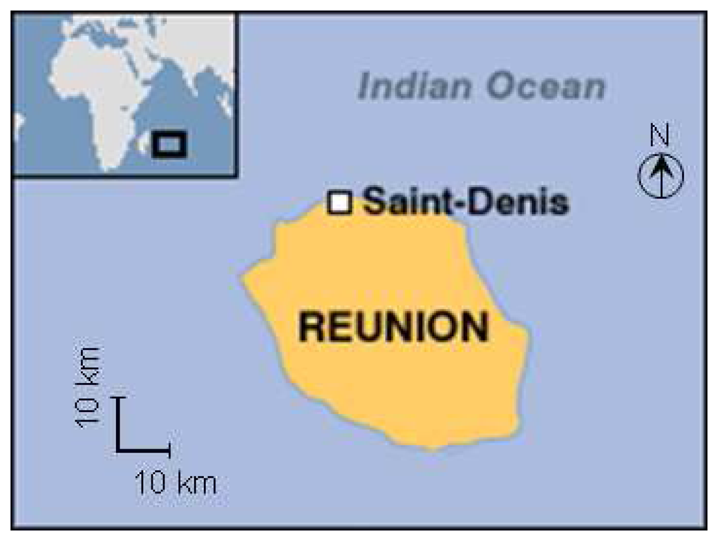
2.1. Study area

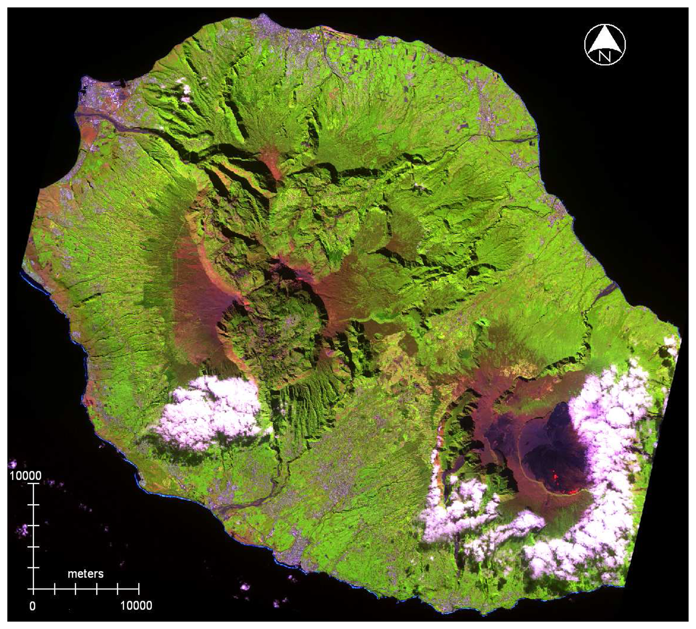
The study site is Reunion Island. It is a small territory (ca. 2512 km²) located in the Indian Ocean (21°7′ to 19°40′ S, 55°13′ to 61°13′ E), north-east of Madagascar (Figure 1). As it is located in a tropical zone, the year is divided into two seasons: a hot rainy season from November to April and a cool dry season from May to October. The island is highly mountainous. There are smooth slopes in the coastal zones, which steepen quickly toward the centre of the island. The centre is made of three cirques, which give very sharp relief.

Sugarcane is the main crop in Reunion Island. It is cultivated along the coast over 26,500 ha (Source: DDAF 2004). Most of the growers are smallholders, and the average size of a sugarcane field is about 0.8 ha. In the wet north-eastern part of the island, sugarcane is rainfed, while in the drier south-western part, it is irrigated.

2.2. Data set

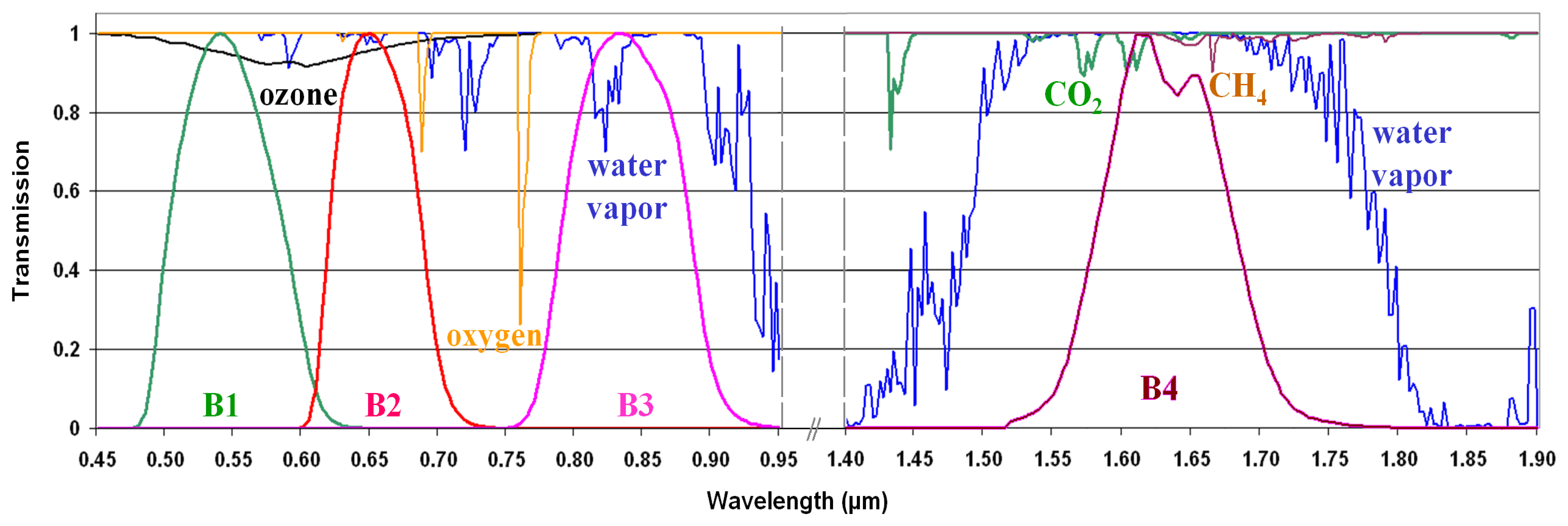
The data set used in this study consists of 18 Spot 5 images over Reunion Island (Figure 2). Both Spot 5 instruments HRG1 and HRG2 acquire radiation in four spectral bands with high spatial resolution: 10 m in the Green, Red and Near Infra-Red (NIR) bands (B1, B2 and B3 respectively), and 20 m in the Short Wave Infra-Red (SWIR) band (B4) (Figure 3).

The images belong to the KALIDEOS-ISLE REUNION database set up by the CNES¹ [23, 24]. All images are ortho-rectified and co-registered to the UTM coordinate system (zone 40 South) with a root mean square error less than 0.5 pixels per image.

Table 1. Characteristics of the imaging and atmospheric conditions of the time series. Imaging (geometric) parameters stem from image metadata. Atmospheric parameter estimation is described in Section 2.5.

Dates	SPOT 5 Instrument	Incidence angle2(in degree) (Right=-)	Solar elevation3(in degree)	Phase angle4(indegree)	Pressure5(mbar)	H2Oat6(g.cm-2)	Ozone7(cm.atm)	τ5508
01/10/2003	HRG 2	-04.65	64.10	21.28	1014	2.783	0.264	0.538
02/26/2003	HRG 1	-11.94	58.54	22.07	1013	5.469	0.259	0.322
04/24/2003	HRG 1	-04.39	48.02	40.23	1017	4.24	0.253	0.246
05/04/2003	HRG 1	10.90	46.80	47.99	1015	2.649	0.252	0.262
07/21/2003	HRG 1	10.58	41.20	53.13	1022	2.332	0.263	0.112
08/21/2003	HRG 1	18.17	48.90	51.00	1024	2.151	0.272	0.273
09/01/2003	HRG 1	-04.42	50.63	37.31	1026	1.954	0.276	0.277
10/08/2003	HRG 1	-25.95	60.40	19.75	1018	2.671	0.297	0.432
12/19/2003	HRG 1	-02.90	67.20	19.90	1017	3.093	0.272	0.357
03/17/2004	HRG 2	-19.10	54.2	25.24	1014	2.761	0.255	0.176
04/11/2004	HRG 1	+17.95	52.45	48.41	1014	4.793	0.252	0.26
05/13/2004	HRG 1	-11.80	42.90	43.86	1018	1.986	0.246	0.22
06/18/2004	HRG 2	+03.25	39.10	51.95	1024	2.357	0.237	0.11
07/09/2004	HRG 1	-04.73	38.83	49.70	1020	2.674	0.242	0.221
08/19/2004	HRG 1	+17.96	48.50	51.24	1027	2.126	0.254	0.197
10/26/2004	HRG 2	+03.30	67.90	24.94	1018	2.946	0.275	0.329
11/06/2004	HRG 1	-19.16	66.63	09.07	1021	2.541	0.286	0.351
12/07/2004	HRG 1	-12.28	66.65	11.19	1021	1.962	0.276	0.355

¹Centre National d'Etudes Spatiales (France)

²The angle defined by the direction of the satellite and the vertical to the surface.

³The angle defined by the direction of the sun and the horizon.

⁴The angle defined by the projections of the sun direction and the satellite direction on the horizontal plane.

⁵Atmospheric pressure

⁶Water vapor amount

⁷Ozone amount

⁸Aerosol optical thickness at 550 nm

shows the characteristics of the images in the time series, as well as the atmospheric data estimated at the acquisition dates. The geometric conditions of acquisition and the atmospheric components vary significantly between images.

A cloud mask was available for each image, a as well as a saturation mask that defines the positions of pixels that are saturated in at least one of the four spectral bands. A Digital Elevation Model (DEM) was provided by the IGN (BD TOPO^®) at 25 m resolution to determine the elevation of each pixel. A map of sugarcane-cultivated fields was also available.

2.3. Calculation of TOA reflectance

The images are delivered as raw numerical counts that are simply equalized (corrected for the individual behavior of each pixel detector) and corrected for digital dynamic stretching. Thus, the first step in the radiometric correction process was to compute the reflectances at the Top Of the Atmosphere (TOA) for each image. This phase takes into account a) the calibration parameters for the acquisition date, which are absolute coefficients and the analog gain values, b) the solar zenith angle and c) the normalized solar irradiance. In order to obtain physical measurements independent of the radiometer characteristics, we converted the numerical counts to radiances. The radiance L^k_TOA at the TOA is linked to the measured count X^k by the following relation:

$${\text{L}}_{\text{TOA}}^{\text{k}}=\frac{{\text{X}}^{\text{k}}}{{\text{A}}_{\text{k}}\cdot {\text{G}}_{\text{m}}^{\text{k}}}$$

(1)

where:

• A_k is the absolute calibration coefficient for band k, estimated for the date of image acquisition. This coefficient was provided by the CNES [25] for each image, and takes into account sensor degradation over time.
• ${\text{G}}_{\text{m}}^{\text{k}}$ is the analog gain of the on-board amplifier for band k [25].

${\text{L}}_{\text{TOA}}^{\text{k}}$ was then normalized by the exo-atmospheric solar incident flux in order to obtain the surface TOA reflectance ${\rho }_{\text{TOA}}^{\text{k}}$. This was calculated by:

$${\rho }_{\text{TOA}}^{\text{k}}=\frac{\pi \cdot {\text{L}}_{\text{TOA}}^{\text{k}}}{E_{\text{s}}^{\text{k}}\cdot cos{\theta }_{\text{s}}\cdot {({\text{d}}_0/\text{d})}^2}$$

(2)

where:

• $E_{\text{s}}^{\text{k}}$ is the mean exo-atmospheric solar irradiance for each band provided by the 6S radiative transfer code [7].
• θs is the solar zenith angle that stems from auxiliary data.
• d₀/d is the ratio of the Sun-Earth distance at the acquisition date to the mean Sun-Earth distance, calculated for the acquisition date by a simple ephemerid equation from 6S code [7].

To consider the effects of surface slope, cos(θ_S) in eq. 2 was replaced by:

$${\beta }_S=cos({\theta }_S)\cdot cos({\theta }_n)+sin({\theta }_S)\cdot sin({\theta }_n)\cdot cos({\phi }_S-{\phi }_n)$$

(3)

where θ_n is the surface zenith angle (slope), φ_S is the solar azimuth angle and φ_n the surface azimuth angle (aspect).

2.4. Relative radiometric normalization

We developed a simplified method for relative radiometric normalization of TOA images. This method does not require atmospheric data and attempts to uniformly minimize the effects of changing atmospheric and solar conditions relative to a reference image. The process is based on calculating linear regressions between images to be normalized and a reference one. Three main steps are identified: the choice of a reference image, the invariant targets (IT) selection, and the calculation of the linear regressions.

2.4.1. Reference image

One of the images of the time series must be chosen as a reference to which all other scenes will be related. This image must be the least cloud-contaminated, time-wise adequate for the application, and must have a good spectral dynamic range. The reference image that we chose for our normalization is that acquired on May 13^th, 2004 (Figure 2).

2.4.2. Automatic selection of IT

We developed an automatic technique for IT selection, because we wanted to make the selection process objective and obtain a sufficient number of IT covering a large spectral range.

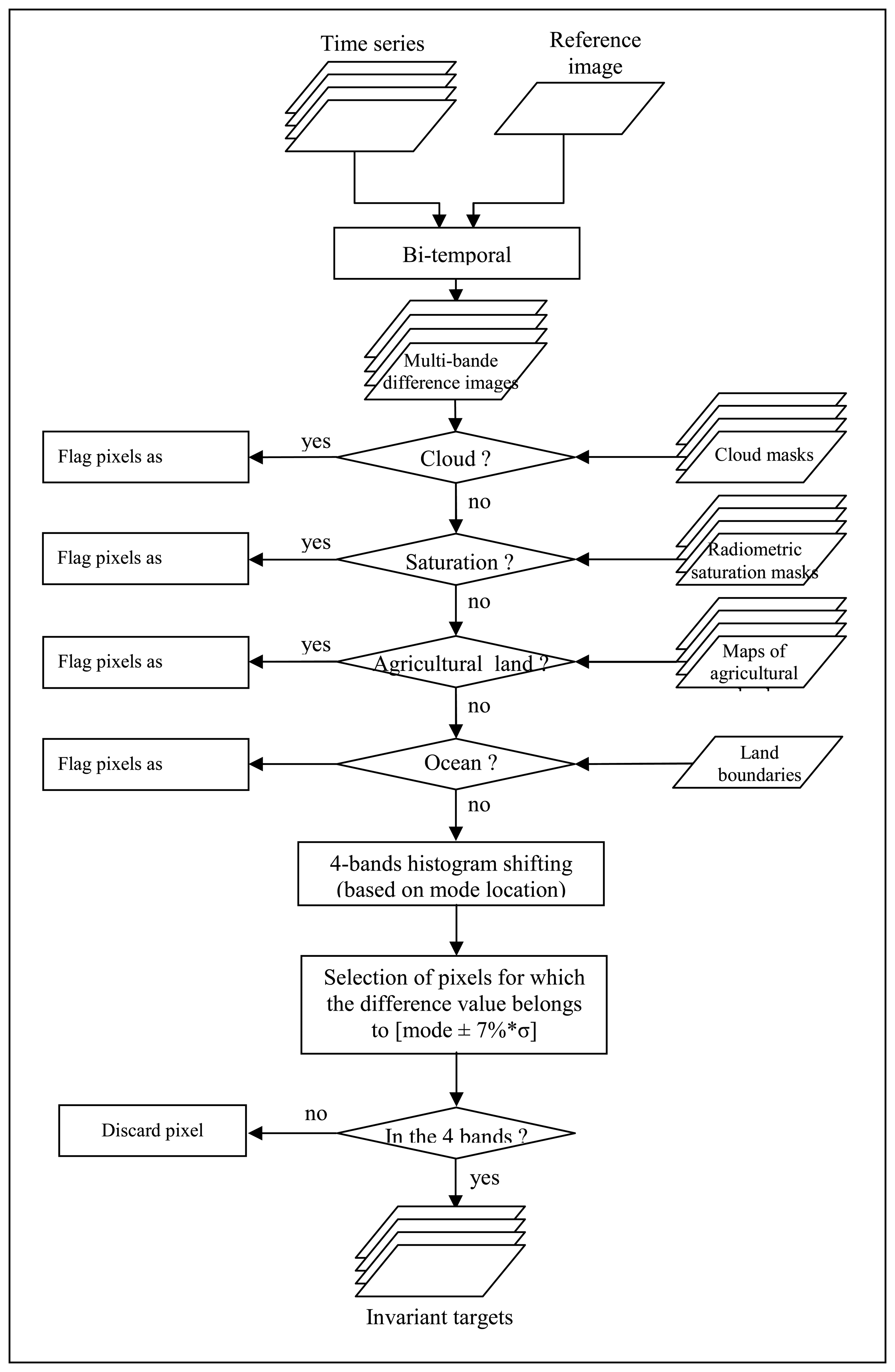
The flowchart of the automatic IT selection technique is shown in Figure 4. For each image in the time series, we first calculate a multi-band difference image (MDI) by a pixel-based subtraction from the reference image. Then we apply to each MDI a set of masks in order to discard as many changing pixels as possible. By using cloud and saturation masks, we flag pixels related to cloud and/or affected by radiometric saturation. After this, we flag the maximum number of pixels related to changing vegetation areas using available agricultural maps; the agricultural map available for this study only defines the sugarcane-cultivated fields which constitute more than 60% of cultivated areas in Reunion Island. Next, since we are not interested in having IT in the ocean, we use the land boundaries to flag ocean pixels. We then select IT for each date using the histograms of unflagged pixels in the four MDI bands.

The histogram shape of each MDI band depends on the types of changes that happen between the unnormalized image date and the reference date. Each spectral band is sensitive to different sorts of change, therefore a land cover change could cause a significant modification of pixel values in one spectral band but not in the others. In all MDI bands, the pixels with relatively slight changes will be clustered around the modes of the histograms. This means that the majority of unflagged pixels are considered targets with no or nearly no change. The difference values corresponding to these pixels differ from zero because of the change in imaging conditions from one date to another. The centre of these clusters does not necessarily correspond to histogram-band mean positions because the frequencies of changes with equal magnitudes and different signs are unequal. The rest of the histogram belongs to pixels with real land changes. These pixels may have been affected by different imaging conditions, but their effect compared to real change is negligible.

For each date, histograms in the four MDI bands are shifted so that the difference values assigned to the majorities (modes) are brought back to zero. Finally, pixels in each MDI with near null values in all four bands are considered IT. The “near null” expression was translated by 7% of the standard deviation around the histogram mode. This threshold value was chosen after several tests; it allows the selection of an optimal number of IT. We are not concerned about selecting biased invariant targets as we use selection criteria in all four bands simultaneously. The selected invariant targets represent an average of 0.044 % (10928 pixels) of the island pixels and include a wide diversity of features: pixels of large buildings, bare soils, roads, dense forests, volcanic lava, lakes, etc.

2.4.3. Regression coefficient calculations

For selected IT, we extract mean reflectance values in the four spectral bands from the TOA images. Using these values, we established linear regressions for each band of the form:

$$y=ax+b$$

(4)

where y is the reference image and x the other images in turn. The regressions were then applied to the images to perform relative radiometric normalization. By applying this method we obtained a corrected time series with relatively normalized TOA reflectances.

2.4.4. Manual selection of IT for validating the automatic selection technique

In order to validate the technique of automatic IT selection, we built up a set of manually selected IT (MSIT). This was done by photo-interpretation based on area knowledge. The MSIT set consists of 70 features of dimensions 20 m × 20 m spread over the whole island surface. It comprises large buildings, dense forests, volcanic lavas, bare soils, airport tracks, and more. MSIT were chosen so as to cover a large spectral range in each of the four SPOT 5 spectral bands.

First, we assessed the temporal stability of the MSIT by evaluating for each the standard deviation of its reflectances over all the TOA images. The mean standard deviation values of the MSIT reflectances were less than 4% in the four bands, so the set was considered acceptable.

A subset M of the MSIT was used to establish for each date a new set of linear regressions according to eq. 4, where, as before, y is the reference image (acquired on May 13^th, 2004) and x the other images in turn. This set of regressions and that obtained by the automatic selection technique were used to separately normalize the reflectances of the targets in another subset N of the MSIT. The goal is, as mentioned before, to assess the validity of the automatically selected IT. Results are shown in section 3.1, based on linear regression analysis and the evaluation of the RMSE (root mean square error) and the bias given by:

$$\mathit{\text{RMSE}}=\sqrt{\frac{1}{n}\sum {({\rho }_{\mathit{\text{Man}}}-{\rho }_{\mathit{\text{Aut}}})}^2}$$

(5)

$$\mathit{\text{Bias}}=\frac{1}{n}\sum ({\rho }_{\mathit{\text{Man}}}-{\rho }_{\mathit{\text{Aut}}})$$

(6)

where n is the number of MSIT in N, and ρ_Man and ρ_Aut are the relatively normalized reflectances of the MSIT obtained by the automatic and manual selection sets, respectively.

2.5. Atmospheric correction

The reflectance at the top of canopy (TOC) (the ground reflectance) is calculated using simulations of the 6S atmospheric correction model [7]. This code predicts the satellite signal from 0.25 to 4.0 micrometers assuming a cloud-free atmosphere. The 6S radiometric correction scheme requires a) the atmospheric pressure, which is correlated to the molecular scattering radiance, b) the gas amounts (water vapor, carbon dioxide, oxygen and ozone) for atmospheric transmittance due molecule absorption and c) the aerosols characteristics (type and concentration).

2.5.1. Atmospheric data

Gas amount and atmospheric pressure

SPOT 5 spectral bands are variably “affected” by atmospheric gas absorption and scattering (Figure 3). Stratospheric ozone absorption, with a maximum around 0.6 μm and extending from approximately 0.4 to 0.8 μm, affects bands B1 and B2. Oxygen presents strong absorption at 0.69 μm and 0.763 μm, and affects band B2 and a little band B3. Water vapor presents an absorption spectrum above 0.6 μm with more or less important absorption lines, and mainly affects band B3 and, to a lesser extend, band B2. The spectral sensitivity of band B4 to gaseous absorptions (carbonic gas, methane or water vapor) is very weak. For stable gas, such as oxygen, carbonic gas and methane, the simulations use a standard vertical profile. This profile is obtained by model US62 included in the 6S code. For more fluctuating gas, daily values are necessary. The water vapor amount, integrated over the atmospheric column, is obtained from meteorological information. We used NCEP (National Center for Environment Prediction) models to determine this parameter; the ozone amount is accessible from satellite data such as TOMS and TOAST.

The molecular radiance, resulting from light scattering by molecules, prevails for short wavelength bands (B1 and B2). Molecular radiance depends on the molecular optical thickness. This latter is well known for standard atmospheric pressure (1013 mb) and must balanced by the real pressure corresponding to the SPOT 5 acquisition date. Atmospheric pressure is also accessible from NCEP.

Aerosol characteristics

Tropospheric aerosols are the most difficult atmospheric components to characterize. The atmospheric correction code requires the aerosol optical thickness at 550 nm and a description of the particle type to derive their spectral properties.

As Reunion Island is located in the Indian Ocean, it is strongly influenced by oceanic conditions. Both L3 Standard Mapped Image of SeaWIFs products, measured over sea surrounding the island, and meteorological information from NCEP models, give the required information to characterize aerosols. SeaWIFs products give the aerosol optical thickness for a wavelength of 865 nm, while NCEP data provide the relative humidity of air. Assuming a maritime model for aerosols, we used the Shettle and Fenn model [26] to calculate the optical thickness at 550 nm from the relative humidity of the air and the optical thickness at 865 nm.

Ground elevation correction

Due to its volcanic origin, the topography of Reunion Island is strongly heterogeneous with high slopes and an elevation from sea level to more than 3000 m over only 2500 km². Since the atmospheric optical thickness fits the relief, ground elevation must be taken into account in the atmospheric correction process.

As atmospheric parameters are specified for a given altitude z_ref, their values V must be adjusted for the simulated elevations z_i. The concentrations of atmospheric components are adjusted by using scale height H applied to their vertical profiles:

$$V(z_i)=V(z_{\mathit{\text{ref}}})*exp\left(-\frac{z_i-z_{\mathit{\text{ref}}}}{H}\right)$$

(7)

The elevation correction V(z_i) (eq. 7) is applied to atmospheric pressure, aerosol optical thickness and total amount of water vapor integrated over the vertical column. The atmospheric pressure is correlated to the molecular density with a scale height of 8 km. Water vapor and aerosols are mostly concentrated in the low troposphere. Although their profiles are strongly variable, we can roughly approximate them by assuming an exponential decrease of concentration with a scale height of 2 km.

2.5.2. Calculation of TOC reflectance

TOC reflectance is deduced, pixel by pixel, by comparing measured reflectance at TOA to 6S simulations for a range of TOC reflectance using geometric and atmospheric conditions corresponding to each SPOT 5 acquisition.

The principle is based on calculating Look-Up Tables (LUTs) that give couples of TOC and corresponding TOA reflectances (one table by spectral band). The 6S code has been adapted to allow internal loops over the different TOC reflectances and, therefore, to easily calculate one LUT by spectral band. TOC reflectance varies from black ground with null reflectance to bright surface with reflectance of 0.8, with a predefined step of 0.01. From calculated TOA reflectance, we perform an interpolation in the LUTs to obtain the TOC reflectance corresponding to the measured TOA reflectance for each pixel of the image.

In order to take elevation into account, we used the DEM that gives the real elevation z for each pixel. From 6S LUTs simulated for elevations z_i and z_i+1 surrounding z, new LUTs (TOC reflectance / TOA reflectance) are calculated for altitude z by linear interpolation. Once these new LUTs are available for the current pixel of altitude z, we use it to inverse the TOC reflectance corresponding to the measured TOA reflectance.

3. Results and Discussion

3.1. Validation of the automatic selection technique of IT

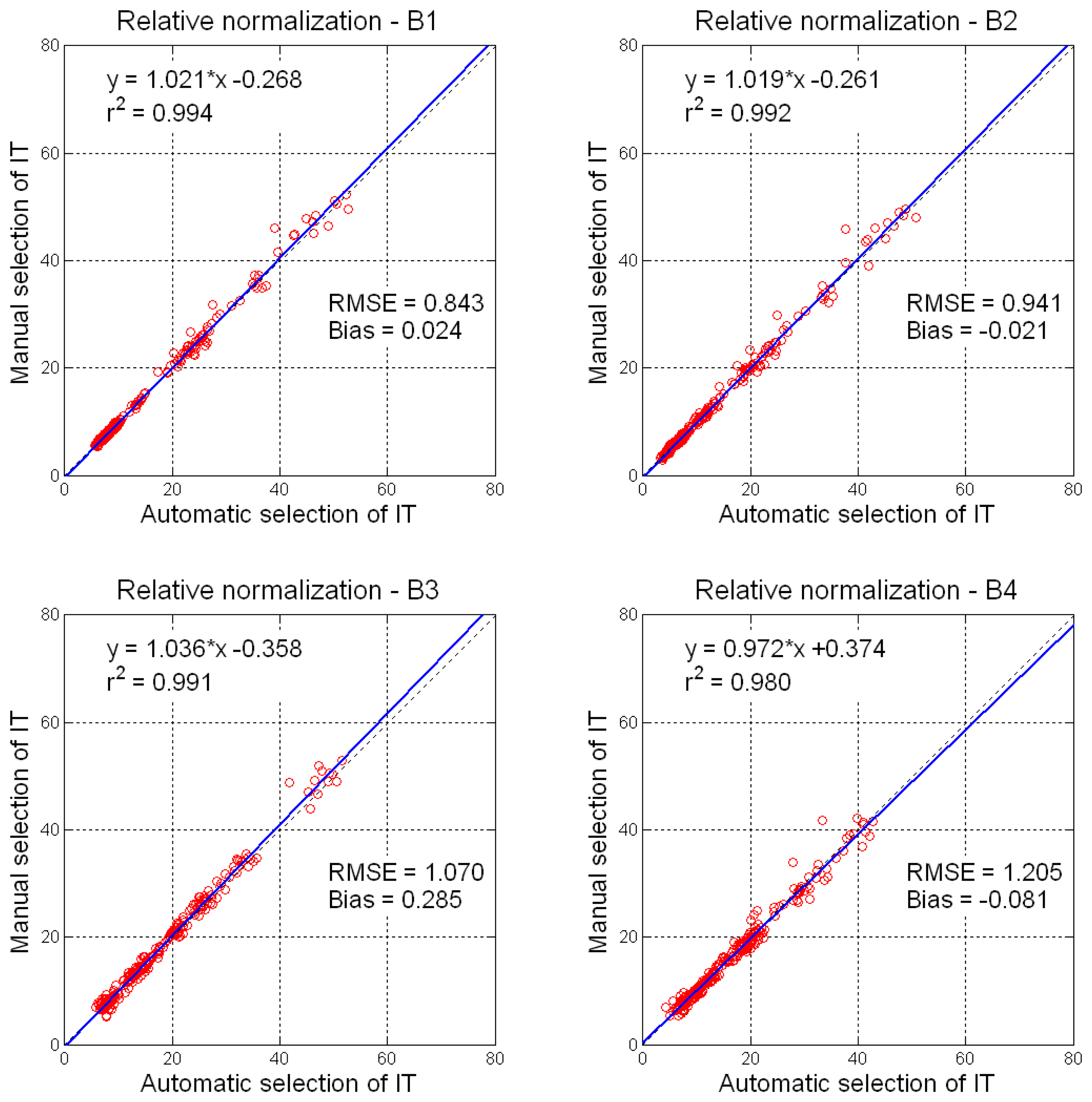
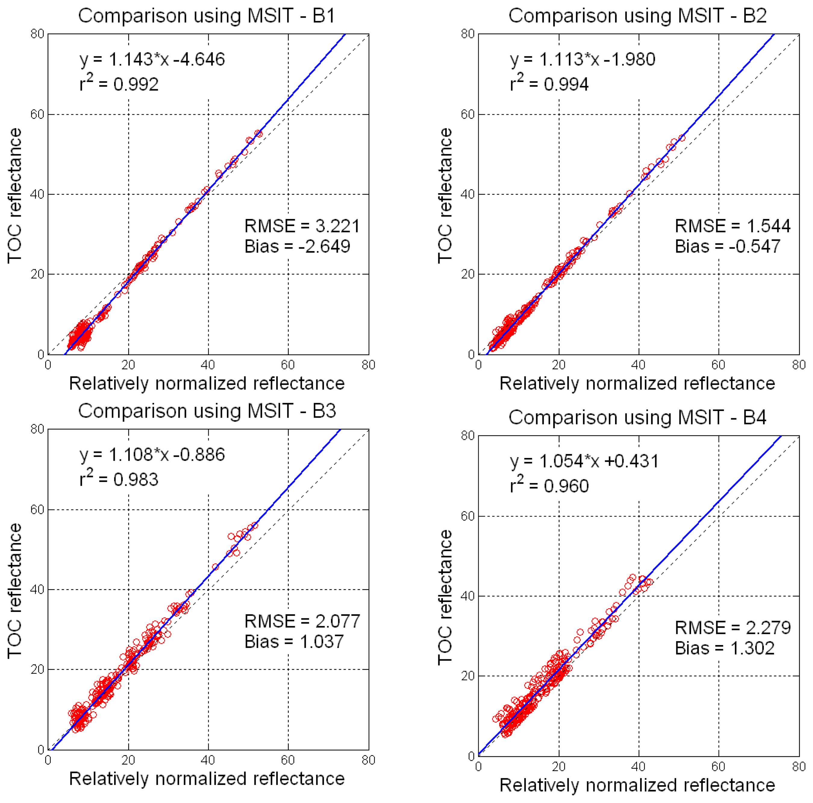
First, we present the results of validation of the IT automatic selection technique. Figure 5 shows the regressions obtained between the relatively normalized reflectances of MSIT in N (see Section 2.4.4) in the four spectral bands. The correlation between the normalization resulting from the two IT selection approaches is very strong: r² exceeds 0.98 in all spectral bands. Moreover, RMSE values range from 0.843 to 1.205, with a bias typically between -0.081 and 0.285 (very small) (RMSE and bias unit: percent of reflectance). Consequently, we consider that the proposed automatic selection technique of IT is successful and is an excellent alternative to time-consuming manual IT selection.

3.2. Comparison of relative normalization and atmospheric correction performances

The comparison between the relative normalization and atmospheric correction methods was carried out by evaluating the impact of each method on reflectances of MSIT.

For each MSIT, we extracted the mean values of atmospherically corrected reflectances (TOC reflectances) at each date. For each date, we also calculated the relatively normalized reflectances of each MSIT using relatively normalized images obtained using the automatic IT selection technique. Figure 6 shows the relatively normalized reflectances of MSIT as a function of its TOC reflectances, for all spectral bands. An excellent correlation is found in all bands: r² is equal to 0.992, 0.994, 0.983 and 0.960 in B1, B2, B3 and B4, respectively. The RMSE and bias values are small. The former ranges from 1.544 to 3.221, and the latter varies between -2.649 and 1.302.

We were also interested in evaluating the impact of each method on the temporal behavior of the MSIT reflectances. For this, we calculated the standard deviation of the profile of each MSIT over the 18 acquisition dates a) before normalization (TOA reflectances), b) after relative normalization, and c) after atmospheric correction (TOC reflectances).

Table 2. Average and maximum values (over 18 dates) of the standard deviation (STD) calculated for the reflectances of manually selected IT (MSIT): before radiometric normalization (TOA), after relative radiometric normalization, and after atmospheric correction (TOC).

	TOA				TOA+Relative normalization				TOA+Atmospheric correction (TOC)
	B1	B2	B3	B4	B1	B2	B3	B4	B1	B2	B3	B4
Average STD	1.34	1.59	1.80	2.08	0.88	1.10	1.25	1.25	1.23	1.46	1.69	1.98
Maximum STD	3.43	3.54	2.95	4.21	3.04	3.21	2.63	2.59	3.51	3.57	2.86	4.08

shows the average and maximum values of the standard deviation obtained at each level and in each band. When looking at the average standard deviations, we notice that both the relative and the atmospheric correction methods smooth the temporal profiles of MSIT reflectance in the four spectral bands. However, the relative radiometric normalization better smoothes these profiles, and also decreases the maximum value of the standard deviations (not the case for atmospheric correction). This might be due to the fact that the relative normalization corrects not only a part of atmospheric effects but also a part of surface directionality effects. Consequently, we consider that both methods reduce the radiometric distortion of the time series, but that relative normalization corrects it better.

3.3. Impact on the spectral properties of sugarcane fields

Since the final goal of this project is monitoring sugarcane crop using multi-temporal images of SPOT 5, it was necessary to assess the impact of each method on the NDVI values calculated at the sugarcane field scale. The NDVI is computed by:

$$\mathit{\text{NDVI}}=\frac{{\rho }_{\mathit{\text{NIR}}}-{\rho }_{\mathit{\text{red}}}}{{\rho }_{\mathit{\text{NIR}}}+{\rho }_{\mathit{\text{red}}}}$$

(8)

where ρ_NIR and ρ_red are the reflectances in the NIR band (B3) and Red band (B2) respectively. The NDVI temporal profile is actually a very good tool for sugarcane yield prediction and harvest detection [27-29].

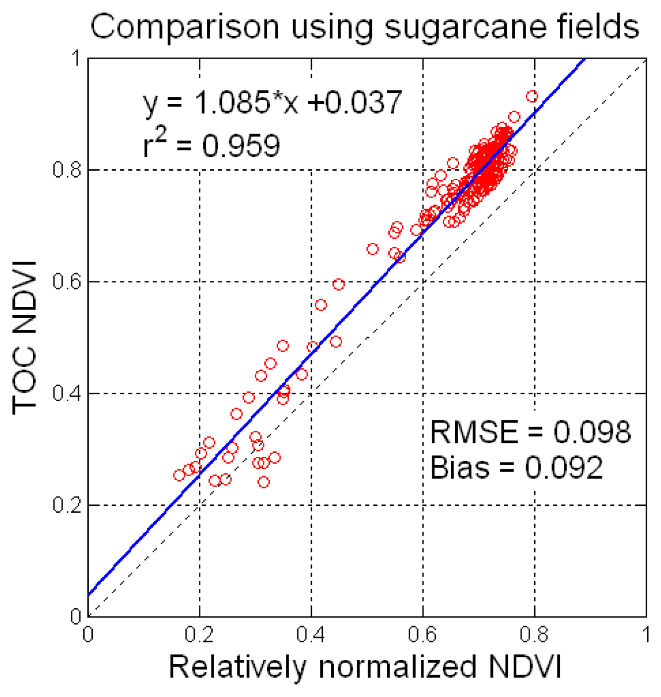
Twenty fields were chosen for the comparison. We calculated for each field the mean NDVI values at each date using relatively normalized images and TOC images.

Figure 7 shows the regression obtained between the relatively normalized NDVI and the TOC NDVI values obtained for all dates and fields. There is a strong correlation (r² = 0.959) between the two methods. However, the RMSE and bias values are non-negligible (RMSE = 0.098, Bias = 0.092). The relative error was estimated to be 12.66%, which is high.

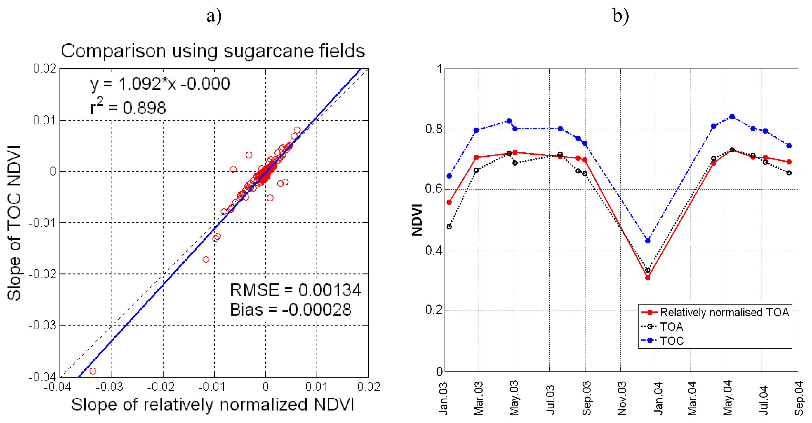
Since relative radiometric normalization is not intended to absolutely correct the images but only to normalize them according to a reference image, it was more relevant to compare the relative evolution (increase or decrease) of NDVI from one date to another. Thus, we compared NDVI slope values calculated for each couple of consecutive dates for all fields (see Figure 8a). We notice a good correlation (r² = 0.898) and low RMSE and bias values (0.00134 and -0.00028, respectively). Only 4% of the points were significantly spread along the regression. This means that globally both methods lead to a very similar behavior of NDVI. Looking more in-depth at each field case, we see that NDVI patterns obtained by the two methods are very comparable but sometime differ in a critical stage of the crop cycle. Figure 8b shows the temporal profile of NDVI obtained for a sugarcane field using TOA reflectances, relatively normalized reflectances and TOC reflectances. We can see that the relative normalization smoothes the NDVI profile more than atmospheric correction. For instance, the NDVI fluctuation that appears in May 2003 on the TOA and the TOC profiles does not appear on the relatively normalized one. Slight differences are also noticed in the senescence stage, i.e. the stage after maximum growth. These differences can lead to different interpretations of the crop state. For example, when looking at the TOC NDVI pattern between June and October 2004, we conclude that the sugarcane has dried remarkably because the NDVI decreases by 0.1, but the 0.04 decrease of the relatively normalized NDVI does not indicate the same. Since no ground truths are available for comparison, we cannot conclude one or the other. What we can say at this stage is that relatively normalized NDVI patterns obtained by the two methods are very comparable, but slight differences might have an impact on derived crop indicators that need highly accurate data.

4. Conclusion

In this paper, we addressed the issue of normalizing the radiometry of a SPOT 5 time series acquired over Reunion Island, and introduced an automatic method for relative radiometric normalization based on the reflectances of invariant targets. Since finding these targets is an important step, we developed and validated an automatic technique for IT selection. The main advantages of this method are its implementation simplicity, its automaticity, its applicability to images acquired in different seasons and the fact that it does not need atmospheric data; however, results depend of the selected reference image.

We also presented an atmospheric correction method based on the 6S model and described the retrieval of atmospheric parameters. This method corrects absolutely the atmospheric effects on the radiometry whatever the date and site. Nevertheless, it is difficult to quantify atmospheric data at the local scale since atmospheric parameters are often provided at the global scale. Another important limitation is the fact that bidirectional reflectance effects are not corrected.

We compared the performance of both methods using a set of manually selected invariant targets; this comparison shows very strong correlation and low error rates. Both methods reduce the radiometric distortion of the time series, but relative normalization gives better results.

Impact analysis of the methods on the NDVI of sugarcane fields showed strong correlation between normalized values, although the observed error rate was relatively high. Very comparable NDVI patterns at the field scale were obtained, but slight critical differences were observed that might influence the computation of phenological and production indicators.

In conclusion, we consider that the developed relative normalization method can globally be a good alternative to atmospheric correction when working with high spatial resolution multi-temporal imagery.