Relocating Sensor Nodes to Maximize Cumulative Connected Coverage in Wireless Sensor Networks

SIK University, Department of Information Technologies, Sile, 34980, Istanbul, Turkey
Sensors 2008, 8(4), 2792-2817; https://doi.org/10.3390/s8042792
Submission received: 31 March 2008
/
Accepted: 18 April 2008
/
Published: 21 April 2008
Abstract
:In order to extend the availability of the wireless sensor network and to extract maximum possible information from the surveillance area, proper usage of the power capacity of the sensor nodes is important. Our work describes a dynamic relocation algorithm called MaxNetLife, which is mainly based on utilizing the remaining power of individual sensor nodes as well as properly relocating sensor nodes so that all sensor nodes can transmit the data they sense to the sink. Hence, the algorithm maximizes total collected information from the surveillance area before the possible death of the sensor network by increasing cumulative connected coverage parameter of the network. A deterministic approach is used to deploy sensor nodes into the sensor field where Hexagonal Grid positioning is used to address and locate each sensor node. Sensor nodes those are not planned to be actively used in the close future in a specific cell are preemptively relocated to the cells those will be in need of additional sensor nodes to improve cumulative connected coverage of the network. MaxNetLife algorithm also includes the details of the relocation activities, which include preemptive migration of the redundant nodes to the cells before any coverage hole occurs because of death of a sensor node. Relocation Model, Data Aggregation Model, and Energy model of the algorithm are studied in detail. MaxNetLife algorithm is proved to be effective, scalable, and applicable through simulations.
1. Introduction
A Mobile Wireless Sensor Network (WSN) is a collection of sensor nodes deployed in a surveillance area to extract information; where each sensor node has sensing, processing, communication, and locomotion capabilities [1]. Each sensor node is capable of sensing events, execute some processing on the sensed data, communicate with neighbor nodes, and change position when it is required. The main purpose of deploying a sensor network to a surveillance area is to get as much information as it is possible, before the sensor nodes, and eventually the whole network dies. While trying to reach this goal, the researchers struggle with the two constraints: energy scarcity, and low computation capacity of the sensor nodes. When wireless sensor networks were initially introduced, mobility was not tailored to the primitive sensor nodes [2]. As the research in this area emerged in years, the requirements for the WSN applications are improved as well as the capabilities to satisfy those requirements. Mobility is possibly the most important among all. Mobility studies targeted for gaining advantages such as:
- Enabling connectivity of clusters when there is a hole between the mainland and the islands
- Increasing coverage of the cluster by relocating redundant nodes to the holes
- Fine-tuning the sensor nodes within a cluster when better coverage and connectivity can be performed after relocation
- Healing the network by connecting the islands to the mainland by the migration of sensor nodes
Mobility of sensor nodes to fill in a coverage hole is introduced, and studied by some researchers [3-11]. These studies mainly concentrate on finding the most appropriate sensor node around to fill in a gap just realized. Common features of the studied algorithms are:
- They concentrate on solving one problem at a time, hence not scalable.
- Distributed algorithms, those run on all sensor nodes are used without much help of the cluster head or sink; results in early power exhaustion of sensor nodes.
- Distributed algorithms will also possibly result in many nodes relocating to the same hole, hence causing overlapping.
- The relocation activity starts after the death occurs; hence creating delay to fill in the hole.
- The algorithms include only the relocation activity, and do not include how the regular works are to be performed concurrently by the sensor nodes; hence are inapplicable.
- Too much message traffic between the cells in need of extra sensor node, and many sensor nodes which may relocate potentially to fill in the hole; hence causing too much energy consumption, overhead, and poor data aggregation.
- Their complexities are high.
We introduce MaxNetLife algorithm, which essentially solves the deficiencies of prior algorithms, and also add some additional features. Each player, namely the sink, cluster heads, and the sensor nodes have their own roles in the algorithm. Data traffic is managed by the cluster head, and excess message traffic is prevented. The algorithm contains all the work done by the sensor nodes, hence it is inclusive. Energy model of the sensor nodes, Relocation model of the sensor nodes, as well as Data Aggregation model of the network are studied as part of the algorithms, hence it is inclusive. An open-source simulation environment, called MobilSim is designed and implemented to be used in simulating our model using Java programming language. MaxNetLife algorithm is tested extensively through the created test bed.
The rest of the paper is organized as follows. Chapter 2 provides the definitions and the related work. In chapter 3 our new proposed MaxNetLife algorithm, which maximizes the cumulative connected coverage through mobility is proposed. The performance analysis of our algorithm is analyzed in chapter 4. Chapter 5 points out the contributions of our algorithm, and concludes our paper.
2. Definitions and Related Work
Two important hardware components of sensor nodes are sensors and transmitters. The sensing ranges of sensors define the coverage; whilst the transmission & reception ranges of transmitters define the connectivity of the sensor network. It is important to provide connectivity and coverage at the same time, since a sensed data is not good if it can not be sent to the sink because of the poor connectivity. After sensor nodes are deployed to the surveillance area, no problem regarding coverage or connectivity may be realized initially, and the same ideal situation may even go for a long period. But, it is a fate that some nodes, and probably the ones closer to the sink will start to die, so that the sensed information won't be transferred to the sink. A cell which does not include any node is called as coverage hole, or briefly as hole. Another term, gap is used to refer to this situation in some works. A hole may also consists of more than one vacant cell, which of course is a bigger problem. Holes may start to occur much earlier then expected when a poor design is used, a poor deployment occurs, or a high amount of energy is consumed.
Coverage of the WSN is designated by the collection of sensing units of the sensor nodes, whilst the connectivity is designated by the transmitters. The mainland is part of the network which contains the sink together with the sensor nodes those are connected to the sink, either directly or via other nodes. Sensor nodes in a mainland can send their messages to the sink, by definition. An island in the network contains one or more nodes which are not connected to the sink; hence, they can send messages to each other, but can not send any message to the sink. A network is connected if every node in the network is part of the mainland, not connected if at least one island exists.
The coverage of a sensor node is not of importance, until the node can send its data to the sink, which requires that the sensor node must be connected to the sink, in other words be a part of the mainland. Thus, coverage is not beneficial until connectivity is accomplished. Without a valid route path between the sender (node) and the receiver (sink), a sensed data is worthless. Hence, connected coverage is useful, while unconnected coverage is one of the basic problems in WSNs.
Sensor nodes have limited energy capacity, and recharging batteries is impractical, if not impossible. Therefore, energy-related study has become an area of intense research activity. [12], for example tries to decrease number of messages sent by the sensor nodes in order to decrease energy consumption within the network. Researches those concentrate on the design goals of sensor networks mainly put forward the importance of maximum coverage [13-15] as well as prolonged network lifetime [16-17]. Embedding the concerns about connectivity, coverage and lifetime all together into one simple parameter would help much to analyze performance of a given network.
We propose to use a new design parameter, namely cumulative connected coverage; which can be explained as the combination of all three parameters. Informally, it can be defined as maintaining connected coverage for an extended period of time. Formally, Equation (1) can be used to calculate its value. Ct is the marginal connected coverage at t = ti, and CC is the cumulative connected coverage of the network through network lifetime.
Many researches are performed on how to find the best way to arrange given number of sensor nodes to maintain maximum possible coverage. [13] is one of those, and confirms that the hexagonal model gives optimal performance in terms of requiring minimal number of sensor nodes for a given sensor field. SENDROM [18] proposes individual sensor nodes to be deployed around to be used in disaster recovery using sensor networks, where data collecting nodes, called cnodes, are used as the cluster heads. A distributed data aggregation and dilution technique, called DADMA is proposed in [19] for sensor networks where nodes aggregate sensed data to the cluster.
In this study, sensor fields are divided into clusters, and clusters are further divided into hexagonal cells. When only one node is enclosed within a cell, it is called as master node, and it will be responsible to perform the activities within that cell. If more than one node exists in a given cell, one of the nodes will be referred as the master node, and the others will be referred as redundant nodes. We further classify redundant nodes as either extra node or excess node, depending on their future possible usage in or out of the cell. If a redundant node is planned to be used in the same cell after a while, after the master node dies for example, that node will be referred as extra node, and will be kept within the same cell for future usage. Redundant nodes those are not planned to be used in the current cell are called as excess nodes, and existence of excess nodes in a cell, especially for a long period is against productivity.
Coverage is an important criterion for the quality of service in a sensor network, and handling the coverage holes received significant attention [4]. One approach is to deploy vast number of redundant sensor nodes to the cells. In [5], extra sensor nodes are deployed randomly in the area to be monitored if deployed sensor nodes can not achieve the required coverage. In order to maximize coverage and connectivity, some sensor nodes must be relocated to fill the holes by using mobile nodes. As also stated in [6], locomotion facilitates a number of useful network capabilities, including the ability to self-deploy and self-repair. Relocating excess nodes to cells in need of sensor nodes improves productivity.
When a hole occurs, the obvious solution seems to relocate the closest redundant sensor node to heal the coverage hole. How to find the closest excess node may seem trivial at a first glance, but unfortunately it is not so. It has been pointed out that there are indeed important issues to consider such as minimizing total energy consumption, minimizing completion time of the overall movements via cascaded relocations of several sensor nodes, and minimizing average moving distances in cascaded relocations of several sensor nodes etc. [3].
Mobility of sensor nodes to fill in a coverage hole is studied by the researchers. Not only minimizing the distance to relocate, but also reducing the difference of the remaining energy among sensor nodes is studied in [7] for a longer system lifetime. In [7] it is aimed to find the positions and movement information of nodes to achieve maximum coverage and to form a uniformly distributed wireless network in minimum time and with minimum energy consumption. Hence, [7] concentrates on only proper localization of sensor nodes after deployment and does not consider the latter relocation requirements.
In [8] a self-organizing technique for enhancing the coverage of wireless sensor networks after initial random placement of sensor nodes is proposed, which can not appropriately handle simultaneous relocations. One of the weak points is the possibility that more than one sensor node may move towards the same location. This problem is tried to be solved by inserting a delay time, hopefully different for each sensor. Another problem with this study is execution of the same algorithm by each individual sensor nodes in every possible opportunity, resulting in extra energy consumption.
In [3], matching redundant sensor nodes to the coverage hole is managed in publish / subscribe fashion. The most possible reason for using a publish / subscribe algorithm is considering the matching problem as a rare case. As a matter of fact, this is a frequent case.
In order to increase coverage by healing the coverage holes, vector based (VEC), Voronoi based (VOR), and Minimax algorithms are proposed in [9-10] which uses mobility of sensor nodes. The two problems with [9-10] as pointed out by the same research group in [3] is that moving neighbor mobile sensor nodes may create new holes in that area; and it takes a long time for the algorithm to terminate. Authors propose finding the locations of the redundant sensor nodes first, and then to design an efficient route to move to the destination in [3]. We don't assume that the new approach solves the problem as effectively as required, since it does not contain a deterministic approach to select the most appropriate node to fix the hole. We will address this issue further in this study.
Authors of [11] propose four Dynamic Coverage Maintenance (DCM) schemes that exploit the limited mobility of the sensor nodes. Maximum energy based (MEB) preferentially moves the neighbor having maximum energy among all eligible neighbors; MinMax Distance (MMD) tries to minimize migration distance; Minimum D/E (MDE) combines the objectives of the MEB and MMD by choosing the node with the least ratio of the maximum distance each neighbor can move to their available energy (D/E); Minimum Distance Lazy (MDL) moves the closest neighbor.
After a detailed analysis of earlier works, we list some work those need to be implemented in this area as follows:
- Earlier works working on mobility solves one assignment problem at a time; which does a many-to-one mapping of sensor nodes at a time. The actual problem includes many coverage holes as well as many redundant sensor nodes in each cycle; hence a many-to-many problem exists.
- If the relocation activity starts after the death of a sensor node creating the hole, a time delay will definitely happen. Since the delay will occur in almost all relocations, a healthful network process will not occur. It is more efficient to preemptively relocate a redundant node to a location just before an expected death of a sensor, and in some applications this approach may be even crucial.
- Data transfer model between the dying sensor node and the relocating sensor node is an important issue for the broad picture.
- The content of the data package is very important and should be clearly addressed.
- Sensor node relocation algorithm is not a stand-alone activity. The regular activities of the sensor nodes should continue concurrently while the relocation activity is performed.
- The relocation activity indeed demands a more detailed study, including:
- ○
- There may not be any redundant sensor node available.
- ○
- The distance between the coverage hole and the most available redundant sensor node may not justify the relocation, most possibly because of the required energy consumption for relocation. The sensor node may consume most, if not all, of the remaining power if it performs the task; hence not satisfying the relocation.
- ○
- The possible relocation direction of a redundant sensor node may be contrary to general power consumption within the network. For example, the cluster containing the redundant sensor node may be in fast power reduction phase, and most possibly that cluster may complain coverage hole in a close future.
- Relocation requirement may be caused by dynamic change in the mission of the sensor network. Some area, not included in the initial design, may be added to the region of interest (ROI) requiring group relocation of sensor nodes. [20] partly addresses this issue by Reference Point Group Mobility (RPGM).
3. MaxNetLife Algorithm
3a. Motivation / Key Points / Fundamentals of our algorithm
The primary motivation of our algorithm is increasing CC, cumulative connected coverage ratio, of the WSN. It is mentioned above that, in order to reach this goal, maximization of connected coverage as well as extending network lifetime at the same time is required, both of which largely depends on low energy consumption, meanwhile appropriately utilizing the consumed energy.
In our algorithm, we consider the following parameters:
- (1)
- Priority: Some regions in the surveillance area may have higher priority over others. When a redundant sensor node is to be relocated, holes within a region with higher priority should be chosen, based on the fact that all other parameters are equal. The priority may be imposed by the design parameters, or it may have some technical requirements such as continuously establishing data corridors among specific regions, or between specific cluster and the sink, for example.Methodology for assigning priorities to different regions or clusters mainly depends on the properties of projects. As an example, the boundary of the area may have higher priority than the inner regions in a security surveillance system. At first glance, dense deployment into regions with high priorities seems a solution to handle the priority management; which has some drawbacks. The first one is that it works only for static priority definition. Priorities of regions may also change dynamically after the deployment phase. As the possibility of an attack direction changes, the segment of the nodes with high probability may change for example. This implies that the solution in defining and processing priority must be embedded into the algorithm to process it dynamically. Handling priority dynamically in our algorithm increases flexibility and adaptability, without sacrificing efficiency. Our priority scheme mainly helps us strengthening the more important sub regions / clusters dynamically.
- (2)
- Scarcity: If number of sensor nodes in a cluster is reduced below a threshold level, the sensor nodes may create an island which becomes disconnected from the mainland. Migrating all sensor nodes to another cluster may be reasonable in this case.
- (3)
- Being comprehensive: Previous works are concentrated on individual problems. Some tried to relocate sensor nodes to initially locate them into their design locations after initial deployment, but did not care about latter issues. Others tried to heal coverage holes, but concentrated on only one specific hole at a time. These types of works tried to solve either many-to-one problems, such that selecting the most appropriate redundant node to relocate and heal one such hole, or one-to-many problems, such that selecting the most appropriate hole to cover by an individual redundant hole. None of them worked on extensive many-to-many assignment problems. Our algorithm does not only solve individual problems, but also handles all relocation issues throughout network lifetime. It handles the relocation requirements starting with the deployment, resuming with relocating sensor nodes to heal the coverage holes throughout network lifetime until the death of the whole network.
- (4)
- Adaptability to changes in the mission statement: The algorithm should be robust for possible changes in mission parameters such as shift in location of the surveillance area, or changing priorities of different clusters. Sensor nodes may be required to move not only for healing the coverage holes occurred in the network, but also for satisfying the updated mission requirements.
- (5)
- Data transfer: In order to maintain continuity in data collection, the sensor node which relocates to a hole must receive the data of the dead sensor node. There are some options to transfer data between predecessor and the successor nodes:
- (a)
- If the successor node arrive the hole before the predecessor die, the predecessor transfers all data that it owns to the successor node after the relocation.
- (b)
- If the predecessor node dies before successor arrives, it transfers data either:
- to the cluster head, or
- to one of its neighbor sensor nodes, which we call as safe node.
- (6)
- Concurrent processing: Relocating sensor nodes execute the relocation part of our algorithm during the migration, while other sensor nodes execute regular tasks such as sensing, analyzing, transmitting etc. Thus, relocation issues and regular tasks are processed concurrently. This is an improvement over the previous studies in this area, since how the relocating and stable sensor nodes behave are not made clear in those works. In our algorithm, only relocating sensor nodes are distracted with the migration, whilst all other sensor nodes continue to execute their regular mission without any interruption. This capability apparently increases network efficiency.
- (7)
- Power Consumption Rate: Our algorithm introduces power consumption rate (pcr) of the clusters, which shows the average energy consumption in the last T period of time. The sink calculates pcr of each cluster in each period, and uses it to preemptively relocate sensor nodes to the cluster which will require node support in a close future. Sink also uses pcr of each cluster to predict a possible scarcity event from being occurred, and help the cluster head to which cluster should the sensor nodes migrate.
- (8)
- Uniformity: In addition to maintain connected coverage in a high success level, our algorithm can be used to smoothen sensor node distribution among clusters when excess number of sensor nodes are initially deployed in some regions, where scarce deployment rate exist in others. Uniformity will enable utilization of energy more efficiently, since even distribution of sensor nodes ease the efficiency of algorithms [21]. Some clusters may be intentionally overloaded by redundant sensor nodes, as it will be described in the following paragraph in detail.
- (9)
- Preemptive relocation: Our algorithm enables relocating redundant sensor nodes to the locations where power consumption rate is high. If other parameters are kept same, the sensor nodes closer to the cluster head are expected to consume more energy, because they will be required to relay many messages [22]. Hence, those locations are candidates to require redundant sensor nodes for continuity. In our algorithm, redundant sensor nodes are migrated to the places where power consumption rate is high, in which coverage holes are expected to occur in close future. These sensor nodes wait in standby mode until an active node fails for some reason, after which it switches to on mode. This preemptive approach reduces the period between the death of the predecessor node and the arrival of the successor node, even makes it a negative value by relocating the successor node before the predecessor node dies.
- (10)
- S.O.S handling: The algorithm should contain an emergency recovery plan for isolated sensor nodes that can not communicate with the mainland. Every sensor node should be able to run the recovery algorithm in such a case to migrate to a position where it will be connected to the mainland back again. This algorithm prevents the possible loss of the sensor node which is caused by death of neighboring sensor nodes and / or the cluster head, or relocating to a rural district for some reason.
3b. Assumptions
Followings are the assumptions on the sensor nodes made in this study:
- All nodes are identical to each other, in terms of:
- ○
- Initial energy level and energy consumption rate for each action,
- ○
- Sensing range,
- ○
- Communication range,
- ○
- Programs loaded into the memory.
- Nodes know their positions.
- Nodes have locomotion capability with a reasonable speed to perform the algorithms stated in this work.
- Nodes are organized as clusters and the cluster heads perform data aggregation before sending aggregated data to the sink. Nodes do the sensing and relaying of data packets to the cluster heads, and cluster heads perform data fusion and relaying of data packets to the base station.
- Shape of sensing and communication circle of sensor nodes are not perfect. This truth, in practice, means that sensor nodes have minimum and maximum affective ranges, depending on the technical properties of the sensor node equipments and the environmental conditions. Being aware of this, we are interested in only the minimum affective ranges for both sensing and communication, and use that value in our algorithm.
- Time synchronization of the sensor nodes is performed.
Followings are the assumptions on the cluster heads made in this study:
- Cluster heads have enough transmission range so that they can communicate among themselves.
- Cluster heads have much higher processing capability, power, and storage capacity than sensor nodes so that the constituting algorithm can be processed.
- Each cluster head utilizes a database which consists of all of the necessary information about sensor nodes within that cluster.
- Cluster heads constitutes mobility of sensor nodes within the cluster, compute the power consumption rate of each individual sensor, predict the possible dissipation/death of each individual sensor, and arrange migration of a sensor node to that point, or request help from the sink when extra sensor nodes are required.
- Arrange the data transfer between the former and the latter sensor nodes, undertake the valuable data if the former will be possibly dead before the latter sensor node arrives
- They must be positioned in appropriate locations to manage the sensor nodes in the cluster.
3c. Creation and Addressing of the Sensor Network
In this study, the clusters will be referred with their Cluster ID starting from 0. Each sensor node in a cluster will have its unique ID, also starting from 0. Sensor nodes will be identified with the Cluster Id that it belongs to, together with the Node ID of the node within that Cluster.
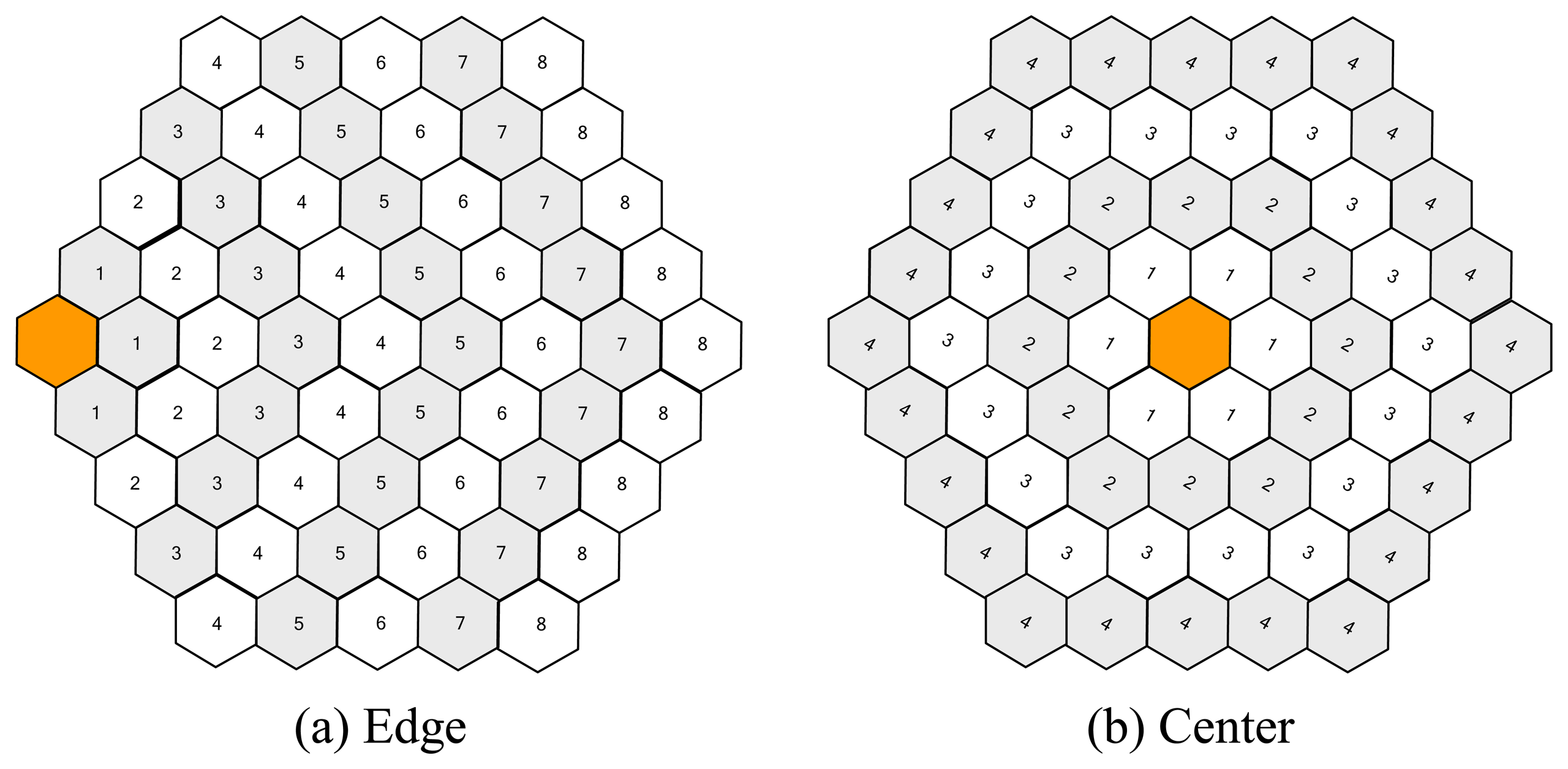
Because of higher success in providing coverage with the same amount of sensor nodes, we use hexagonal grid cell representation for locating sensor nodes within clusters. The placement of cluster head within the cluster is also an important issue in hexagonal placement of sensor nodes. Figure 1 shows two extreme alternatives for positioning cluster heads. We suggest each sensor node sends its data to its neighbor cell in the inner tier, which enables sending data with minimum possible number of hops among other alternative transmitting routes. Each sensor node in Figure 1 is marked according to number of hops required to send a message which is originated from that sensor node, to the cluster head. The three neighbors of the cluster head can send a message to the cluster head directly, hence it requires only one hop. This is why all neighbors of the cluster head is marked with “1”. The sensor nodes marked with “2” can send messages to their neighbors those are marked with “1”, and transferring data to the cluster head requires 2 hops. All other sensor nodes will have similar behaviors, so that the cost of message transfer from farthest sensor nodes, which are marked with “8”, requires 8 hops. Assuming that each sensor node sends one (periodic) message to the cluster head in each period, total number of hops for sending all messages to the cluster head in one period can be calculated as 3.1 + 5.2 + 7.3 + 9.4 + 9.5 + 9.6 + 9.7 + 9.8 = 304. The cluster head is positioned on the center in Figure 1(b), and the sensor nodes behave similarly as described in previous statements. The 6 innermost nodes require 1 hop, 12 nodes in the next circle requires 2 hops etc. Number of required hops in this case is calculated as 6.1 + 12.2 + 18.3 + 24.4 = 180, which is far less than the previous alternative.
By looking at Figure 1(b), we can easily observe that, the nodes in the inner tiers are bound to make more hops than the nodes in the outer tiers. Thus, the outermost nodes will consume least, and the innermost nodes will consume highest amount of energy when equal number of messages are to be sent by each node to the cluster head. This result is not surprising, and is in accordance with many studies made for the existing routing algorithms such as [22].
This information has a simple reflection to our algorithm. We locate redundant nodes in the cells in inner tiers of each cluster; they wait in standby mode and relocate to the places where nodes exhaust their energy. This solution is also harmonious with the results of [22]. By looking at the number of hops required for equal frequency of message creation, if x number of nodes are required in the outermost (4th) tier, 2x nodes are required in the 3rd, 3x nodes are required in the 2nd, and 4x nodes are required in the 1st, or the innermost tier. Thus, 10% of nodes need to be inserted into the 4th, 20% into the 3rd, 30% into the 2nd, and 40% into the 1st tier. We call this placement method of sensor nodes as heuristic deployment, and we compare its success against uniform deployment where each cell consists of same amount of sensor nodes in simulation analysis.
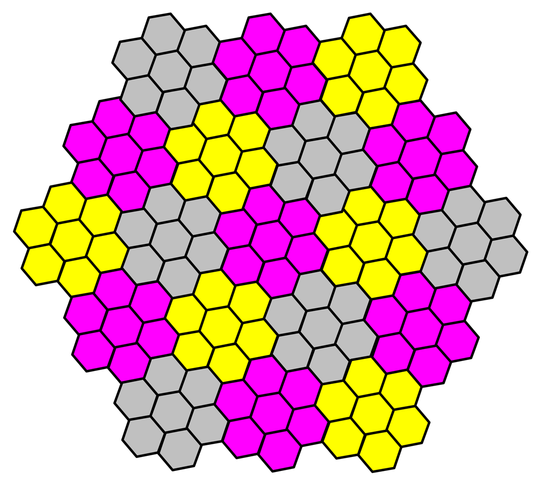
By noticing the charm regarding the advantages of hexagonal positioning of sensor nodes within the clusters, and recognizing that similar advantages will be valid for positioning clusters within the sensor field, we choose to hexagonal grid system for cluster design too. Building hexagonal clusters with sensor nodes those are also positioned in hexagonal cells provides (1) an easy data acquisition scheme (2) proper utilization of data acquiring, (3) scalability, and (4) consistent structure. Figure 2 consists of a cluster which is built in as a hexagonal shape, consisting of 61 hexagonal cells. The required number of hops to send one packet from each cell to the cluster head is 180, as calculated before. Figure 2 consists of two different configurations, and there is practically no difference between both. Figure 2 shows the structure of the complete sensor field with sample amount of clusters as well as sensor nodes in the clusters. Hence, the clusters are formed in hexagonal shape as well as sensor nodes within the clusters.
3d. Relocation Model: Filling the Hole by Sliding Model (FHSM)
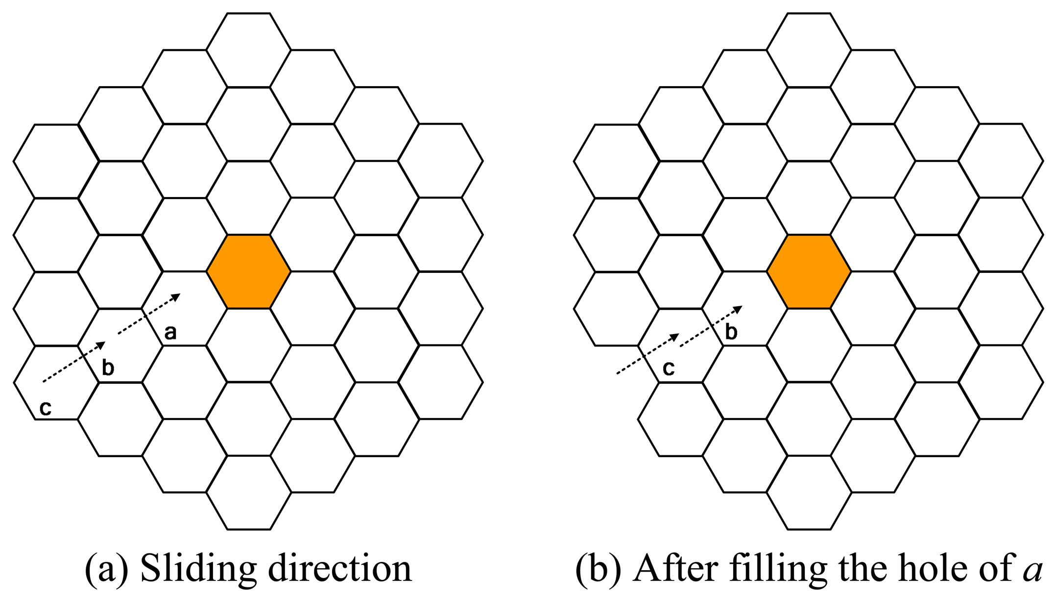
This algorithm provides continuous connectivity of the sensor nodes within each cluster by filling out the coverage holes using the sensor nodes within the neighbor cells. When a master node dies in a cell, one of the redundant nodes will become master node, if exists. Otherwise, a coverage hole occurs. In this case, a sensor node from the neighbor cell relocates to the coverage hole. If there is a redundant node exist the neighbor cell, then that node relocates. Otherwise, the master node in the neighbor cell relocates. Hence, connectivity of all sensor nodes within the cluster is satisfied continuously. Figure 3 shows which sensor nodes should relocate to fill in the hole in the inner tier. If cell a creates a hole, a node from cell b fills in the hole; a node from cell c fills in the hole if the master node in cell b moved to cell a, resulting in creating a hole in cell b. We use the term sliding for filling out the hole in the inner cell by a node from the outer cell. After consecutive sliding relocations happen, a hole may occur in the outermost tier as can be seen in Figure 3(b), and hence relocation from other clusters may be required to fill the holes in the outermost tier of the cluster. Please remember again that after the master node in cell a dies, sliding is not required if a redundant node exists within the same cell, where the redundant node just wakes up to be the master node afterwards.
3e. Data Aggregation Model: Data Acquisition by Partitioning Model (DAPM)
According to our hierarchical communication model, all sensor nodes forward their messages to the head of the cluster in which they belong to, via the pre-determined neighbor nodes. Cluster heads have higher communication range capacity, which allows them to send the accumulated data to the sink via other cluster heads, instead of using sensor nodes. This structure enables both simplicity and efficiency.
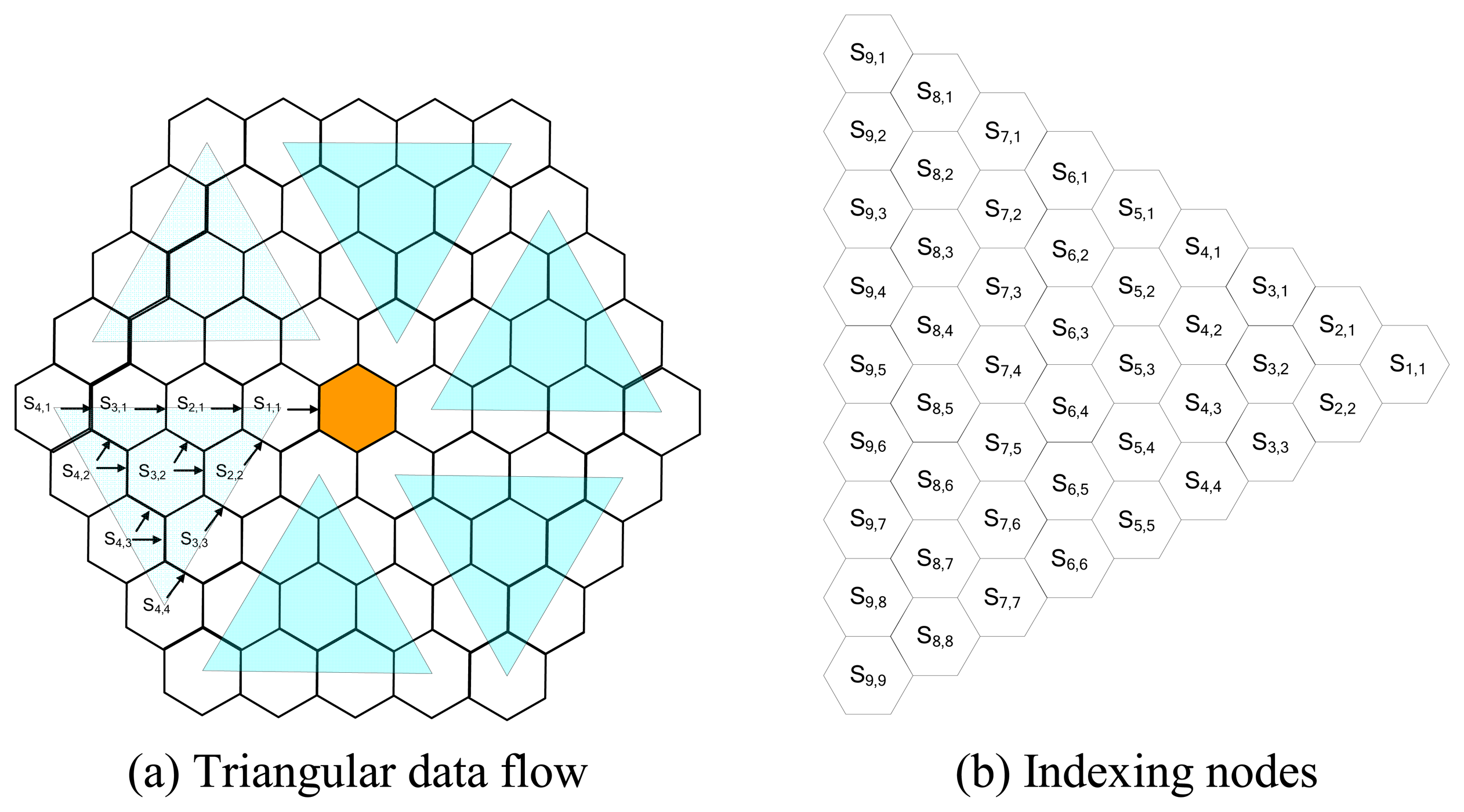
Data acquisition model defines how the data will be accumulated by the cluster head. For this purpose, we divide each -hexagonal- cluster into six triangular regions as depicted in Figure 4(a). Sensor nodes are marked with two subscripts. The first index represents the tier number, which starts with 1 for the innermost tier, and increases as it diverges outwards. The second index represents the sequence of the node in that tier, starts with 1, and increases counter clockwise. S2,3 for example, denotes the sensor node in the 2nd tier, 3rd node counter clockwise from the edge.
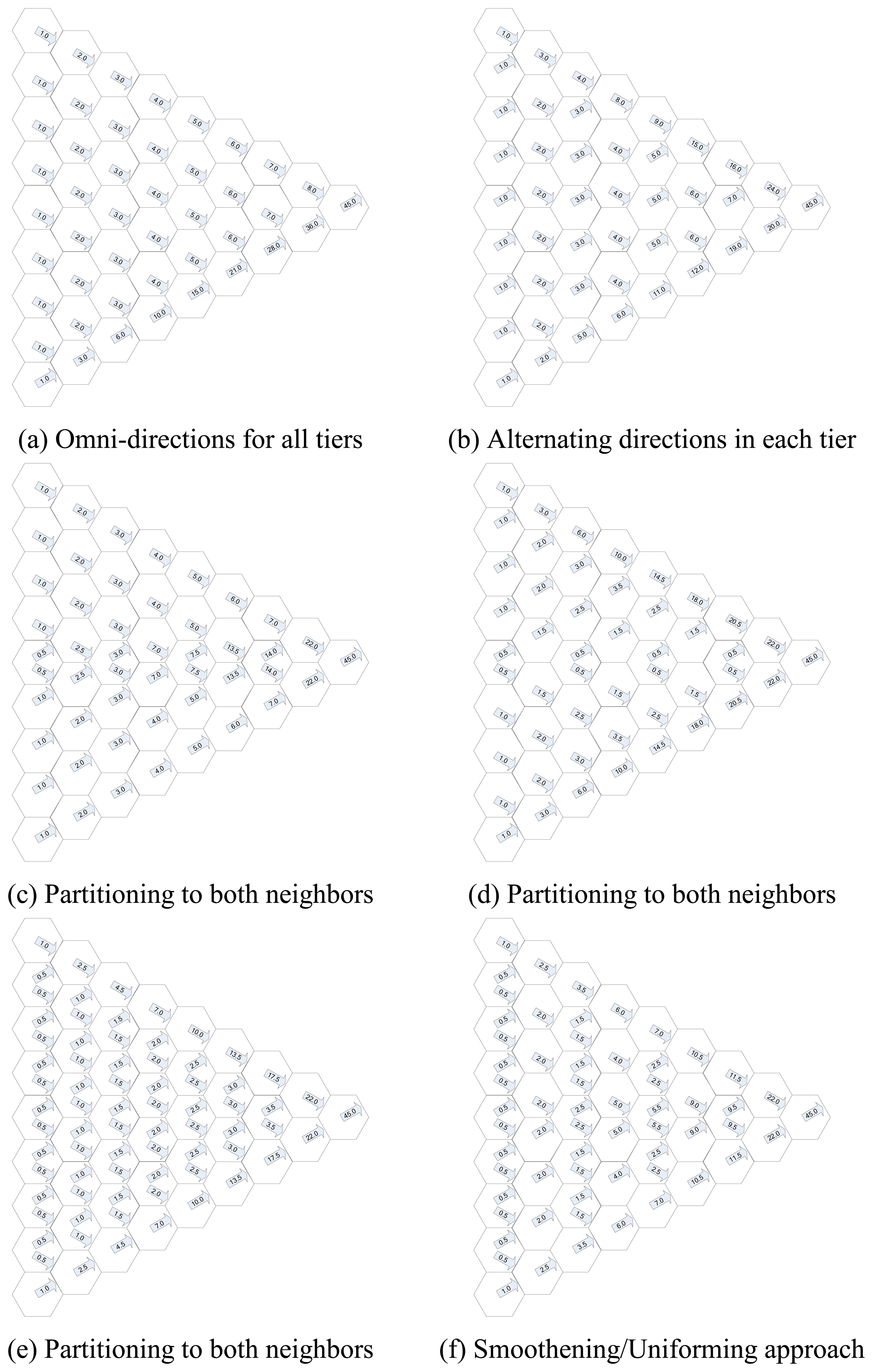
Please remember that FHSM assures existence of a node in the inner tier to send data for any node; otherwise current node needs to slide to fill in the hole. Each sensor node transmits its message to the node in the inner tier and in the same triangle. Since the messages are carried inwards, each message is eventually transferred to the cluster head by the node in the 1st tier. When we look at Figure 4(b), we can see that sensor nodes on either edges of the triangle { Si,j | ( j = 1 ) or ( j = i ) } have only one option, and they send their messages to the sensor nodes on the same edge, those are in the inner tier. Si,1 sends its message to Si-1,1 and Si,i sends its message to Si-1,i-1. There is a vague situation for the internal nodes, though. Internal nodes { Si,j | ( j ≠ 1 ) and ( j ≠ i ) } have two options, such that Si,j can send its message to either Si-1,j-1, or Si-1,j. Selecting the appropriate sensor node to transfer the message requires some work. We analyzed the situation in six significant options as listed below.
- (a)
- Internal nodes may send messages to the node in the same inner tier with the same sequence index, such that sensor node Si,j sends message to Si-1,j. Figure 5a shows this case, and we can see that sensor nodes in each tier are equally loaded, except for the nodes in the lower edge, i.e., Si,i for each tier i, which are overloaded. In this case the algorithm is simple and same for each node except the nodes Si,1.
- (b)
- Internal nodes may send to alternating direction in each tier. Figure 5b shows this case, and we can see that Internal sensor nodes in each tier are loaded as the same as the previous example, and sensor nodes in the lower edge now undertake the load of the upper edge in (a), such that upper and lower nodes are -almost- equally loaded among themselves, which are overloaded from the Internal nodes.
- (c)
- Internal nodes in upper half may send to the nodes with the same index, Internal nodes in lower half may send to the node with one less index, immediate nodes may send half of the messages to the node with the same index, and half of the messages send to the node with one less index. Figure 5c shows this case, and we can see that the nodes have smoother load, except the nodes in the innermost tiers, where the nodes in the middle have more load than the others. It seems that the load of the edge nodes in (a) and (b) are shifted to the intermediate nodes in this case.
- (d)
- Internal nodes in upper half may send to the nodes with one less index, Internal nodes in lower half may send to the nodes with the same index, immediate nodes may send half of the messages to the node with the same index, and half of the messages send to the node with one less index. Figure 5d shows this case, and we can see that the edge nodes have overload as similar to the cases (a) and (b).
- (e)
- Internal nodes (Si,j) may send half of the messages to the node with the same index (Si-1,j), and half of the messages to the node with one lower index (Si-1,j-1). Figure 5e shows this case, and we can see that the Internal nodes in each tier are loaded exactly equal as in both previous examples, but the nodes in both sides in each tier are loaded exactly same, in the contrary with previous examples.
- (f)
- Internal nodes in tiers with odd number of nodes may send half of the messages to the node with the same index, and half of the messages may send to the node with one less index. Internal nodes in upper half in tiers with even number of nodes send to the node with the same index, and half of the messages to the node with one lower index. Figure 5f shows this case, and we can see that the edge nodes have still overload in the tiers close to the cluster head, but in the other tiers loads are well diverged.
We compared number of message loads of nodes in each tier, in order to argue on the choices and choose the best one. We want to remind that our assumptions at the beginning of this section is valid; hence every node generates a message of its own in each cycle, and sends those messages to the cluster head via neighbor nodes. According to this assumption, number of messages those are sent by the nodes in tier 9 in one cycle is 9, since each node transfer its own (1 by each node) message. Tier 8 nodes send their own (totally 8) messages plus messages sent by the node in the tier 9. Hence, totally 17 messages are sent by the tier 8 sensor nodes. Number of total messages sent by the sensor nodes in other tiers are calculated similarly, and shown in Table 1. It also shows average number of messages per each sensor node in that tier.
It is better if all nodes in each tier transfer equal amount of messages to the inner tier because of equal energy consumption eases uniformity in applying algorithms. Hence, we want to equalize number of messages transferred among sensor nodes in each tier as much as possible. For this purpose, we prepared Table 2 that shows standard deviations of the sensor node loads from the average in that tier. The letters in the first column refers to the order of the figure in Figure 5. Hence, data in row a refers to Figure 5(a), for example. The sum of the deviations in each tier is given on the last column. We see that the choice (f) is the best among all, since the sensor nodes in each tier has the lowest total deviations in that option. As a matter of fact, sensor nodes in each tier have lowest variation from other options, not just in the total.
3f. Energy Model: Relocation based on power consumption trends of clusters
Energy level of sensor nodes are digitized by the numbers [0..999] where 999 represents maximum possible initial energy level of any sensor node, and 0 represents the exhausted battery case, under which sensor can not neither sense or communicate, nor relocate.
Our model consists of a clock-driven network, and hence each sensor node sends a periodic message to the cluster head, in T period with the format depicted in Table 3. The sensor nodes also send their energy level information in every ( x * T ) period to the cluster head, where x is some predetermined value. Increasing, or decreasing x is a design issue, and will change the amount of traffic within the network.
After receiving Node Status Reports from each node within the cluster, cluster head calculates total amount of energy of all (n) nodes within the cluster with the summation as in Equation (2), and sends total remaining energy level of the cluster to the sink using Cluster Status Report, which is depicted in Table 4.
When any one of the Number of missing nodes in any cell or Number of cells under critical energy level values are not zero, related relocation activity needs to be planned in the next immediate period. The sink considers the values given with the Cluster Status Reports together with the power consumption rate, pcr of each cluster that the sink calculates, to analyze the need of clusters for relocation. It also checks the availability of clusters for relocating excess nodes to other clusters. It then prepares Sink Migration Instruction as depicted in Table 5, and sends them to the relevant cluster heads. Donor Node ID is node which is expected to relocate to fill the Deprived Cell which creates a hole.
When the Donor Cluster receives the Sink Migration Instruction, it sends corresponding Cluster Migration Instruction to the node(s) within that cluster as depicted in Table 6.
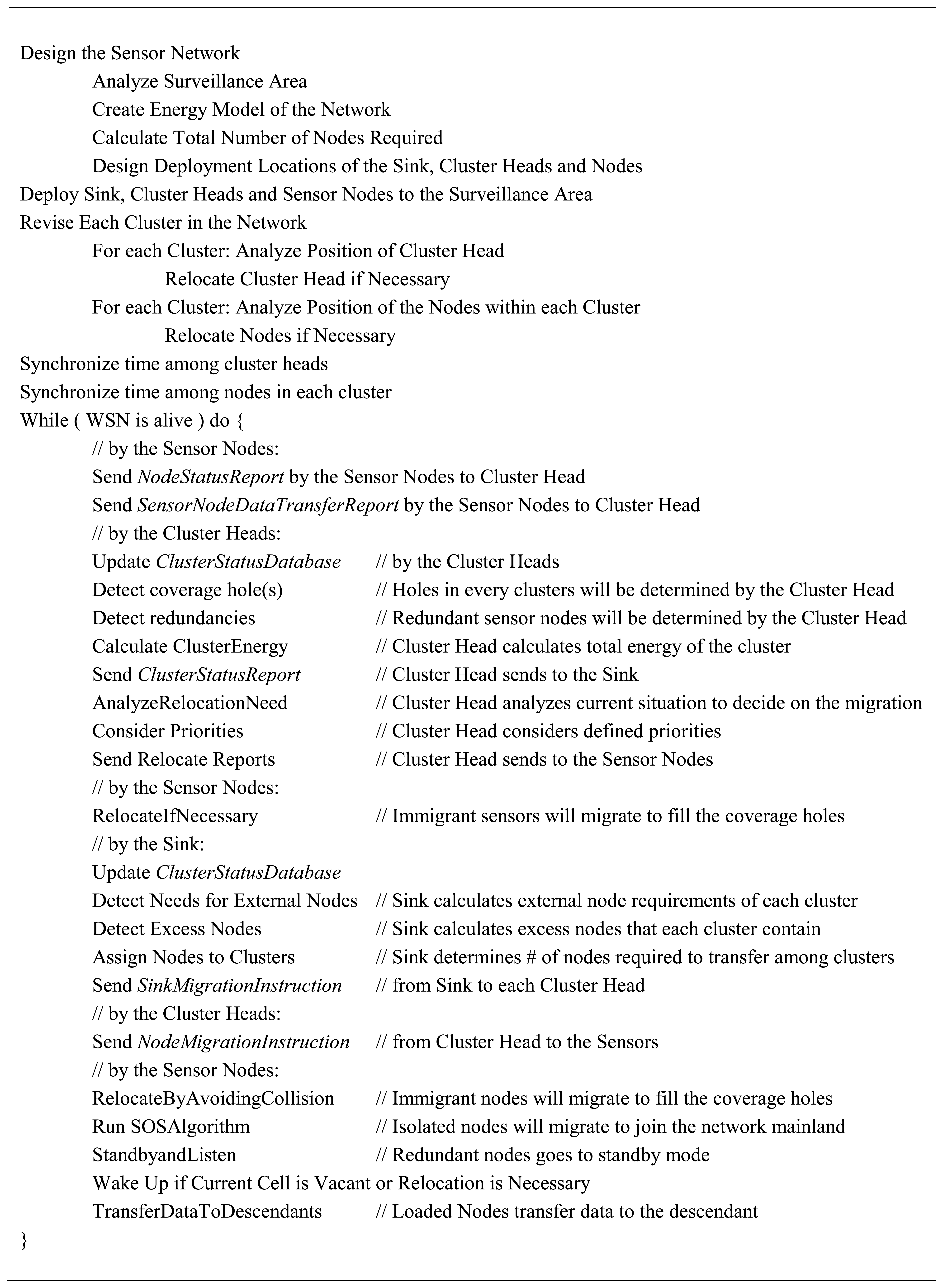
3g. MaxNetLife Algorithm
We depict MaxNetLife algorithm in Figure 6.
3h. Energy Model: Relocation based on power consumption trends of clusters (cont.)
There exists a preemptive part of our algorithm. This part handles the future / estimated need of sensor nodes of all clusters within the network. Sink examines total remaining energy of clusters as it gets the periodic Cluster Status Reports from the clusters. It analyzes energy consumption rate over time, and tries to predict future node relocation need before it actually happens. As it also knows number of redundant sensor nodes in neighbor clusters and knows expected arrival time of redundant sensor nodes from those clusters, it informs the cluster with excess number of sensor nodes to send required number of sensor nodes to the cluster before the node actually die. Therefore the sensor nodes will be in the proper position just before the coverage hole is formed. And migration phase will take only a small amount of time, as we defined above.
Each predecessor sensor node tries to transfer its data to the successor node before it dies. If the successor node arrive the target cell before the predecessor node dies, predecessor node transfers all of its data using the format depicted in Table 7. If it dies before, it tries to send the data to the safe node, which is defined by the cluster head, by using the same format.
4. Performance Evaluations
We analyze various parameters related to mobility of sensor nodes in order to see their affects on MaxNetLife algorithm. We designed and implemented a new simulation environment, called MobilSim, to use in performance evaluation. MobilSim is an object-oriented simulation environment implemented using Java programming language.
4a. Performance metrics & Factoring Parameters
We use hexagonal grid deployment and addressing thru the simulations. The Surveillance area is composed of clusters, and each hexagonal cluster contains either 60 or 220 cells, depending on the model which will be mentioned in the corresponding part below. Nodes are placed deterministically, and are located in the center of the hexagonal cell, so that it can cover whole cell using the embedded sensor. Each sensor node has also enough transmitting range capacity, so that it can transmit its data to the sensor node in the inner tier as well as other neighbor cells.
A very important parameter in the model is power consumption by the sensing, transmission, processing, and relocation activities. There are various studies about power consumption of sensor nodes in the literature, and we select values close to those used in [23]. The energy consumption values used in the simulation are given in Table 8.
The cluster head is located in the middle of the cluster. We model clock-driven networks, and hence every node generates one data packet in each cycle. We model both mobile and immobile networks throughout the simulation, and compare their performances. When a sensor node is to send a data to its neighbor cell, and all nodes are dead in that cell, a node from the outer node relocates to that cell in mobile networks. The mobile node can send its data after relocation is realized and hole is disappeared. In immobile network the hole stays forever, in which case the gap may prevent data being transmitted to the cluster head. The simulation ends when no sensor node remains alive within the clusters, as well as within the network. Networks in all models aims to maximize the amount of total collected information from the surveillance area before the death of the sensor network by increasing cumulative connected coverage of the network as described above sections.
We use two different deployment strategies in our simulations. The first strategy, namely Uniform deployment includes deploying equal number of nodes to each cell. Heuristic deployment, in the contrary, includes deploying more sensor nodes to the cells closer to the cluster head, as described in section 3c.
We used two different network types in the simulations. In immobile network, nodes are not mobile; hence they can not relocate to fill in the holes. In the contrary, nodes relocate to fill the hole in mobile network; according to the MaxNetLife algorithm.
4b. Simulation Results
We created various simulation models to measure the affects of changing relocation cost to be between { 0 … 1,000 }, mobility capability of sensor nodes as { mobile, immobile }, deployment type as { uniform, heuristic }, node density in each cell as { 1 … 50 }, and time; in order to see their affects on the amount of Cumulative Data Transferred to the Cluster head before the death of the network, Number of Alive Cells at Different Times, and Cumulative Connected Coverage of the network.
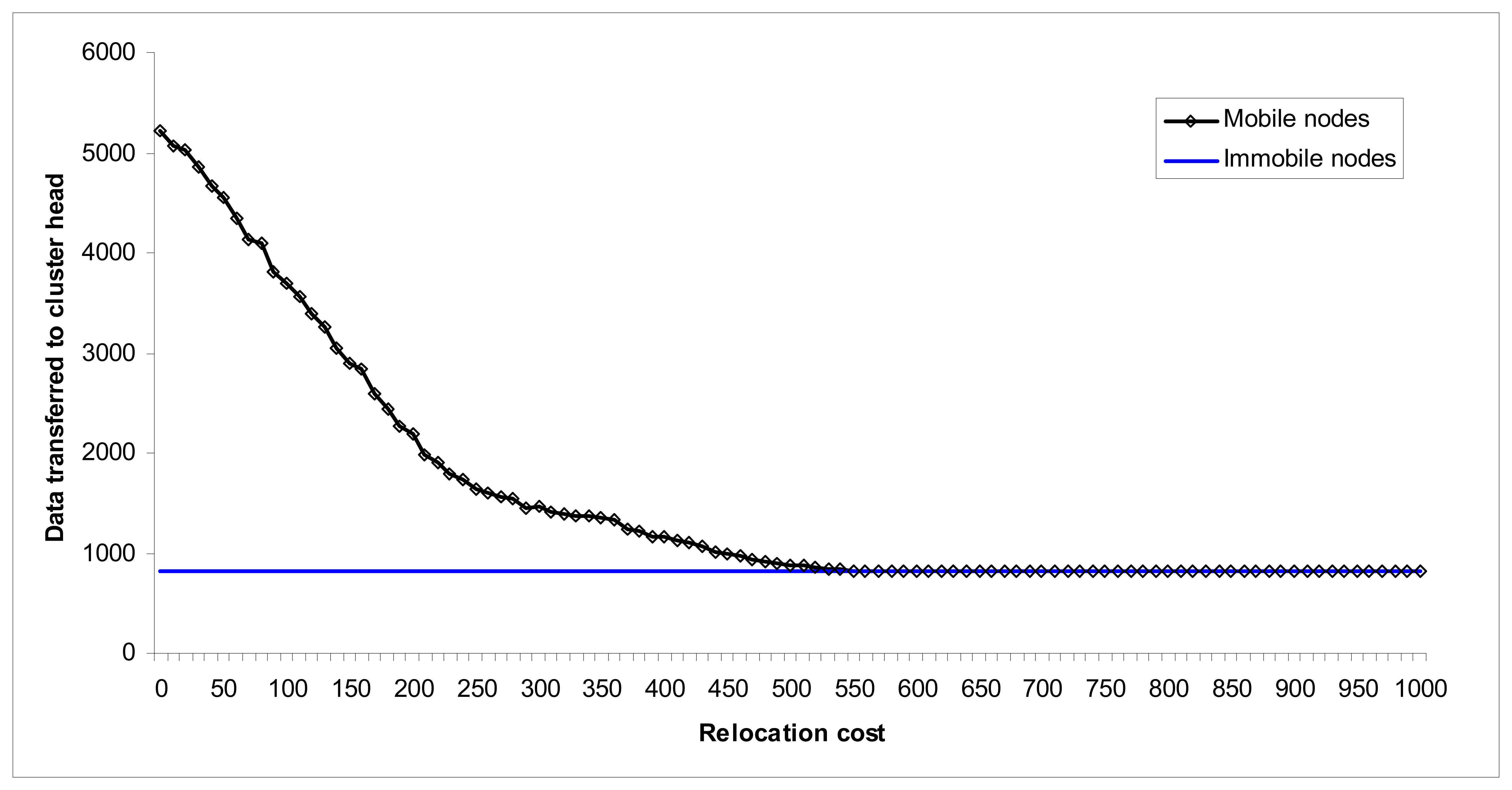
Simulation Model – 1: Effect of relocation cost to transferred data
In this model, we want to measure the affect of relocation cost for mobile sensor nodes on the total amount of data transferred to the cluster head before the network die when uniform deployment is chosen. We also want to compare success of mobile and immobile networks, by counting data transferred to the cluster head in immobile network using the same parameters (except relocation cost). Both mobile and immobile networks have the characteristics shown in Table 9.
In order to measure the effect of mobility, we varied the relocation cost between 1 and 1,000 units. Actually since the initial energy stock of nodes is 1,000 units, only energy consumption < 100 seems reasonable, but we included a wide range anyway.
Figure 7 shows the amount of data packets those arrived to the cluster head before the network dies, i.e. no living node remains. Immobile network generates same amount of (823) data packets independent from the relocation cost, since relocation cost is irrelevant for immobile nodes. In mobile network, total arrived packets are very high for low relocation costs (4559 when relocation cost equals 50, for example) and decreases as relocation cost increases until it is equal to 560 units. Mobile and immobile networks perform equal if relocation cost is higher than 560. Beware of the fact that 560 is more than half of the total initial energy capacity (1,000) of a node, which is not a practical value. For a relatively low relocation cost, mobile network seems to be a very good choice.
Arguments may increase about the reason for mobile network generating more, or at least equal number of data for all values of relocation cost when compared to immobile network. The answer lies in the fact that mobile nodes choose not to relocate if high amount of energy will be consumed. Hence, especially when the relocation cost is very high (like 400-500), most of the sensor nodes does not relocate, hence they perform at least as good as an immobile node. But, even with that high relocation cost, some nodes (especially nodes in the outer tiers) those still include enough remaining energy just relocates to the neighbor cell which increases productivity of mobile network against immobile network alternative.
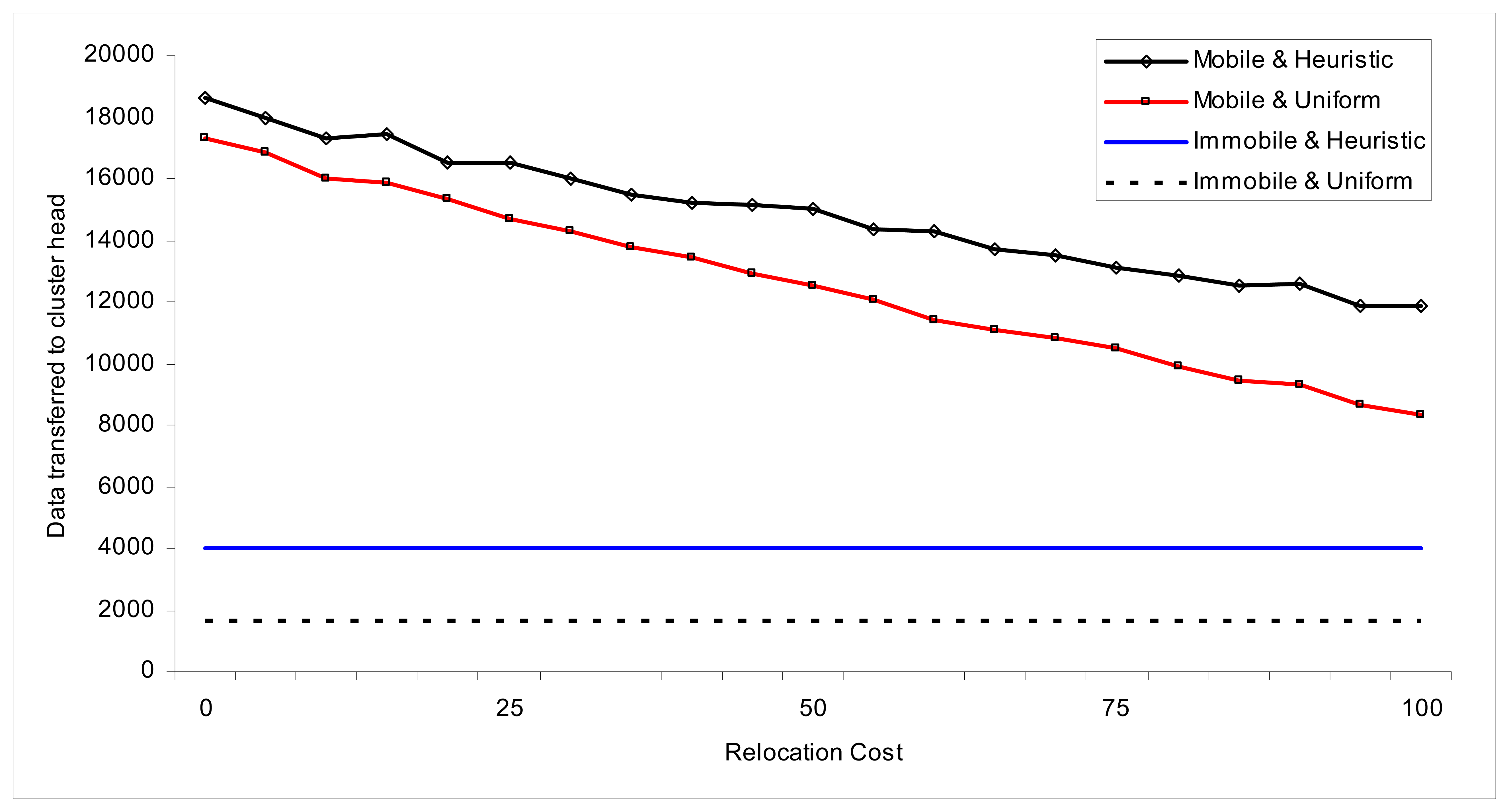
Simulation Model – 2: Effect of deployment type to transferred data
We want to measure the affect of the deployment types together with the mobility. Hence, uniform and heuristic deployments are tested against relocation cost. To see this, we re-created the previous model, by using 220 cells per cluster instead of 60, and 2 nodes per cell, instead of 1, which adds up to 220*2=440 total number of nodes within each cluster. We again measured data transferred to the cluster head until death of the network.
Heuristic network transfers 4032 packets, where uniform network transfers only 1612 in immobile network. In mobile network, heuristic network creates 14,919 where uniform deployment creates only 12,533 packets when relocation cost equals 50.
Figure 8 has two important results. Heuristic deployment creates better results in both mobile and immobile deployment. Heuristic and mobile network using MaxNetLife algorithm outperforms all other options.
Simulation Model – 3: Effect of node density to transferred data
In this model, we measure the effect of node density (number of nodes per cell) to the total number of data transferred to the cluster head before network dies. We simulated both mobile and immobile networks as well as uniform and heuristic deployments, and depicted the results together in Figure 9. Each cluster consists of 60 cells, and node density is varied between 1 and 50. Relocation cost is kept constant (50 units) throughout the simulation.
As we see from Figure 9, number of arrived data packets is always more in mobile network than immobile network for every node density option. We also see from the figure, that heuristic deployment results in higher total number of packets than uniform deployment, a similar result with the previous model. We also conclude that number of data packets is linearly proportional with the node density for both network choices. The result shows that MaxNetLife algorithm is scalable with respect to the node density.
Simulation Model – 4: Effect of cell density to transferred data
In this model, we measure the effect of number of nodes by varying size of the clusters. We varied cluster size between 60 and 220, and also nodes per cell between 1 and 50. Relocation cost is kept constant with 50 units throughout the simulation. We simulated mobile networks using uniform deployment in model.
As we easily see from Figure 10, number of arrived data packets is linearly proportional with cluster size, which is an expected result. The data arrived to the cluster head seemed almost linearly proportional to the cluster size too. The result shows that MaxNetLife algorithm is scalable with respect to the cell density.
Simulation Model – 5: Comparing number of alive cells when Heuristic and Uniform deployment in Mobile vs. Immobile Network are used
A very important indication about the success of an algorithm is number of living cells after a certain period. We already know that higher number of living cells contribute increase in cumulative connected coverage, which is a very important indicator for wireless sensor networks. We try to measure number of living cells as time passes. In this model, number of cells in each cluster is 220; number of deployed nodes to each cell is 2. We included both heuristic as wall as uniform deployment options to see a comprehensive result. Relocation cost is kept constant with 50 units throughout the simulation.
Figure 11 shows that, all of the nodes die within first 15 units of time when equal number of nodes is deployed into each cell in immobile network, and within the first 35 units of time when heuristic deployment is used in immobile network. In the contrary, nodes live much longer in immobile network running MaxNetLife algorithm, better in heuristic than uniform deployment.
Simulation Model – 6: Cumulative Connected Coverage when Heuristic and Uniform deployment in Mobile vs. Immobile Network are used
We included the definition of cumulative connected coverage in previous sections, and we will measure its value against running time in this model. We have the same options as in Figure previous model.
Figure 12 shows many important indicators about the success of MaxNetLife algorithm. Immobile network with uniform deployment dies very early. Death of the sensor nodes closer to the cluster head is the main reason for Cc = 220 in uniform immobile network option. Immobile network with heuristic deployment shows a better performance, since the distribution of the sensor nodes are made considering early energy consumption by the closer nodes, but the network still dies early, and Cc = 516. Mobile network using MaxNetLife algorithm outperforms in both deployment types. Mobile network with uniform deployment creates Cc = 1391. Mobile network with heuristic deployment creates the best result by Cc = 1641.
5. Conclusions
We propose a dynamic relocation algorithm called MaxNetLife, which is mainly based on utilizing the remaining power of individual mobile sensor nodes as well as total remaining power of all sensor nodes in clusters within the surveillance area. It also aims to maximize the amount of total collected valuable information from the surveillance area before the death of the sensor network by increasing cumulative connected coverage throughout the sensor network lifetime. A deterministic approach is used to deploy sensor nodes into the sensor field, where Hexagonal Grid positioning is the selected method to address and locate sensor nodes, since it is the best method to maximize the connected coverage with a given amount of sensor nodes. Excess nodes are preemptively migrated to the cells when number of sensor nodes is decreased below a threshold to prevent a possible hole. When early reaction is impossible, master nodes are relocated to the neighboring cells after the hole occurs. The algorithm also includes details of the relocation activities of the sensor nodes. MaxNetLife assures highest possible cumulative connected coverage before sensor network dies; thus this work outperforms all other relocation related algorithms. We also developed an open-source simulation environment, called MobilSim using Java programming language, which we use in simulating our model.
We created various simulation models to measure the affects of relocation cost, mobility capability, deployment type, node density, and time. Results have proven that mobile sensor network using MaxNetLife algorithm outperforms immobile network. MaxNetLife algorithm is also proved to be effective, scalable in cell density in clusters scalable in node density in nodes, and applicable through simulation.
References
- Akyildiz, I.F.; Su, W.; Sankarasubramaniam, S.Y.; Cayirci, E. Wireless Sensor Networks: A Survey. Elsevier Science B.V. Computer Networks 2001, 38, 393–422. [Google Scholar]
- Akyildiz, I.F.; Su, W.; Sankarasubramaniam, S.Y.; Cayirci, E. A survey on sensor networks. IEEE Communications Magazine 2002, 40, 102–114. [Google Scholar]
- Wang, G.; Cao, G.; Porta, T.L.; Zhang, W. Sensor relocation in mobile sensor networks. Proceedings of the IEEE INFOCOM, Miami, FL, USA, March 2005; pp. 2302–2312.
- Meguerdichian, S.; Koushanfar, F.; Potkonjak, M.; Srivastava, M.B. Coverage problems in wireless ad-hoc sensor networks. Proceedings of the IEEE INFOCOM, Anchorage, AK, USA, April 2001; pp. 1380–1387.
- Clouqueur, T.; Phipatanasuphorn, V.; Ramanathan, P.; Saluja, K.K. Sensor Deployment Strategy for Target Detection. Proceedings of the ACM International Workshop Wireless Sensor Networks and Applications, Atlanta, GA, USA, September 2002; pp. 42–48.
- Howard, A.; Matarić, M.; Sukhatme, G. An Incremental Self-Deployment Algorithm for Mobile Sensor Networks. Autonomous Robots, Special Issue on Intelligent Embedded Systems 2002, 13, 113–126. [Google Scholar]
- Nojeong, H.; Varshney, P.K. Energy-efficient deployment of Intelligent Mobile sensor networks. IEEE Transactions on Man and Cybernetics 2005, 35, 78–92. [Google Scholar]
- Wong, T.; Tsuchiya, T.; Kikuno, T. A self-organizing technique for sensor placement in wireless micro-sensor networks. Proceedings of the International Conference on Advanced Information Networking and Applications, Fukuoka, Kyushu, Japan, March 2004; pp. 78–83.
- Wang, G.; Cao, G.; Porta, T.L. A bidding protocol for deploying mobile sensors. Proceedings of the IEEE International Conference on Network Protocols, Atlanta, GA, USA, November 2003; pp. 315–324.
- Wang, G.; Cao, G.; Porta, T.L. Movement-Assisted Sensor Deployment. IEEE Transactions on Mobile Computing 2006, 5, 640–652. [Google Scholar]
- Sekhar, A.; Manoj, B.S.; Siva, C.; Murthy, R. Dynamic Coverage Maintenance Algorithms for Sensor Networks with Limited Mobility. Proceedings of the IEEE International Conference on Pervasive Computing and Communications, Kauai Island, Hawaii, USA, March 2005; pp. 51–60.
- Cayirci, E.; Govindan, R.; Znati, T.; Srivastava, M.B. Wireless sensor networks. Computer Networks 2003, 43, 417–419. [Google Scholar]
- Iqbal, M.M.; Gondal, I.; Dooley, L. Dynamic symmetrical topology models for pervasive sensor networks. Proceedings of the International Multitopic Conference, Lahore, Pakistan, December 2004; pp. 466–472.
- Yunhuai, L.; Ngan, H.; Lionel, M.N. Power-aware Node Deployment in Wireless Sensor Networks. Proceedings of the IEEE International Conference on Sensor Networks, Ubiquitous, and Trustworthy Computing, Taichung, Taiwan, June 2006; pp. 128–135.
- Wang, X.; Xing, G.; Zhang, Y.; Lu, C.; Pless, R.; Gill, C. Integrated Coverage and Connectivity Configuration in Wireless Sensor Networks. Proceedings of the ACM SenSys, Los Angeles, CA, USA, November 2003; pp. 28–39.
- Mhatre, V.P.; Rosenberg, C.; Kofman, D.; Mazumdar, R.; Shroff, N. A minimum cost heterogeneous sensor network with a lifetime constraint. IEEE Transactions on Mobile Computing 2005, 4, 4–15. [Google Scholar]
- Liu, S.C. A Lifetime-Extending Deployment Strategy for Multi-Hop Wireless Sensor Networks. Proceedings of the Annual Communication Networks and Services Research Conference, Moncton, New Brunswick, Canada, May 2006; pp. 53–60.
- Cayirci, E.; Coplu, T. SENDROM: Sensor networks for disaster relief operations management. Wireless Networks 2007, 13, 409–423. [Google Scholar]
- Cayirci, E. Data aggregation and dilution by modulus addressing in wireless sensor networks. IEEE Communications Letters 2003, 7, 355–357. [Google Scholar]
- Pei, G.; Gerla, M.; Hong, X.; Chiang, C. A wireless hierarchical routing protocol with group mobility. Proceedings of the IEEE Wireless Communications and Networking Conference, New Orleans, LA, USA, September 1999; pp. 1538–1542.
- Cerpa, A.; Estrin, D. ASCENT: adaptive self-configuring sensor networks topologies. IEEE Transactions on Mobile Computing 2004, 3, 272–285. [Google Scholar]
- Somasundara, A.; Kansal, A.; Jea, D.; Estrin, D.; Srivastava, M.B. Controllably Mobile Infrastructure for Low Energy Embedded Networks. IEEE Transactions on Mobile Computing 2006, 5, 958–973. [Google Scholar]
- Dantu, K.; Rahimi, M.; Shah, H.; Babel, S.; Dhariwal, A.; Sukhatme, G.S. Robomote: enabling mobility in sensor networks. Proceedings of the International Symposium on Information Processing in Sensor Networks, Los Angeles, CA, USA, April 2005; pp. 404–409.
Figure 1.
Cluster head placement alternatives.

Figure 2.
Hexagonal cluster formation.

Figure 3.
Data flow among hexagonal grid cells.

Figure 4.
Data flow from sensor nodes to the cluster head.

Figure 5.
Data flow among from sensor nodes to the cluster head.

Figure 6.
Sensor Field Design and Relocation Algorithm

Figure 7.
Effect of relocation cost to number of data arrived to the cluster head.

Figure 8.
Effect of relocation cost to number of data arrived to the cluster head (uniform deployment).
Figure 8.
Effect of relocation cost to number of data arrived to the cluster head (uniform deployment).

Figure 9.
Effect of node density to number of data arrived to the cluster head.

Figure 10.
Effect of node density to number of data arrived to the cluster head.

Figure 11.
Comparing number of alive cells in heuristic deployment with mobile nodes.

Figure 12.
Cumulative Connected Coverage


| Tier | |||||||||
|---|---|---|---|---|---|---|---|---|---|
| 9 | 8 | 7 | 6 | 5 | 4 | 3 | 2 | 1 | |
| Total messages in the tier | 9.00 | 17.00 | 24.00 | 30.00 | 35.00 | 39.00 | 42.00 | 44.00 | 45.00 |
| Average messages per node | 1.00 | 2.13 | 3.43 | 5.00 | 7.00 | 9.75 | 14.00 | 22.00 | 45.00 |
| Tier | ||||||||||
|---|---|---|---|---|---|---|---|---|---|---|
| 9 | 8 | 7 | 6 | 5 | 4 | 3 | 2 | 1 | sum | |
| a | 0.00 | 0.35 | 1.13 | 2.45 | 4.47 | 7.50 | 12.12 | 19.80 | 0.00 | 47.83 |
| b | 0.00 | 0.35 | 0.79 | 1.67 | 2.83 | 4.50 | 6.24 | 2.83 | 0.00 | 19.22 |
| c | 0.00 | 0.23 | 1.13 | 1.55 | 4.47 | 4.33 | 12.12 | 0.00 | 0.00 | 23.84 |
| d | 0.00 | 0.58 | 1.88 | 3.97 | 6.87 | 9.53 | 11.26 | 0.00 | 0.00 | 34.10 |
| e | 0.00 | 0.23 | 0.73 | 1.55 | 2.74 | 4.33 | 6.06 | 0.00 | 0.00 | 15.64 |
| f | 0.00 | 0.23 | 0.73 | 0.89 | 2.45 | 0.87 | 4.33 | 0.00 | 0.00 | 9.50 |
| Field Name | Content |
|---|---|
| Node ID | Node id of the node |
| Tier | The tier of the sensor node |
| Energy | Current energy level of the node |
| Position in the Tier | The index of the sensor node in that tier |
| Current Status | Shows information about current status of the sensor node among {master, extra, excess, relocating, dead} |
| Safe Node | Node Id of the node which stores the data of a dead sensor node. This data will be transferred to the relocated node after it arrives to the cell |
| Data | Data content of the node |
| Cluster ID | number of cells within cluster | number of nodes within cluster |
| Total energy of cluster | number of missing nodes in any cell | number of cells under critical energy level |
| Donor Cluster ID | Donor Node ID | Deprived Cluster ID | Deprived Cell |
| Donor Node ID | Deprived Cluster ID | Deprived Cell |
| Node ID | Cell ID | Data Type1 | Data1 | Data Type2 | Data2 | … |
| Metric | Value (units) |
|---|---|
| Energy stock of each node | 1.000 |
| Energy consumption for sending data | 2 |
| Energy consumption for receiving data | 1 |
| Energy consumption for computation | 2 |
| Metric | Value |
|---|---|
| Deployment type | Uniform |
| Number of cells in each cluster | 60 |
| Number of nodes in each cell | 1 |
| Total number of nodes in each cluster | 60 |
© 2008 by MDPI (http://www.mdpi.org). Reproduction is permitted for noncommercial purposes.
Share and Cite
MDPI and ACS Style
Coskun, V. Relocating Sensor Nodes to Maximize Cumulative Connected Coverage in Wireless Sensor Networks. Sensors 2008, 8, 2792-2817. https://doi.org/10.3390/s8042792
AMA Style
Coskun V. Relocating Sensor Nodes to Maximize Cumulative Connected Coverage in Wireless Sensor Networks. Sensors. 2008; 8(4):2792-2817. https://doi.org/10.3390/s8042792
Chicago/Turabian StyleCoskun, Vedat. 2008. "Relocating Sensor Nodes to Maximize Cumulative Connected Coverage in Wireless Sensor Networks" Sensors 8, no. 4: 2792-2817. https://doi.org/10.3390/s8042792