The Landcover Impact on the Aspect/Slope Accuracy Dependence of the SRTM-1 Elevation Data for the Humboldt Range

Abstract
:1. Introduction
2. Methodology
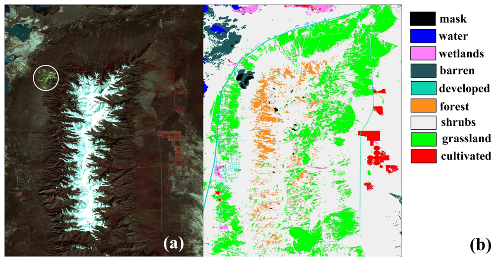
2.1. Study area
2.2 Bare earth DEM, slope and aspect
2.3 SRTM finished DEM
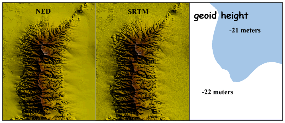
2.4 Orthometric to geodetic height recalculation
2.5 Landcover
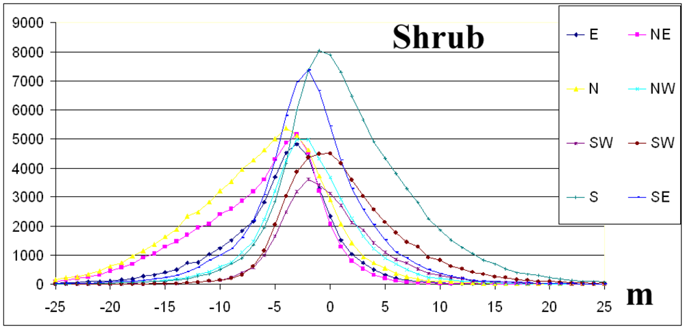
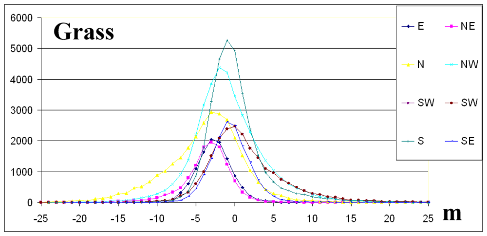
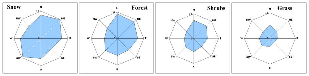
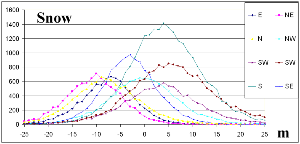
2.6 Directional dependency of elevation differences
2.7 Slope dependency of elevation differences
3. Discussion
4. Conclusions
Acknowledgments
References
- Farr, T.G.; Kobrick, M. Shuttle Radar Topography Mission Produces a Wealth of Data. Amer. Geophys. Union EOS 2000, 81, 583–585. [Google Scholar]
- Slater, J.A.; Garvey, G.; Johnston, C.; Haase, J.; Heady, B.; Kroenung, G.; Little, J. The SRTM Data “Finishing” Process and Products. Photogramm. Eng. Remote Sens. 2006, 72, 237–247. [Google Scholar]
- USGS Seamless Data Distribution System. 2007. http://seamless.usgs.gov/.
- SRTM research-grade data. NASA 's Jet Propulsion Laboratory, 2007. http://www2.jpl.nasa.gov/srtm/.
- Maune, D.; Maitra, J.; McKay, E. Digital Elevation Model Technologies and Applications, the DEM Users Manual; Maune, D., Ed.; American Society for Photogrammetry and Remote Sensing: Bethesda, 2001; Chapter 3; pp. 61–82. [Google Scholar]
- Daniel, C.; Tennant, K. Digital Elevation Model Technologies and Applications, the DEM Users Manual; Maune, D., Ed.; American Society for Photogrammetry and Remote Sensing: Bethesda, 2001; Chapter 12; pp. 395–440. [Google Scholar]
- Finished SRTM data. 2007. http://seamless.usgs.gov/website/seamless/faq/srtm_faq.asp.
- Toutin, T. Impact of Terrain Slope and Aspect on Radargrammetric DEM Accuracy. ISPRS J. Photogramm. Remote Sens. 2002, 57, 228–240. [Google Scholar]
- Miliaresis, G. An Upland Object Based Modeling of the Vertical Accuracy of the SRTM-1 Elevation Dataset. J. Spatial Sci. 2007, 52, 13–29. [Google Scholar]
- Bhang, K.J.; Schwartz, F.; Braun, A. Verification of the Vertical Error in C-Band SRTM DEM Using ICESat and Landsat-7, Otter Tail County, MN. IEEE Trans on Geosci. Remote Sens. 2007, 45, 36–44. [Google Scholar]
- Braun, A.; Fotopoulos, G. Assessment of SRTM, ICESat, and survey control monument elevations in Canada. Photogramm. Eng. Remote Sens. 2007, 73, 1333–1342. [Google Scholar]
- Carabajal, C.C.; Harding, D.J. ICESat validation of SRTM C-band digital elevation models. Geophys. Res. Lett. 2005, 32, L22S01. [Google Scholar] [CrossRef]
- Homer, C.; Huang, C.; Yang, L.; Wylie, B.; Coan, M. Development of a 2001 National Land-cover Database for the United States. Photogramm. Eng. Remote Sens. 2004, 70, 829–840. [Google Scholar]
- Osborn, K.; List, J.; Gesch, D.; Crowe, J.; Merril, G.; Constance, E.; Mauck, J.; Lund, C.; Caruso, V.; Kosovich, J. Digital Elevation Model Technologies and Applications, the DEM Users Manual; Maune, D., Ed.; American Society for Photogrammetry and Remote Sensing: Bethesda, 2001; Chapter 4; pp. 83–120. [Google Scholar]
- Sircombe, K. AGEDispaly: an EXCEL Workbook to Evaluate and Display Univariate Geochronological Data Using Binned Frequency Histograms and Probability Density Distributions. Comput. Geosci. 2004, 30, 21–31. [Google Scholar]
- Clark, W.; Hosking, P. Statistical Methods for Geographers.; John Wiley & Sons: New York, 1986. [Google Scholar]
- Florinsky, I. Derivation of Topographic Variables from a Digital Elevation Models Given by a Spheroidal Trapezoidal Grid. Int. J. Geogr. Info. Sci. 1998, 12, 829–852. [Google Scholar]
- Rodriguez, E.; Morris, C.S.; Belz, J.E. A Global Assessment of the SRTM Performance. Photogramm. Eng. Remote Sens. 2006, 72, 249–261. [Google Scholar]
- Stem, J.E. Use of the NAD/WGS 84 Datum Tag on Mapping Products. National Geodetic Survey, NOAA: Silver Spring, MD, 1995; 72. no. 157. Federal register notice. URL: http://www.ngs.noaa.gov/PUBS_LIB/FedRegister/FRdoc95-19408.pdf.
- Schwarz, C.R. Relation of NAD 83 to WGS 84. Silver Spring, MD: National Geodetic Survey, NOAA, 1989. article 22. p. 249. Professional Paper NOS 2, URL: http://www.mentorsoftwareinc.com/resource/Nad83.htm#Page 249.
- Milbert, D.G.; Smith, D.A. Converting GPS Height into NAVD88 Elevation with the GEOID96 Geoid Height Model. Silver Spring, MD: National Geodetic Survey, NOAA, 1997. http://geodesy.noaa.gov/PUBS_LIB/gislis96.html.
- Lemoine, F.G.; Kenyon, J.K.; Factor, R.G.; Trimmer, N.K.; Pavlis, D.S.; Chinn, C.M.; Cox, S.M.; Klosko, S.B.; Luthcke, M.H.; Torrence, Y.M.; Wang, R.G.; Williamson, E.C.; Pavlis, R.H.; Rapp, T.R.; Olson, P. The Development of the Joint NASA GSFC and the NIMA Geopotential Model EGM96, NASA TP/-1998-206861; NASA Goddard Space Flight Center: Greenbelt, MD, 1999. [Google Scholar]
- Snay, R.A.; Soler, T. Modern terrestrial reference systems, part 3: WGS 84 and ITRS. Prof. Surv. 2000. [Google Scholar]
- NGA. WGS 84 EGM96 15-Minute Geoid Height File and Coefficient File. National Geospatial Agency, Office of GEOINT Sciences, 2007. http://earth-info.nga.mil/GandG/wgs84/gravitymod/egm96/.
- Miliaresis, G.; Paraschou, Ch. Vertical Accuracy of the SRTM DTED Level 1 of Crete. Int. J. Appl. Earth Observ. GeoInfo. 2005, 7, 49–59. [Google Scholar]
- Van Niel, T.G.; McVicar, T.R.; Li, L.T.; Gallant, J.C.; Yang, Q.K. The impact of misregistration on SRTM and DEM image differences. Remote Sens. Environ. 2008. [Google Scholar] [CrossRef]


| ID | Class | Description |
|---|---|---|
| 1 | Water | All areas of open water, generally with less than 25% cover or vegetation or soil |
| 2 | Developed | Includes areas with a mixture of constructed materials and vegetation. These areas most commonly include single-family housing units. |
| 3 | Barren | Barren areas of bedrock. Vegetation accounts for less than 15% of total cover. |
| 4 | Forest | Areas dominated by trees generally greater than 5 meters tall, and greater than 20% of total vegetation cover. |
| 5 | Shrub | Areas dominated by shrubs; less than 5 meters tall with shrub canopy, typically greater than 20% of total vegetation. |
| 6 | Grass | Areas dominated by grammanoid vegetation, generally greater than 80% of total vegetation. |
| 7 | Cultivated | Crop vegetation accounts for greater than 20 percent of total vegetation. Forest or shrub land vegetation or perennial herbaceous vegetation |
| 8 | Wetlands | accounts for greater than 20 percent of vegetative cover and the soil or substrate is periodically saturated or covered with water. |
| Class | Attribute | Aspect direction | ||||||||
|---|---|---|---|---|---|---|---|---|---|---|
| E | NE | N | NW | W | SW | S | SE | All | ||
| Forest | Points | 5726 | 9,130 | 8424 | 1611 | 1046 | 2006 | 7518 | 7382 | 42843 |
| Mean | -7.2 | -9.4 | -9.7 | -3.2 | 0.4 | 2.3 | 0.9 | -3.5 | -5.3 | |
| St.dev. | 6.4 | 5.9 | 6.4 | 6.0 | 6.1 | 7.8 | 7.9 | 6.8 | 8.0 | |
| Skew | -0.2 | -0.3 | 0.0 | 0.2 | 0.0 | 0.4 | -0.2 | -0.4 | 0.2 | |
| RMSE | 9.6 | 11.1 | 11.7 | 6.8 | 6.1 | 8.1 | 8.0 | 7.7 | 9.6 | |
| Grass | Points | 11099 | 11842 | 29463 | 38139 | 22258 | 22258 | 33130 | 15121 | 168189 |
| Mean | -2.7 | -3.6 | -3.8 | -0.8 | 1.5 | 1.5 | 0.1 | -0.5 | -0.9 | |
| St.dev. | 2.5 | 3.3 | 5.3 | 4.7 | 5.1 | 5.1 | 3.8 | 2.7 | 5.0 | |
| Skew | 0.0 | -0.9 | -0.2 | 0.5 | 0.9 | 0.8 | 0.9 | 0.8 | 0.6 | |
| RMSE | 3.6 | 4.9 | 6.5 | 4.8 | 5.3 | 5.3 | 3.8 | 2.8 | 5.1 | |
| Shrub | Points | 42327 | 55901 | 71253 | 44784 | 33061 | 50056 | 93974 | 67236 | 458592 |
| Mean | -4.5 | -6.7 | -6.7 | -1.9 | -0.1 | 1.4 | 1.9 | -1.8 | -2.2 | |
| St.dev. | 5.2 | 6.0 | 6.5 | 4.8 | 4.8 | 5.7 | 6.3 | 5.3 | 6.7 | |
| Skew | -0.4 | -0.6 | -0.3 | 0.1 | 0.6 | 0.9 | 0.7 | 0.2 | 0.0 | |
| RMSE | 6.9 | 9.1 | 9.3 | 5.2 | 4.8 | 5.9 | 6.5 | 5.6 | 7.0 | |
| Snow | Points | 8555 | 9381 | 10419 | 11236 | 10250 | 17632 | 24907 | 12836 | 105216 |
| Mean | -7.5 | -10.5 | -7.7 | -0.3 | 3.5 | 6.3 | 4.5 | -3.1 | -0.3 | |
| St.dev. | 5.9 | 6.3 | 7.5 | 7.9 | 8.8 | 10.0 | 8.1 | 6.0 | 9.9 | |
| Skew | 0.1 | 0.4 | 0.4 | 0.1 | 0.0 | 0.2 | 0.3 | 0.1 | 0.3 | |
| RMSE | 9.5 | 12.3 | 10.8 | 7.9 | 9.5 | 11.9 | 9.2 | 6.7 | 9.9 | |
| Class | Attribute | Slope in degrees | |||||||||
|---|---|---|---|---|---|---|---|---|---|---|---|
| E | NE | N | NW | W | SW | S | SE | All | |||
| Forest | Mean | 18.8 | 22.8 | 29.6 | 21.6 | 16.8 | 21.6 | 28.2 | 22.5 | 24.2 | |
| St.dev. | 6.1 | 7.2 | 8.2 | 7.9 | 8.3 | 9.1 | 9.4 | 7.4 | 8.8 | ||
| Grass | Mean | 4.7 | 7.4 | 17.4 | 12.3 | 9.0 | 10.2 | 8.4 | 5.5 | 10.4 | |
| St.dev. | 3.4 | 7.1 | 11.4 | 9.2 | 7.4 | 8.6 | 8.2 | 4.4 | 9.3 | ||
| Shrub | Mean | 12.0 | 16.2 | 23.1 | 13.7 | 13.3 | 13.1 | 20.8 | 15.4 | 16.9 | |
| St.dev. | 8.1 | 10.2 | 15.5 | 9.9 | 16.5 | 9.5 | 12.4 | 10.5 | 11.8 | ||
| Snow | Mean | 19.7 | 23.8 | 30.1 | 27.1 | 23.3 | 27.2 | 31.4 | 23.4 | 26.7 | |
| St.dev. | 5.1 | 6.6 | 8.5 | 7.5 | 6.7 | 7.1 | 7.4 | 6.4 | 8.0 | ||
| Attributes | E | NE | N | NW | W | SW | S | SE | |||
|---|---|---|---|---|---|---|---|---|---|---|---|
| Forest | b | -4.03 | -5.19 | -3.12 | -4.59 | -4.19 | -5.49 | -6.02 | -6.94 | ||
| a | -0.20 | -0.19 | -0.23 | 0.06 | 0.30 | 0.37 | 0.24 | 0.16 | |||
| a in degrees | -11.5 | -10.7 | -12.8 | 3.5 | 16.6 | 20.2 | 13.5 | 8.9 | |||
| R | 0.55 | 0.96 | 0.96 | 0.42 | 0.60 | 0.94 | 0.96 | 0.81 | |||
| Grass | b | -1.31 | -0.87 | -0.50 | 0.44 | 0.56 | -0.70 | -1.94 | -2.50 | ||
| a | -0.15 | -0.29 | -0.18 | -0.06 | 0.08 | 0.25 | 0.24 | 0.14 | |||
| a in degrees | -8.6 | -16.2 | -10.3 | -3.5 | 4.3 | 14.1 | 13.7 | 7.8 | |||
| R | 0.73 | 0.95 | 0.96 | 0.46 | 0.28 | 0.96 | 0.99 | 0.55 | |||
| Shrubs | b | -2.34 | -1.03 | -0.66 | -0.86 | -1.20 | -2.68 | -2.38 | -2.83 | ||
| a | -0.18 | -0.35 | -0.26 | -0.06 | 0.15 | 0.32 | 0.20 | 0.07 | |||
| a in degrees | -10.3 | -19.4 | -14.5 | -3.3 | 8.7 | 17.5 | 11.4 | 3.8 | |||
| R | 0.82 | 0.99 | 0.99 | 0.71 | 0.71 | 0.99 | 1.00 | 0.82 | |||
| Snow | B | -4.06 | -0.23 | 0.98 | 1.28 | 1.71 | 1.09 | 0.21 | -0.54 | ||
| a | -0.02 | -0.42 | -0.29 | -0.05 | -0.08 | 0.09 | 0.22 | 0.15 | |||
| a in degrees | -1.1 | -22.9 | -16.4 | -3.1 | -4.5 | 5.0 | 12.7 | 8.8 | |||
| R | 0.04 | 0.99 | 0.95 | 0.51 | 0.70 | 0.61 | 0.97 | 0.91 | |||
© 2008 by the authors; licensee Molecular Diversity Preservation International, Basel, Switzerland. This article is an open-access article distributed under the terms and conditions of the CreativeCommons Attribution license ( http://creativecommons.org/licenses/by/3.0/).
Share and Cite
Miliaresis, G.C. The Landcover Impact on the Aspect/Slope Accuracy Dependence of the SRTM-1 Elevation Data for the Humboldt Range. Sensors 2008, 8, 3134-3149. https://doi.org/10.3390/s8053134
Miliaresis GC. The Landcover Impact on the Aspect/Slope Accuracy Dependence of the SRTM-1 Elevation Data for the Humboldt Range. Sensors. 2008; 8(5):3134-3149. https://doi.org/10.3390/s8053134
Chicago/Turabian StyleMiliaresis, George C. 2008. "The Landcover Impact on the Aspect/Slope Accuracy Dependence of the SRTM-1 Elevation Data for the Humboldt Range" Sensors 8, no. 5: 3134-3149. https://doi.org/10.3390/s8053134