Validation and Variation of Upper Layer Thickness in South China Sea from Satellite Altimeter Data

Abstract
:1. Introduction
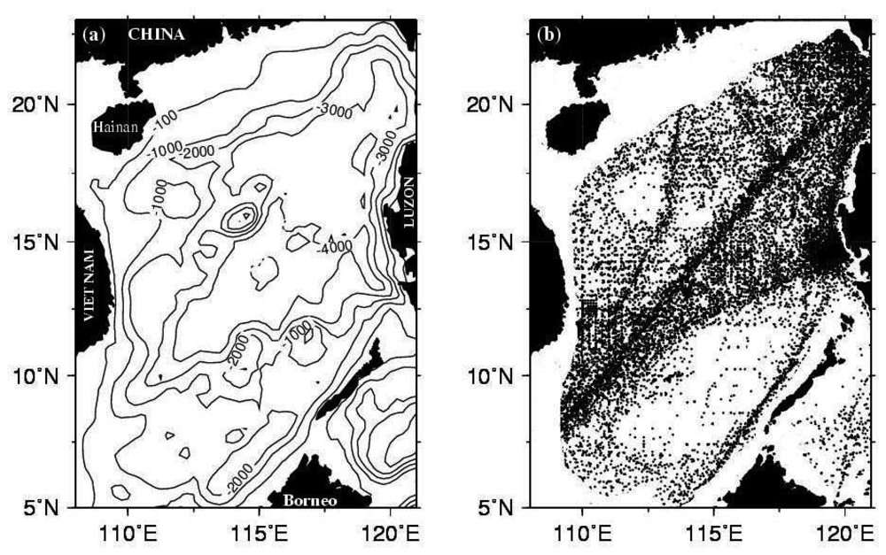
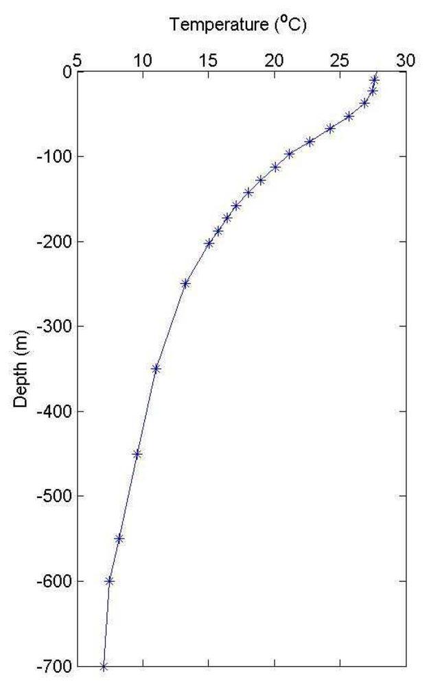
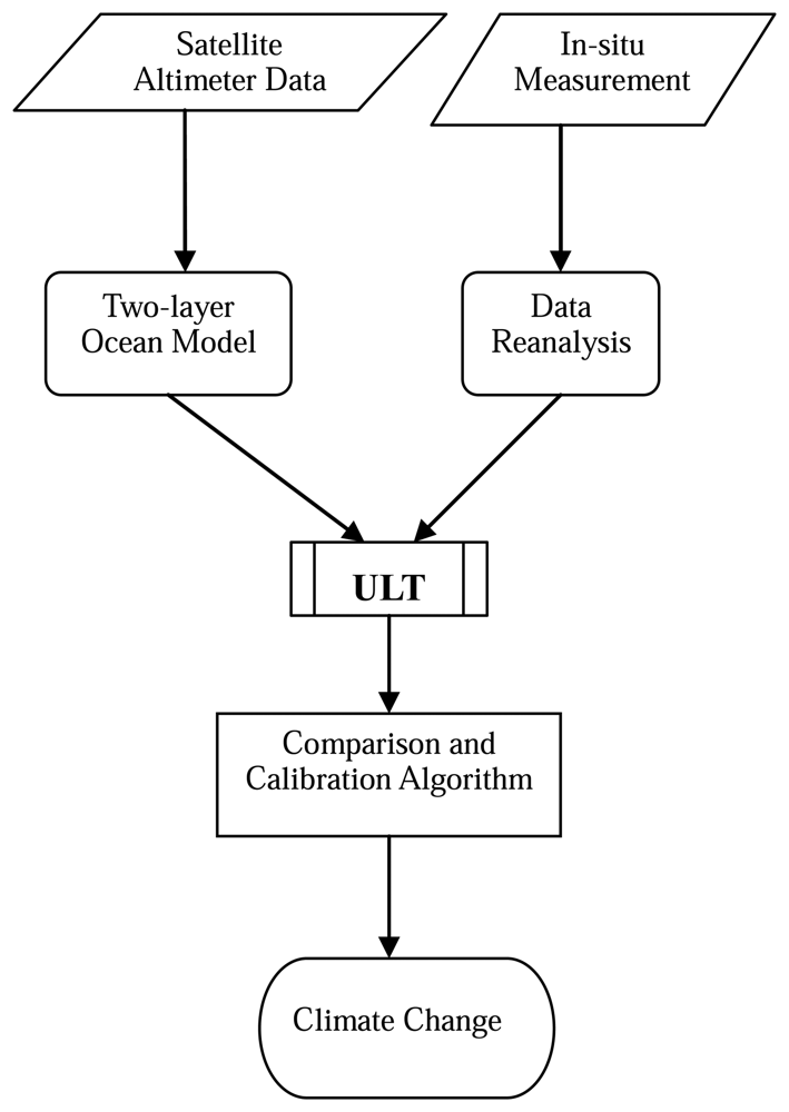
2. Data and Data Processing
3. Two-Layer Reduced Gravity Ocean Model
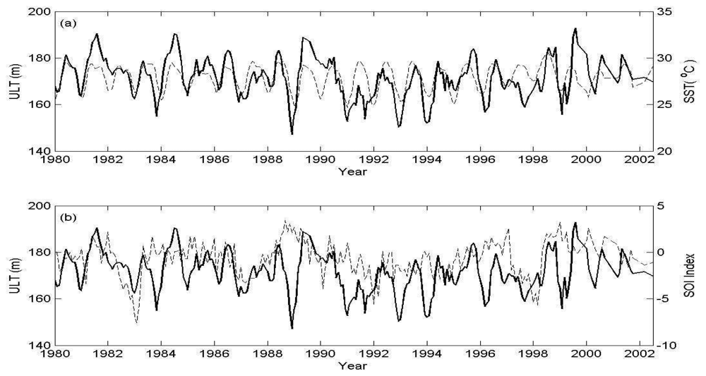
4. Validation
5. Variation
6. Summary
Acknowledgments
References and Notes
- Chao, S.-Y.; Shaw, P.-T.; Wu, S.Y. El Niño modulation of the South China Sea circulation. Prog. Oceanogr. 1996, 38, 51–93. [Google Scholar]
- Chu, P.C.; Lu, S.H.; Chen, Y.C. Wind driven South China Sea deep basin warm-core and cool-core eddies. J. Oceanogr. 1998, 54, 347–360. [Google Scholar]
- Wu, C.-R.; Chang, C.W.J. Interannual variability of the South China Sea in a data assimilation model 2005. Geophys. Res. Letts. 2005, 32. [Google Scholar] [CrossRef]
- Shaw, P.-T.; Chao, S.-Y.; Fu, L. Sea Surface height variation in the South China Sea from satellite altimetry. Oceanol. Acta. 1999, 22, 1–17. [Google Scholar]
- Shay, L.K.; Goni, G.J.; Black, P.G. Effects of a warm oceanic feature on Hurricane Opal. Mon. Wea. Rev. 2000, 128, 1366–1383. [Google Scholar]
- Lau, K.M. South China Sea Monsoon Experiment (SCSMEX) observed from satellite. EOS. Trans. Amer. Geophys. Union 1997, 78, 599–603. [Google Scholar]
- Levitus, S.; Boyer, T.P. World Ocean Atlas 1994 Vol. 4: Temperature; NOAA Atlas NESDIS 4, Natl. Oceanic and Atmos. Admin.: Silver Spring, Maryland, 1994. [Google Scholar]
- Fu, L.-L.; Cheney, R.E. Application of satellite altimeter to ocean circulation studies: 1987-1994. Rev. Geophys. 1995, 33, 212–223. [Google Scholar]
- Goni, G.J.; Kamholz, S.; Garzoli, S.L.; Olson, D.B. Dynamics of the Brazil-Malvinas confluence based on inverted echo sounders and altimetry. J. Geophys. Res. 1996, 101, 16,273–16,289. [Google Scholar]
- Garzoli, S.L.; Goni, G.J.; Mariano, A.J.; Olson, D.B. Monitoring the upper southeastern Atlantic transports using altimeter data. J. Marine Res. 1997, 55, 453–481. [Google Scholar]
- Pun, I.-F.; Lin, I.-I.; Wu, C.-R.; Ko, D.-S.; Liu, W.-T. Validation and Application of Altimetry-Derived Upper Ocean Thermal Structure in the Western North Pacific Ocean for Typhoon-Intensity Forecast. IEEE Trans. Geoscience and Remote Sens. 2007, 45, 1616–1630. [Google Scholar]
- Sainz-Trapaga, S.; Goni, M.G.J.; Sugimoto, T. Identification of the Kuroshio Extension, its Bifurcation and Northern Branch from altimetry and hydrographic data during October 1992 -August 1999: Spatial and temporal variability. Geophys. Res. Letts. 2001, 28, 1759–1762. [Google Scholar]
- Chen, S.-A. Space-time variations of the TOPEX/POSEIDON-derived heat storage anomaly over the Kuroshio upstream regions. Remote Sens. Environ. 2003, 89, 128–137. [Google Scholar]
- White, W.; Tai, C-K. Inferring interannual changes in global upper ocean heat storage from TOPEX altimetry. J. Geophys. Res. 1995, 100, 24,943–24,954. [Google Scholar]
- Gilson, J.; Roemmich, D.; Comuelle, B. Relationship of TOPEX/Poseidon altimetric height to steric height and circulation in the North Pacific. J. Geophys. Res. 1998, 103, 27,947–27,965. [Google Scholar]
- Polito, P.S.; Sato, O.T. Patterns of sea surface height and heat storage associated to intraseasonal Rossby waves in the tropics. J. Geophys. Res. 2003, 108. [Google Scholar] [CrossRef]
- Boyer, T.; Levitus, S. Quality control and processing of historical oceanographic temperature, salinity, and oxygen data.; NOAA Technical Report NESDIS 81: Washington D.C., 1994. [Google Scholar]
- Tapley, B.D.; Watkins, M.M.; Ries, J.C.; Davis, G.W.; Eanes, R.J.; Poole, S.R.; Rim, H.J.; Schutz, B.E.; Shum, C.K.; Nerem, R.S.; Lerch, F.J.; Marshall, J.A.; Klosko, S.M.; Pavlis, N.K.; Williamson, G.G. The joint gravity model 3. J. Geophys. Res. 1996, 101, 28,029–28,049. [Google Scholar]
- Fu, L.L.; Christensen, E.J.; Yamarone, C.A.; Lefebvre, M.; Menard, Y.; Dorrer, M.; Escudier, P. TOPEX/POSEIDON mission overview. J. Geophys. Res. 1994, 99, 24369–24381. [Google Scholar]
- Willis, P.; Haines, B.; Bar-Sever, Y.; Bertiger, W.; Muellerschoen, R.; Kuang, D.; Desai, S. Topex/Jason combined GPS/DORIS orbit determination in the tandem phase. Adv. Space Res. 2003, 31, 1941–1946. [Google Scholar]
- Ho, C.-R.; Zheng, Q.; Soong, Y.-S.; Kuo, N.-J.; Hu, J.-H. Seasonal variability of sea surface height in South China Sea observed with TOPEX/Poseidon altimeter data. J. Geophys. Res. 2000, 105, 13,891–13,990. [Google Scholar]
- Worthington, L.V. The 18° water in the Sargasso Sea. Deep-Sea Res. 1959, 5, 297–305. [Google Scholar]
- Wang, B.; Wu, R.; Lukas, R. Annual adjustment of the thermocline in tropical Pacific Ocean. J. Climate 2000, 13, 596–616. [Google Scholar]
- Grey, S.M.; Haines, K.; Troccoli, A. A Study of Temperature Changes in the Upper North Atlantic: 1950-94. J. Climate 2000, 13, 2697–2711. [Google Scholar]
- Chambers, D.P.; Tapley, B.D.; Stewart, R.H. Long-period ocean heat storage rates and basin-scale fluxes from TOPEX. J. Geophys. Res. 1997, 10525–10533. [Google Scholar]
- Chambers, D.P.; Tapley, B.D.; Stewart, R.H. Measuring heat storage changes in the Equatorial Pacific: A comparison between TOPEX altimetry and Tropical Atmosphere-Ocean buoys. J. Geophys. Res. 1998, 103, 18591–18597. [Google Scholar]
- Soong, Y.-S.; Hu, J.-H.; Ho, C.-R.; Niiler, P.P. Cold core eddy detected in South China Sea. EOS. Trans. Amer. Geophys. Union 1995, 76, 345–347. [Google Scholar]
- Ho, C.-R.; Kuo, N.-J.; Zheng, Q.; Soong, Y.-S. Dynamically active area in the South China Sea detected from TOPEX/Poseidon satellite altimeter data. Remote Sens. Environ. 2000, 71, 320–328. [Google Scholar]
- Qu, T. Upper-layer circulation in South China Sea. J. Phys. Oceanogr. 2000, 30, 1450–1460. [Google Scholar]
- Sato, O.; Polito, P.S.; Liu, W.T. Importance of salinity measurements in heat storage estimation from TOPEX/POSEIDON. Geophys. Res. Lett. 2000, 27, 549–551. [Google Scholar]
- Polito, P.S.; Sato, O.T.; Liu, W.T. Characterization and validation of heat storage variability from TOPEX/POSEIDON at four oceanographic sites. J. Geophys. Res. 2000, 105, 16911–16921. [Google Scholar]
- Gan, J.; Qu, T. Coastal jet separation and associated flow variability in the Southwest South China Sea. Deep-Sea Res. I 2008, 55, 1–19. [Google Scholar]
- Kuo, N.-J.; Zheng, Q.; Ho, C.-R. Satellite observation of upwelling along the western coast of the South China Sea. Remote Sens. Environ. 2000, 74, 462–469. [Google Scholar]
- Kuo, N.-J.; Zheng, Q.; Ho, C.-R. Response of Vietnam coastal upwelling to the 1997-1998 ENSO event observed by multisensor data. Remote Sens. Environ. 2004, 89, 106–115. [Google Scholar]
- Zheng, Z.-W.; Ho, C.-R.; Kuo, N.-J. Mechanism of weakening of west Luzon eddy during La Nina years. Geophys. Res. Lett. 2005, 34. [Google Scholar] [CrossRef]


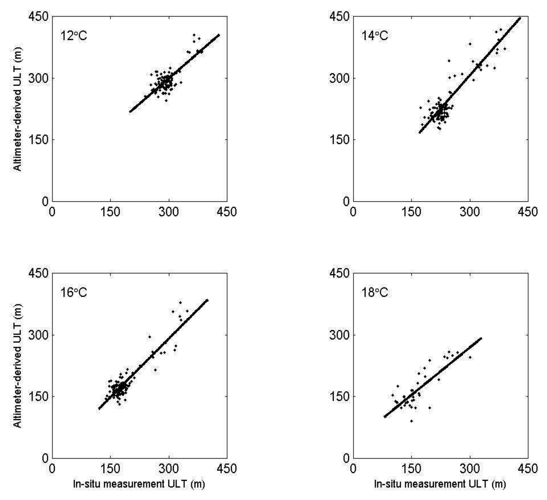
| Temperature of ULT depth (°C) | Correlation coefficient | slop | Intercept (m) |
|---|---|---|---|
| 12 | 0.78 | 0.82 | 53 |
| 14 | 0.90 | 1.07 | -17 |
| 16 | 0.92 | 0.95 | 6 |
| 18 | 0.83 | 0.78 | 38 |
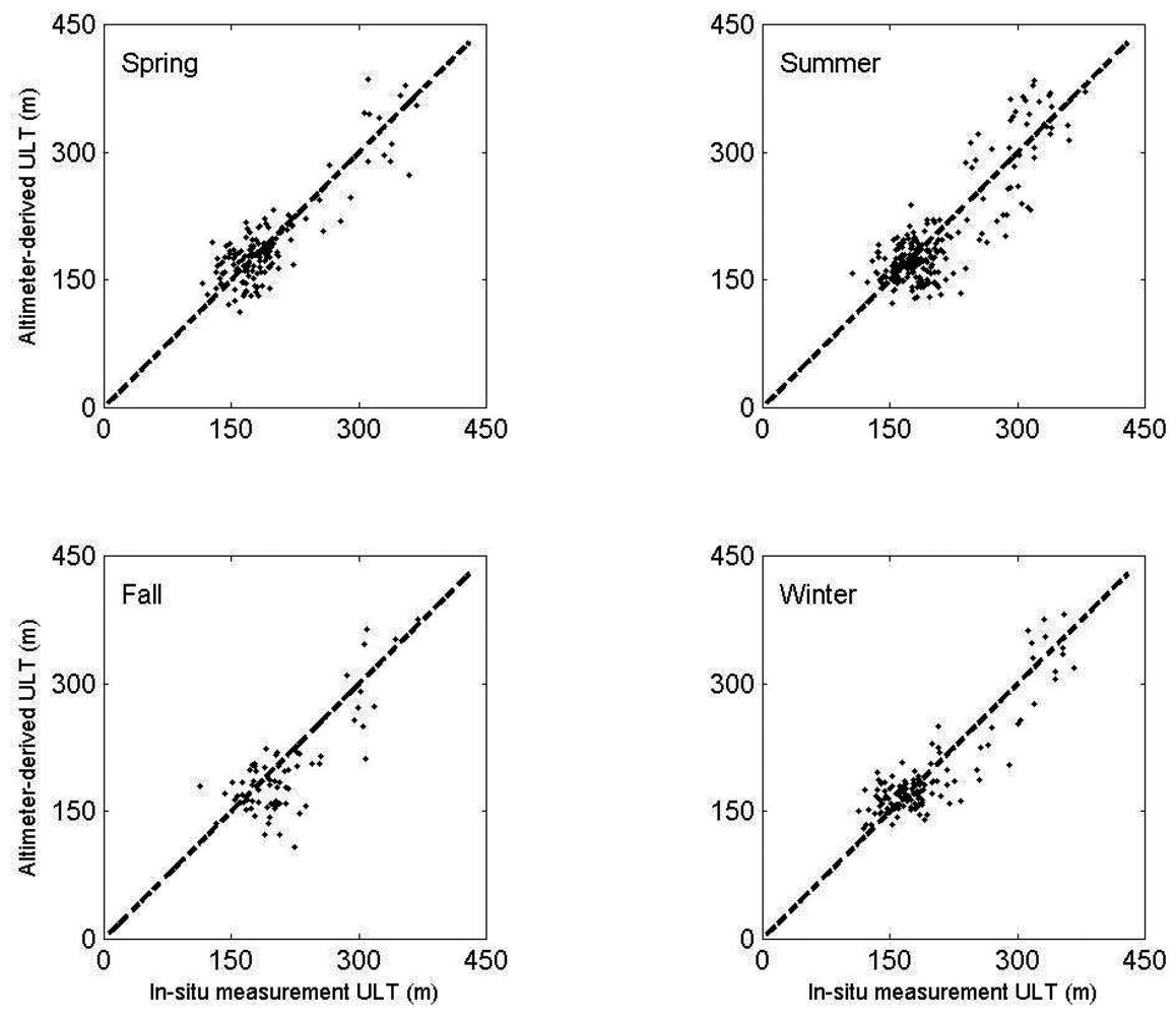
| Season | Correlation coefficient | RMS (m) | MAPE (%) | Bias (m) |
|---|---|---|---|---|
| Spring | 0.88 | 28 | 11 | 1 |
| Summer | 0.85 | 31 | 12 | -3 |
| Fall | 0.79 | 41 | 14 | 10 |
| Winter | 0.90 | 26 | 11 | -3 |
© 2008 by the authors; licensee Molecular Diversity Preservation International, Basel, Switzerland. This article is an open-access article distributed under the terms and conditions of the Creative Commons Attribution license ( http://creativecommons.org/licenses/by/3.0/).
Share and Cite
Lin, C.-Y.; Ho, C.-R.; Zheng, Z.-W.; Kuo, N.-J. Validation and Variation of Upper Layer Thickness in South China Sea from Satellite Altimeter Data. Sensors 2008, 8, 3802-3818. https://doi.org/10.3390/s8063802
Lin C-Y, Ho C-R, Zheng Z-W, Kuo N-J. Validation and Variation of Upper Layer Thickness in South China Sea from Satellite Altimeter Data. Sensors. 2008; 8(6):3802-3818. https://doi.org/10.3390/s8063802
Chicago/Turabian StyleLin, Chun-Yi, Chung-Ru Ho, Zhe-Wen Zheng, and Nan-Jung Kuo. 2008. "Validation and Variation of Upper Layer Thickness in South China Sea from Satellite Altimeter Data" Sensors 8, no. 6: 3802-3818. https://doi.org/10.3390/s8063802