Detecting Aquatic Vegetation Changes in Taihu Lake, China Using Multi-temporal Satellite Imagery

Abstract
:1. Introduction
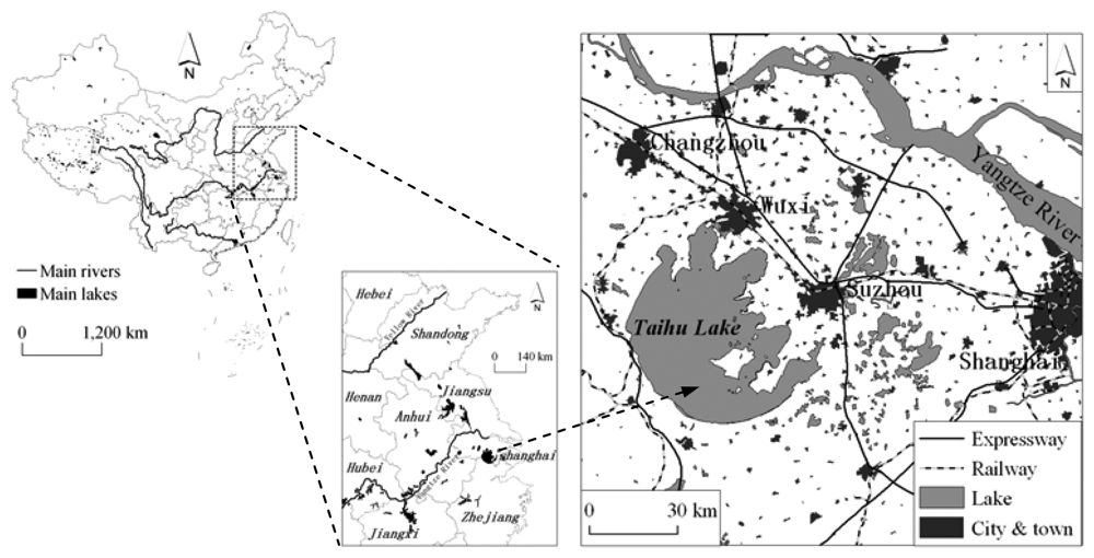
2. Study area
3. Material
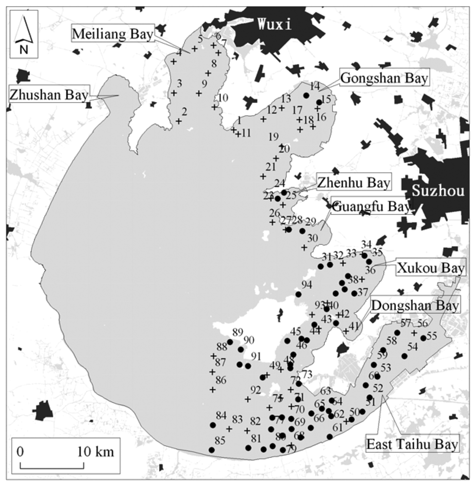
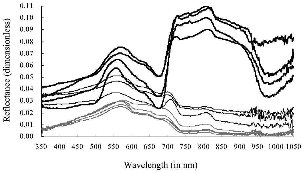
3.1 Field data
3.2 Satellite data
4. Methods
4.1 Image preprocessing
4.2 Image classification
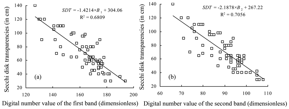
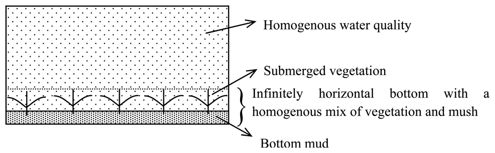
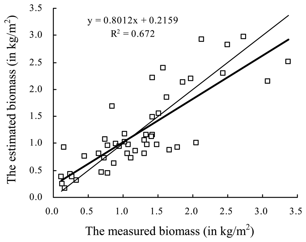
4.3 Biomass estimation
5. Results
5.1 Field investigation
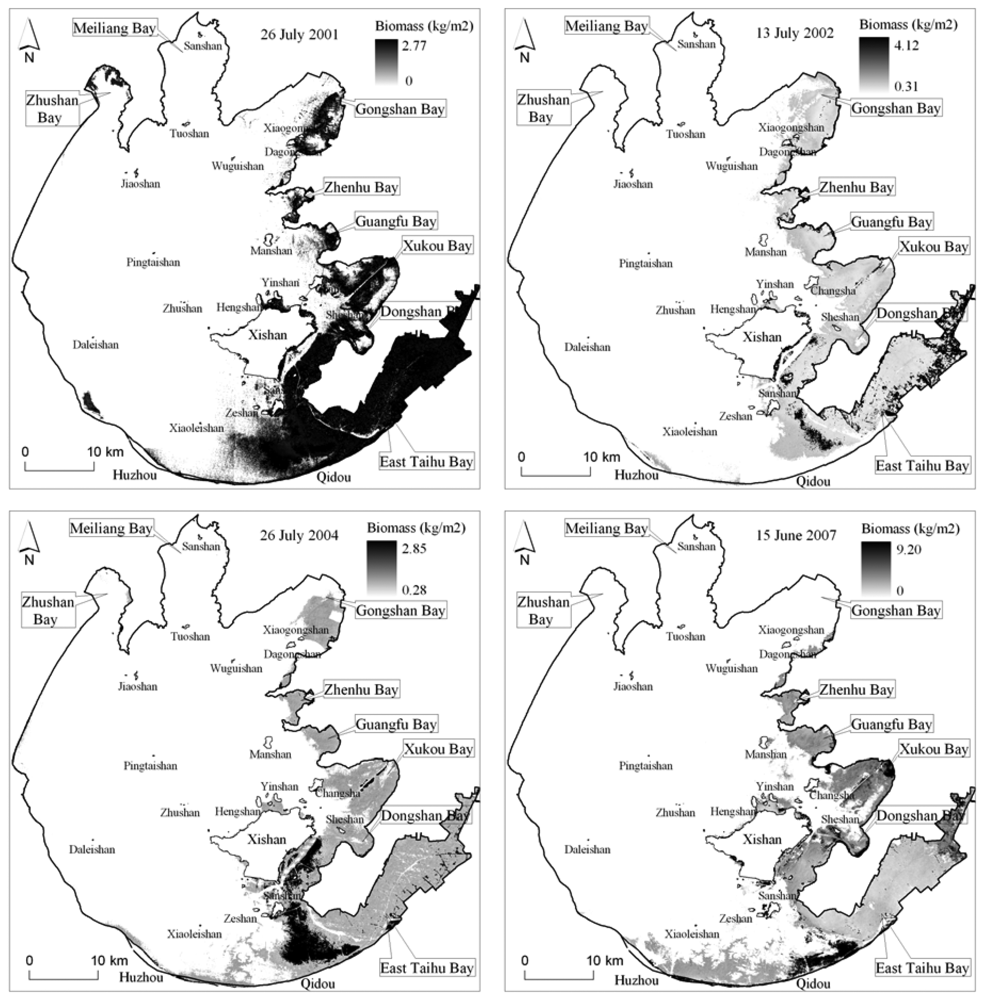
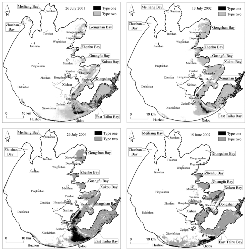
5.1 Remote sensing classification and estimation
6. Discussion
7. Conclusions
Acknowledgments
References and Notes
- Vis, C.; Hudon, C.; Carignan, R. An evaluation of approaches used todetermine the distribution and biomass of emergent and submerged aquatic macrophytes over large spatial scales. Aquat. Bot. 2003, 77, 187–201. [Google Scholar]
- Malthus, T.J.; George, D.G. Airborne remote sensing of macrophytes in Cefni Reservoir, Anglesey, UK. Aquat. Bot. 1997, 58, 317–332. [Google Scholar]
- Marshall, T.R.; Lee, P.F. Mapping aquatic macrophytes through digital image analysis of aerial photographs: an assessment. J. Aquat. Plant Manag. 1994, 32, 61–66. [Google Scholar]
- Penuelas, J.; Gamon, J.A.; Griffin, K.L.; Field, C.B. Assessing community type, plant biomass, pigment composition, and photosynthetic efficiency of aquatic vegetation from spectral reflectance. Remote Sens. Environ. 1993, 46, 110–118. [Google Scholar]
- Valta-Hulkkonen, K.; Pellikka, P.; Tanskanen, H.; Ustinov, A.; Sandman, O. Digital false colour aerial photographs for discrimination of aquatic macrophyte species. Aquat. Bot. 2003, 75, 71–88. [Google Scholar]
- Lehmann, A.; Jaquet, J.M.; Lachavanne, J.B. Contribution of GIS to submerged macrophyte biomass estimation and community structure modeling, Lake Geneva, Switzerland. Aquat. Bot. 1993, 47, 99–117. [Google Scholar]
- Lehmann, A.; Lachavanne, J.B. Geographic information systems and remote sensing in aquatic botany. Aquat. Bot. 1997, 58, 195–207. [Google Scholar]
- Valta-Hulkkonen, K.; Kanninen, A.; Pellikka, P. Remote sensing and GIS for detecting changes in the aquatic vegetation of a rehabilitated lake. Int. J. Remote Sens. 2004, 25, 5745–5758. [Google Scholar]
- Valta-Hulkkonen, K.; Pellikka, P.; Peltoniemi, J. Assessment of bidirectional effects over aquatic macrophyte vegetation in CIR aerial photographs. Photogramm. Eng. Remote Sens. 2004, 70, 581–587. [Google Scholar]
- Lee, K.H.; Lunetta, R.S. Wetland Detection Methods. In Wetland and Environmental Applications of GIS; Lyon, J.G., McCarthy, J., Eds.; CRC Press Inc.: Boca Raton, FL, USA, 1995; p. 373. [Google Scholar]
- Schweizer, D.; Armstrong, A.; Posada, J. Remote sensing characterization of benthic habitats and submerged vegetation biomass in Los Roques Archipelago National Park, Venezuela. Int. J. Remote Sens. 2005, 26, 2657–2667. [Google Scholar]
- Zhang, X. On the stimation of biomass of submerged vegetation using Landsat Thematic Mapper (TM) imagery: a case study of the Honghu Lake, PR China. Int. J. Remote Sens. 1998, 19, 11–20. [Google Scholar]
- Dottavio, C.L.; Dottavio, F.D. Potential benefits of new satellite sensors to wetland mapping. J. Photogramm. Eng. Remote Sens. 1984, 50, 599–606. [Google Scholar]
- Mumby, P.J.; Edwards, A.J. Mapping marine environments with IKONOS imagery: enhanced spatial resolution can deliver greater thematic accuracy. Remote Sens. Environ. 2002, 82, 248–257. [Google Scholar]
- Pinnel, N.; Heege, T.; Zimmermann, S. Spectral discrimination of submerged macrophytes in Lakes using hyperspectral remote sensing data. http://www.limno.biologie.tumuenchen.de/forschung/publika/Pinnel2004OO189.pdf 2006-11-20.
- Williams, D.J.; Rybicki, N.B.; Lombana, A.V.; O'Brien, T.M.; Gomez, R.B. Preliminary investigation of submerged aquatic vegetation mapping using hyperspectral remote sensing. Environ. Monit. Assess. 2003, 81, 383–392. [Google Scholar]
- Ackleson, S.G.; Klemas, V. Remote sensing of submerged aquatic vegetation in lower Chesapeake Bay: A comparison of Landsat MSS to TM imagery. Remote Sens. Environ. 1987, 22, 235–248. [Google Scholar]
- Havens, K.E. Submerged aquatic vegetation correlations with depth and light attenuating materials in a shallow subtropical lake. Hydrobiologia 2003, 493, 173–186. [Google Scholar]
- Matlthus, T.J.; George, D.G. Airborne remote sensing of macrophytes in Cefni Reservoir, Anglesey, UK. Aquat. Bot. 1997, 58, 317–332. [Google Scholar]
- Karpouzli, E.; Malthus, T.; Place, C.; Chui, A.M.; Garcia, M. I.; Mair, J. Underwater light characterization for correction of remotely sensed images. Int. J. Remote Sens. 2003, 24, 2683–2702. [Google Scholar]
- Mumby, P.J.; Clark, C.D.; Green, E.P.; Edwards, A.J. Benefits of water column correction and contextual editing for mapping coral reefs. Int. J. Remote Sens. 1998, 19, 203–210. [Google Scholar]
- Ma, R.; Tang, J.; Dai, J. Bio-optical model with optimal parameter suitable for Taihu Lake in water colour remote sensing. Int. J. Remote Sens. 2006, 27, 4303–4326. [Google Scholar]
- Ma, R.; Tang, J.; Dai, J.; Zhang, Y.; Song, Q. Absorption and scattering properties of water body in Taihu Lake, China: absorption. Int. J. Remote Sens. 2006, 27, 4275–4302. [Google Scholar]
- Huang, X. Eco-Investigation, Observation and Analysis of Lakes; Standard Press of China: Beijing, China, 1999; pp. 77–99. [Google Scholar]
- Mueller, J.L.; Fargion, G.S.; Mcclain, C.R. Ocean Optics Protocols for Satellite Ocean Color Sensor Validation; Revision 4; Greenbelt: Maryland, USA, 2003. [Google Scholar]
- Pope, R.M.; Fry, E.S. Absorption spectrum (380–700nm) of pure water II. Integrating cavity measurements. Appl. Opt. 1997, 36, 8710–8722. [Google Scholar]
- Lee, Z.; Carder, K.L.; Mobley, C.D.; Steward, R.G.; Path, J.S. Hyperspectral remote sensing for shallow waters: 2. Deriving bottom depths and water properties by optimization. Appl. Opt. 1999, 38, 3831–3843. [Google Scholar]
- Qin, B.; Hu, W.; Chen, W. Process and Mechanism of Environmental Changes of the Taihu Lake; Science Press: Beijing, China, 2004; pp. 10–13. [Google Scholar]
- SASG (Survey Adjustment Subject Group of Survey College in Wuhan University). Error theorem and foundations of survey adjustment; Wuhan University Press: Wuhan, China, 2003; pp. 89–102. [Google Scholar]


| Vegetation cluster | Main concomitant vegetation |
|---|---|
| Potamogeton malaianus cluster | Vallisneria natanus, Ceratophyllum denersum, Hydrilla verticillata |
| Nymphoides peltatum cluster | Potamogeton malaianus, Trapa incise, Vallisneria natanus |
| Nymphoides peltatum-Potamogeton malaianus cluster | Trapa incise, Ceratophyllum demersum, Vallisneria natanus |
| Vallisneria natanus cluster | Ceratophyllum demersum, Elodea nuttalli, Hydrilla verticillata |
| Vallisneria natanus-Elodea nuttalli cluster | Nymphoides peltatum and Ceratophyllum demersum |
| Najas marina cluster | Potamogeton malaianus, Vallisneria natanus |
| Date | Type one (km2) | Type two (km2) | Total area (km2) | Total biomass (thousand ton) |
|---|---|---|---|---|
| 15 June 2007 | 72.4 | 291.7 | 364.1 | 406 |
| 26 July 2004 | 89.1 | 393.1 | 482.2 | 528 |
| 13 July 2002 | 71.7 | 380.0 | 451.7 | 482 |
| 26 July 2001 | 75.8 | 378.8 | 454.6 | 489 |
© 2008 by the authors; licensee MDPI, Basel, Switzerland. This article is an open access article distributed under the terms and conditions of the Creative Commons Attribution license ( http://creativecommons.org/licenses/by/3.0/).
Share and Cite
Ma, R.; Duan, H.; Gu, X.; Zhang, S. Detecting Aquatic Vegetation Changes in Taihu Lake, China Using Multi-temporal Satellite Imagery. Sensors 2008, 8, 3988-4005. https://doi.org/10.3390/s8063988
Ma R, Duan H, Gu X, Zhang S. Detecting Aquatic Vegetation Changes in Taihu Lake, China Using Multi-temporal Satellite Imagery. Sensors. 2008; 8(6):3988-4005. https://doi.org/10.3390/s8063988
Chicago/Turabian StyleMa, Ronghua, Hongtao Duan, Xiaohong Gu, and Shouxuan Zhang. 2008. "Detecting Aquatic Vegetation Changes in Taihu Lake, China Using Multi-temporal Satellite Imagery" Sensors 8, no. 6: 3988-4005. https://doi.org/10.3390/s8063988