Water Quality Monitoring for Lake Constance with a Physically Based Algorithm for MERIS Data

Abstract
:1. Introduction
2. Data
2.1. Satellite data
- (1)
- Sun glint occurs for certain observation geometries and rough water surfaces (i.e. high wind speed). It increases reflected NIR radiance, and thus causes errors in atmospheric correction. MERIS sun glint warning flags aren't set for inland waters, and wind speed metadata is not applicable over land. However, in the summer half-year, even 1 m/s wind speed on Lake Constance causes 1% sun glitter reflection at 20° eastward viewing zenith angle [10]. Eight erroneously processed images acquired at more than 20° eastward zenith in the summer half-year were therefore considered to be affected by sun glint.
- (2)
- Cirrus clouds or contrails are visible in 6 images, although they are not identified by the MERIS bright pixel flags.
- (3)
- MIP's atmospheric correction module is unable to process 4 images, in which aerosol optical thicknesses (AOT) is overestimated and reflectances in channels 1, 2, 6, 7 and 8 become zero [11].
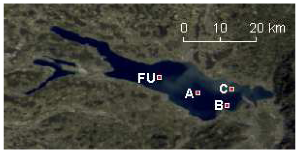
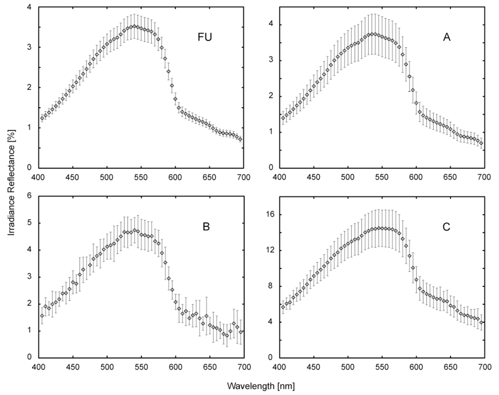
2.2. Field campaign data
2.3. Water quality monitoring data
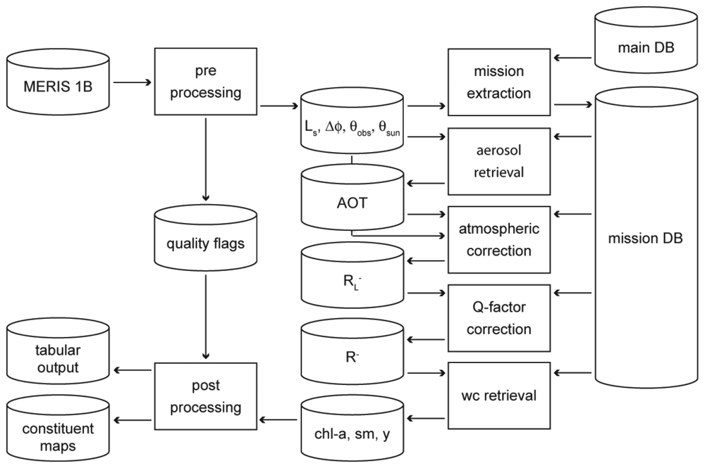
3. Methods
3.1. Algorithm description
3.2. Algorithm parameterization
3.3. Inversion parameterization
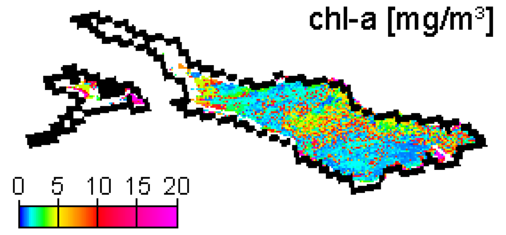
4. Results
4.1. Training of empirical recalibration
4.2. Validation
5. Conclusions and Discussion
Acknowledgments
References and Notes
- Dekker, A.; Malthus, T.J.; Hoogenboom, H.J. The remote sensing of inland water quality. In Advances in Environmental Remote Sensing; Danson, F.M., Plumer, S.E., Eds.; Wiley & Sons: New York, 1995; pp. 123–142. [Google Scholar]
- Doerffer, R.; Schiller, H. The MERIS Case 2 water algorithm. Int. J. Remote Sens. 2007, 28(3), 517–535. [Google Scholar]
- Gege, P.; Plattner, S. MERIS validation activities at Lake Constance in 2003. Proc. of the MERIS User Workshop, Frascati, Italy, 10-13 November 2003; 2004. [Google Scholar]
- Heege, T.; Fischer, J. Mapping of water constituents in Lake Constance using multispectral airborne scanner data and a physically based processing scheme. Can. J. Remote Sensing 2004, 30(1), 77–86. [Google Scholar]
- Heege, T. Flugzeuggestützte Fernerkundung von Wasserinhaltsstoffen am Bodensee; DLR-Forschungsbericht; 2000; Volume 2000, 40, p. 141 pp. (in German) [Google Scholar]
- Liechti, P. Der Zustand der Seen in der Schweiz; BUWAL Schriftenreihe Umwelt; 1994; Volume Nr. 237, p. 159 pp. (in German) [Google Scholar]
- Mürle, U.; Ortlepp, J.; Rey, P. Der Bodensee - Zustand, Fakten, Perspektiven; IGKB, 2004; p. 185 pp. (in German) [Google Scholar]
- Bürgi, H.-R.; Buhmann, D.; Ehmann, H.; Güde, H.; Hetzenauer, H.; Kümmerlin, R.; Kuhn, G.; Obad, R.; Rossknecht, H.; Schröder, H.G.; Stich, H.B.; Wolf, T. Limnologischer Zustand des Bodensees; IGKB Jahresbericht Januar 2005 bis März 2006, 2006; p. 83 pp. (in German) [Google Scholar]
- ESA. MERIS Product Handbook. 2006. http://envisat.esa.int/pub/ESA_DOC/ENVISAT/MERIS/meris.ProductHandbook.2_1.pdf (accessed 20 September 2007).
- Koepke, P. The reflectance factors of a rough ocean with foam. Comment on Remote sensing of the sea state using the 0.8-1.1μm spectral band by Wald, L. and Monget. M. Int. J. Remote Sens. 1985, 6(5), 787–799. [Google Scholar]
- Odermatt, D.; Heege, T.; Nieke, J.; Kneubühler, M.; Itten, K.I. Parameterisation of an automized processing chain for MERIS data of Swiss lakes. Proc. Envisat Symposium, Montreux, Switzerland, 23-27 April 2007; 2007. [Google Scholar]
- TriOS Mess- und Datentechnik GmbH. RAMSES Hyperspectral Radiometer Manual; Rel. 1.0; 2004; p. 27 pp. [Google Scholar]
- Gege, P. Improved method for measuring gelbstoff absorption spectra. Proc.Ocean Optics Conf. XVII, Freemantle, Australia, 25-29 October 2004.
- Stich, H.B.; Brinker, A. Less is better: Uncorrected versus pheopigment-corrected photometric chlorophyll-a estimation. Arch. Hydrobiol. 2005, 162(1), 111–120. [Google Scholar]
- Utermöhl, H. Zur Vervollkommnung der quantitativen Phytoplankton-Methodik. Mitt. Int. Ver. Theor. Angew. Limnol. 1958, 38 pp. (in German). [Google Scholar]
- Tilzer, M.M.; Beese, B. The seasonal productivity cycle of phytoplankton and controlling factors in Lake Constance. Schweiz. Z. Hydrol. 1988, 50(1), 1–39. [Google Scholar]
- Kiselev, V.; Bulgarelli, B. Reflection of light from a rough water surface in numerical methods for solving the radiative transfer equation. J. Quant. Spectrosc. Radiat. Transfer 2004, 85, 419–435. [Google Scholar]
- Gordon, H.R.; Brown, O.B.; Jacobs, M.M. Computed relationships between the inherent and apparent optical properties of a flat homogeneous ocean. Appl. Opt. 1975, 14(2), 417–427. [Google Scholar]
- Kirk, J.T.O. Volume scattering function, average cosines, and the underwater light field. Limnol. Oceanogr. 1991, 36(3), 455–467. [Google Scholar]
- Bannister, T.T. Model of the mean cosine of underwater radiance and estimation of underwater scalar irradiance. Limnol. Oceanogr. 1992, 37(4), 773–780. [Google Scholar]
- Nelder, J.A.; Mead, R. A simplex method for function minimization. Comput. J. 1965, 7, 308–313. [Google Scholar]
- Miksa, S.; Haese, C.; Heege, T. Time series of water constituents and primary production in Lake Constance using satellite data and a physically based modular inversion and processing system. Proc. Ocean Optics Conf. XVIII, Montreal, Canada, 9-13 October 2006.
- Delwart, S. Instrument characterization overview. Presented at NASA/NOAA MERIS US workshop, United States, 14 July 2008.
- Gege, P. Gewässeranalyse mit passiver Fernerkundung: Ein Modell zur Interpretation optischer Spektralmessungen. In DLR-Forschungsbericht; 1994; Volume 1994-15, p. 171 pp. (in German) [Google Scholar]
- Kallio, K.; Pulliainen, J.; Ylöstalo, P. MERIS, MODIS and ETM channel configurations in the estimation of lake water quality from subsurface reflectance with semi-analytical and empirical algorithms. Geophysica 2005, 41, 31–55. [Google Scholar]
- Bricaud, A.; Morel, A.; Prieur, L. Absorption by dissolved organic matter of the sea (yellow substance) in the UV and visible domains. Limnol. Oceanogr. 1981, 26(1), 43–53. [Google Scholar]
- Buiteveld, H.; Hakvoort, J.H.M.; Donze, M. The optical properties of pure water. Proc. Ocean Optics Conf. XII, Bergen, Norway, 13-15 June1994; 2258, pp. 174–183.
- Gege, P. Gaussian model for yellow substance absorption spectra. Proc. Ocean Optics Conf. XV, Monaco, 16-20 October 2000.
- Smith, R.C.; Baker, K. S. Optical properties of the clearest natural waters (200-800 nm). Appl. Opt. 1981, 20(2), 177–184. [Google Scholar]
- Santer, R.; Schmechtig, C. Adjacency Effects on Water Surfaces: Primary Scattering Approximation and Sensitivity Study. Appl. Opt. 2000, 39(3), 361–375. [Google Scholar]
- Candiani, G.; Giardino, C.; Brando, V. Adjacency Effects and bio-optical Model Regionalisation: MERIS Data to assess Lake Water Quality in the Subalpine Region. Proc. Envisat Symposium, Montreux, Switzerland, 23-27 April 2007.


| Band | Wavelength [nm] | Width [nm] | Potential Applications |
|---|---|---|---|
| 1 | 412.5 | 10 | Yellow substance, turbidity |
| 2 | 442.5 | 10 | Chlorophyll absorption maximum |
| 3 | 490 | 10 | Chlorophyll, other pigments |
| 4 | 510 | 10 | Turbidity, suspended sediment, red tides |
| 5 | 560 | 10 | Chlorophyll reference, suspended sediment |
| 6 | 620 | 10 | Suspended sediment |
| 7 | 665 | 10 | Chlorophyll absorption |
| 8 | 681.25 | 7.5 | Chlorophyll fluorescence |
| 9 | 705 | 10 | Atmospheric correction, red edge |
| 10 | 753.75 | 7.5 | Oxygen absorption reference |
| 11 | 760 | 2.5 | Oxygen absorption R-branch |
| 12 | 775 | 15 | Aerosols, vegetation |
| 13 | 865 | 20 | Aerosols corrections over ocean |
| 14 | 890 | 10 | Water vapor absorption reference |
| 15 | 900 | 10 | Water vapor absorption, vegetation |
| Year | Initial set | Sun glint | Cirrus or contrails | MIP error | Working set | Purpose |
|---|---|---|---|---|---|---|
| 2003 | 11 | 1 | 1 | 1 | 8 | Training |
| 2004 | 10 | 2 | 2 | 1 | 5 | Training |
| 2005 | 12 | 3 | 0 | 1 | 8 | Training |
| 2006 | 16 | 2 | 2 | 1 | 11 | IGKB Validation |
| 2007 | 2 | 0 | 1 | 0 | 1 | Field validation |
| Total | 51 | 8 | 6 | 4 | 33 | |
| Process | Parameter | Value |
|---|---|---|
| Atmospheric Correction (LS to RL-) | Aerosol model | Maritime [10] |
| AOT estimation | MERIS channel 14 [10] | |
| sm assumption | 1.5 g/m3 [10] | |
| Water Constituent Retrieval (RL- to chl-a, sm, y) | aw | Buiteveld et al. [27] |
| achl-a | Heege [5]*0.75 | |
| ay | S=0.014 [28] | |
| bw | Smith and Baker [29] | |
| bb, sm | 0.014(λ/400)n n=-0.8(λ/400)1.2 bb/b=0.019 [5] |
| Constituent | Initial value | Min. threshold | Max. threshold |
|---|---|---|---|
| chl-a [mg/m3] | 3 | 0.3 | 20 |
| sm [g/m3] | 1.5 | 0.2 | 10 |
| y [m-1 (440 nm)] | 0.2 | 0.1 | 0.35 |
| Site | UTC | Chl -a [mg/m3] | s m [g/m3] | y [m-1] (400 nm) | |||||
|---|---|---|---|---|---|---|---|---|---|
| UTC ram | situ | ram | mer | situ | ram | mer | ram | mer | |
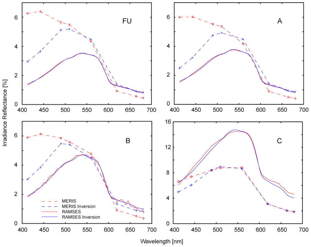
| FU | 8:20 | 0.8 | 1.1 | 1.4 | 0.6 | 0.6 | 0.8 | 0.25 | 0.11 |
| A | 9:25 | 1.1 | 1.9 | 1.1 | 0.8 | 0.7 | 0.7 | 0.21 | 0.10 |
| B | 10:20 | 1.1 | 1.3 | 0.9 | 1.0 | 0.9 | 0.7 | 0.22 | 0.10 |
| C | 11:05 | 3.6 | 4.9 | 3.2 | 2.3 | 3.9 | 1.7 | 0.20 | 0.12 |
| Channel | 1 | 2 | 3 | 4 | 5 | 6 | 7 | 8 | 14 |
|---|---|---|---|---|---|---|---|---|---|
| Recalibration | - | 0.975 | 0.98 | - | - | - | - | - | 0.97 |
| Weighting | - | 0.2 | 0.5 | 1 | 1 | 1 | 1 | 0.8 | 0.97 |
© 2008 by the authors; licensee Molecular Diversity Preservation International, Basel, Switzerland. This article is an open-access article distributed under the terms and conditions of the Creative Commons Attribution license ( http://creativecommons.org/licenses/by/3.0/).
Share and Cite
Odermatt, D.; Heege, T.; Nieke, J.; Kneubühler, M.; Itten, K. Water Quality Monitoring for Lake Constance with a Physically Based Algorithm for MERIS Data. Sensors 2008, 8, 4582-4599. https://doi.org/10.3390/s8084582
Odermatt D, Heege T, Nieke J, Kneubühler M, Itten K. Water Quality Monitoring for Lake Constance with a Physically Based Algorithm for MERIS Data. Sensors. 2008; 8(8):4582-4599. https://doi.org/10.3390/s8084582
Chicago/Turabian StyleOdermatt, Daniel, Thomas Heege, Jens Nieke, Mathias Kneubühler, and Klaus Itten. 2008. "Water Quality Monitoring for Lake Constance with a Physically Based Algorithm for MERIS Data" Sensors 8, no. 8: 4582-4599. https://doi.org/10.3390/s8084582