Connectivity, Coverage and Placement in Wireless Sensor Networks


Abstract
:1. Introduction
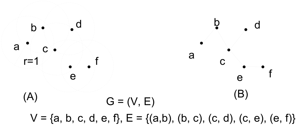
2. Graph Models
3. Connectivity in Wireless Ad Hoc and Sensor Networks
3.1. Percolation in Infinite Graphs
3.2. Connectivity on Finite Graphs
3.3. Techniques to Improve Connectivity
4. Less Regular Connectivity Models
4.1. Non-uniform Disk Radii
4.2. SINR Model
4.3. Shadowing
4.4. Hybrid Models including Wired Infrastructure
5. Relationship between Connectivity and Capacity
5.1. Capacity Constraints imposed by Connectivity
5.2. Improving Capacity by Denser Connectivity
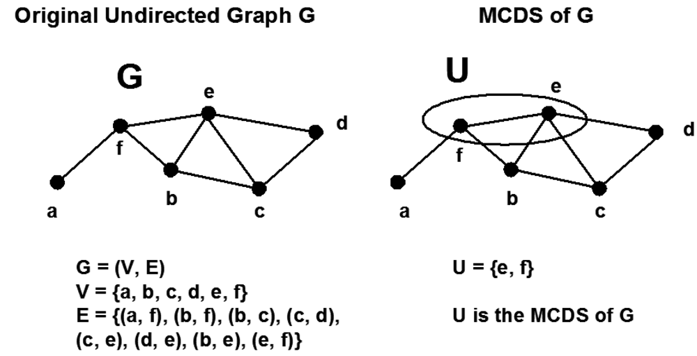
6. Clustering, Virtual Backbone and Minimum Connected Dominating Set
6.1. Cluster Routing Protocols
6.2. Constructive Algorithms
6.3. Pruning-Based Algorithms
6.4. Multipoint Relaying (MPR) in CDS Construction
7. Placement of Nodes
7.1. Placement of Ordinary Nodes
7.2. Placement of Relay Nodes
8. Concluding Remarks
References and Notes
- Whitman, E.C. Sosus: The “Secret Weapon” of Undersea Surveillance. Undersea Warfare. 2005, 7. Available online: http://www.navy.mil/navydata/cno/n87/usw/issue_25/sosus.htm (accessed September 17, 2009).
- Chong, C.Y.; Kumar, S.P. Sensor Networks: Evolution, Opportunities, and Challenges. Proc. IEEE 2003, 91, 1247–1256. [Google Scholar]
- Akyildiz, I.F.; Su, W.; Sankarasubramaniam, Y.; Cayirci, E. Wireless Sensor Networks: A Survey. Comput. Netw. 2002, 38, 393–422. [Google Scholar]
- Sohraby, K.; Minoli, D.; Znati, T. Wireless Sensor Networks: Technology, Protocols and Applications; John Wiley & Sons, Inc.: Hoboken, NJ, USA, 2007. [Google Scholar]
- Ni, S.-Y.; Tseng, Y.-C.; Chen, Y.-S.; Sheu, J.-P. The Broadcast Storm Problem in a Mobile Ad Hoc Network. Proceedings of the 5th Annual ACM/IEEE International Conference on Mobile Computing and Networking, Seattle, Washington, DC, New York, NY, USA; 1999; pp. 151–162. [Google Scholar]
- Raghunathan, V.; Schurgers, C.; Park, S.; Srivastava, M.B. Energy Efficient Design of Wireless Sensor Nodes. In Wireless Sensor Networks; Raghavendra, C.S., Sivalingam, K.M., Znati, T., Eds.; Springer: Berlin / Heidelberg, Germany, 2004; pp. 51–69. [Google Scholar]
- Zhao, Q.; Gurusamy, M. Lifetime Maximization for Connected Target Coverage in Wireless Sensor Networks. IEEE/ACM Trans. Netw. 2008, 16, 1378–1391. [Google Scholar]
- Diestel, R. Graph Theory, electronic edition; Springer-Verlag: Heidelberg, Germany, 2005. [Google Scholar]
- Krohn, A.; Beigl, M.; Decker, C.; Riedel, T.; Zimmer, T.; Varona, D.G. Increasing Connectivity in Wireless Sensor Network using Cooperative Transmission. Proceedings 3rd International Conference on Networked Sensing Systems (INSS), Chicago, IL, USA; 2006. [Google Scholar]
- Bollobás, B. Random Graphs, 2nd ed.; Cambridge University Press: Cambridge, UK, 2001. [Google Scholar]
- Erdős, P.; Rényi, A. On Random Graphs. Publ. Math. 1959, 6, 290–297. [Google Scholar]
- Erdős, P.; Rényi, A. On the Evolution of Random Graphs. Publ. Math. Inst. Hungarian Acad. Sci. 1960, 5, 17–61. [Google Scholar]
- Atay, F.; Stojmenovic, I.; Yanikomeroglu, H. Generating Random Graphs for the Simulation of Wireless Ad Hoc, Actuator, Sensor, and Internet Networks. Proc. 8th IEEE Symposium on a World of Wireless, Mobile and Multimedia Networks WoWMoM, Helsinki, Finland, June 2007.
- Dowell, L.J.; Bruno, M.L. Connectivity of Random Graphs and Mobile Networks: Validation of Monte Carlo Simulation Results. Proc. the 2001 ACM symposium on Applied computing (SAC '01), ACM, New York, NY, USA, March 2001.
- Gkantsidis, C.; Mihail, M.; Zegura, E. The Markov Chain Simulation Method for Generating Connected Power Law Random Graphs. Proc. 5th SIAM Workshop on Algorithm Engineering and Experiments (ALENEX), Baltimore, MA, USA, January 2003.
- Ioannides, Y.M. Random Graphs and Social Networks: An Economics Perspective. Available online: http://ase.tufts.edu/econ/papers/200518.pdf (accessed on April 1, 2008).
- Newman, M.E.J.; Watts, D.J.; Strogatz, S.H. Random Graph Models of Social Networks. Proc Nat Acad Sci, USA 2002, 99 Suppl. 1, 2566–2572. [Google Scholar]
- Saul, Z.M.; Filkov, V. Exploring Biological Network Structure Using Exponential Random Graph Models. Bioinformatics 2007, 23, 2604–2611. [Google Scholar]
- Gilbert, E.N. Random Graphs. Ann. Math. Statist. 1959, 30, 1141–1144. [Google Scholar]
- Austin, T.L.; Fagen, R.E.; Penney, W.F.; Riordan, J. The Number of Components in Random Linear Graphs. Ann. Math. Statist. 1959, 30, 747–754. [Google Scholar]
- Ford, G.W.; Uhlenbeck, G.E. Combinatorial Problems in the Theory of Graphs. Proc. Nat. Acad. Sci. USA 1957, 43, 163–167. [Google Scholar]
- Chlamtac, I.; Faragó, A. A New Approach to the Design and Analysis of Peer-to-Peer Mobile Networks. ACM Wirel. Netw. 1999, 5, 149–156. [Google Scholar]
- Penrose, M.D. Random Geometric Graphs; Oxford University Press: Oxford, UK, 2003. [Google Scholar]
- Gilbert, E.N. Random Plane Networks. SIAM J. 1961, 9, 533–543. [Google Scholar]
- Gupta, P.; Kumar, P.R. Critical Power for Asymptotic Connectivity in Wireless Networks. In Stochastic Analysis, Control, Optimization and Applications: A Volume in Honor of W.H. Fleming; McEneaney, W.M., Yin, G.G., Zhang, Q., Eds.; Birkhauser Boston: Cambridge, MA, USA, 1998; pp. 1106–1110. [Google Scholar]
- Gupta, P.; Kumar, P.R. The Capacity of Wireless Networks. IEEE Trans. Inform. Theory 2000, 46, 388–404. [Google Scholar]
- Ozgur, A.; Leveque, O.; Tse, D. Hierarchical Cooperation Achieves Linear Capacity Scaling in Ad Hoc Networks. Proc. 26th IEEE International Conference on Computer Communications (INFOCOM'07, Anchorage, Alaska, USA, May 2007; pp. 382–390.
- Hall, P. On Continuum Percolation. Ann. Probab. 1985, 13, 1250–1266. [Google Scholar]
- Menshikov, M.V. Coincidence of Critical Points in Percolation Problems. Soviet Math. Dokl. 1986, 24, 856–859. [Google Scholar]
- Broadbent, S.R. Discussion on Symposium on Monte Carlo Methods. J. Roy. Statist. Soc., Ser. B 1954, 16, 61–75. [Google Scholar]
- Broadbent, S.R.; Hammersley, J.M. Percolation Processes, I. Crystals and Mazes. Proceedings of The Cambridge Philosophical Society, Cambridge, UK; 1957; 53, pp. 629–641. [Google Scholar]
- Hammersley, J.M. Percolation Processes, II. The Connective Constant. Proceedings Of The Cambridge Philosophical Society, Cambridge, UK; 1957; 53, pp. 642–645. [Google Scholar]
- Philips, T.K.; Panwar, S.S.; Tantawi, A.N. Connectivity Properties of a Packet Radio Network Model. IEEE Trans. Inform. Theory 1989, 35, 1044–1047. [Google Scholar]
- Quintanilla, S.; Torquato, S.; Ziff, R.M. Efficient Measurement of the Percolation Threshold for Fully Penetrable Discs. J. Phys. A: Math. Gen. 2000, 33, L399–L407. [Google Scholar]
- Santi, P.; Blough, D.M. The Critical Transmitting Range for Connectivity in Sparse Wireless Ad Hoc Networks. IEEE Trans. Mobile Comput. 2003, 2, 1–15. [Google Scholar]
- Hekmat, R.; Mieghem, P.V. Connectivity in Wireless Ad-Hoc Networks with A Log-normal Radio Model. Mobile Netw. Appl. 2006, 11, 351–360. [Google Scholar]
- Ta, X.; Mao, G.; Anderson, B.D.O. On the Properties of Giant Component in Wireless Multi-hop Networks. Proceedings 28th IEEE Infocom'09 mini-conference, Rio de Janeiro, Brazil, April 2009.
- Han, G.; Makowski, A.M. One-dimensional Geometric Random Graphs with Non-vanishing Densities I: A Strong Zero-one Law for Connectivity. IEEE Trans. Inform. Theory 2009, in press. [Google Scholar]
- Han, G.; Makowski, A.M. Sensitivity of Critical Transmission Ranges to Node Placement Distributions. IEEE J. Sel. Area. Comm. 2009, in press. [Google Scholar]
- Piret, P. On the Connectivity of Radio Networks. IEEE Trans. Inform. Theory 1991, 37, 1490–1492. [Google Scholar]
- Penrose, M.D. On k-Connectivity for a Geometric Random Graph. Random Struct. Algor. 1999, 15, 145–164. [Google Scholar]
- Bettstetter, C. On the Minimum Node Degree and Connectivity of a Wireless Multihop Network. Proc. 3rd ACM International Symposium on Mobile Ad Hoc Networking and Computing (MobiHoc 02), ACM, New York, NY, USA; 2002; pp. 80–91. [Google Scholar]
- Desai, M.; Manjunath, D. On the Connectivity in Finite Ad Hoc Networks. IEEE Comm. Lett. 2002, 6, 437–439. [Google Scholar]
- Gore, A.D. Comments on “On the Connectivity in Finite Ad Hoc Networks”. IEEE Comm. Lett. 2006, 10, 88–90. [Google Scholar]
- Gore, A.D. Correction to “Comments on 'On the Connectivity in Finite Ad Hoc Networks’”. IEEE Comm. Lett. 2006, 10, 359. [Google Scholar]
- Foh, C.H.; Lee, B.S. A Closed Form Network Connectivity Formula for One-Dimensional MANETs. Proc. IEEE Int. Conf. Comm. (ICC) 2004, 6, 3739–3742. [Google Scholar]
- Li, J.; Andrew, L.H.L.; Foh, C.H.; Zukerman, M.; Neuts, M.F. Meeting Connectivity Requirements in a Wireless Multihop Network. IEEE Comm. Lett. 2006, 10, 19–21. [Google Scholar]
- Scaglione, A.; Hong, Y.-W. Opportunistic Large Arrays: Cooperative Transmission in Wireless Multihop Ad Hoc Networks to Reach Far Distances. IEEE Trans. Signal Process. 2003, 51, 2082–2092. [Google Scholar]
- Kranakis, E.; Krizanc, D.; Williams, E. Directional Versus Omnidirectional Antennas for Energy Consumption and k-Connectivity of Networks of Sensors. Lect. Note. Comput. Sci. 2005, 3544, 357–368. [Google Scholar]
- Bhattacharya, B.; Hu, Y.; Shi, Q.; Kranakis, E.; Krizanc, D. Sensor Network Connectivity with Multiple Directional Antennae of a Given Angular Sum. Proceedings 23rd IEEE International Parallel and Distributed Processing Symposium (IPDPS 2009), Rome, Italy, May 2009.
- Xue, F.; Kumar, P.R. The Number of Neighbors Needed for Connectivity of Wireless Networks. Wirel. Netw. 2004, 10, 169–181. [Google Scholar]
- Ganesh, A.; Xue, F. On the Connectivity and Diameter of Small-World Networks. Adv. Appl. Probab. 2007, 39, 853–863. [Google Scholar]
- Blough, D.M.; Leoncini, M.; Resta, G.; Santi, P. The K-Neigh Protocol for Symmetric Topology Control in Ad Hoc Networks. Proceedings of the 4th ACM international symposium on Mobile ad hoc networking and computing, Annapolis, Maryland, USA; 2003; pp. 141–452. [Google Scholar]
- Bettstetter, C. On the Connectivity of Wireless Multihop Networks with Homogeneous and Inho-mogeneous Range Assignment. Proceedings of IEEE 56th Vehicular Technology Conference (VTC-2002, Fall), Vancouver, British Columbia, Canada; 2002; 3, pp. 1706–1710. [Google Scholar]
- Sanchez, M.; Manzoni, P.; Haas, Z.J. Determination of Critical Transmitting Ranges in Ad Hoc Networks. Proc. Multiaccess, Mobility and Teletraffic for Wireless Communications Conference, New Orleans, LA, USA; 1999. [Google Scholar]
- Santi, P. The Critical Transmitting Range for Connectivity in Mobile Ad Hoc Networks. IEEE Trans. Mobile Comput. 2005, 4, 310–317. [Google Scholar]
- Wan, P.J.; Yi, C.W. Asymptotic Critical Transmission Radius and Critical Neighbor Number for k-Connectivity in Wireless Ad Hoc Networks. Proceedings of the 5th ACM international symposium on Mobile ad hoc networking and computing, Roppongi Hills, Tokyo, Japan; 2004; pp. 1–8. [Google Scholar]
- Dousse, O.; Baccelli, F.; Thiran, P. Impact of Interferences on Connectivity in Ad Hoc Networks. IEEE/ACM Trans. Netw. (TON) 2005, 13, 425–436. [Google Scholar]
- Rappaport, T.S. Wireless Communications Principles and Practice, 2nd ed.; Pearson Education: Upper Saddle River, NJ, USA, 2004. [Google Scholar]
- Zorzi, M.; Pupolin, S. Optimum Transmission Ranges in Multihop Packet Radio Networks in the presence of Fading. IEEE Trans. Comm. 1995, 43, 2201–2205. [Google Scholar]
- Bettstetter, C.; Hartmann, C. Connectivity of Wireless Multihop Networks in a Shadow Fading Environment. Proc. 6th ACM International Workshop on Modeling, Analysis and Simulation of Wireless and Mobile Systems, San Diego, CA, USA, September 19, 2003; pp. 28–32.
- Booth, L.; Bruck, J.; Cook, M.; Franceschetti, M. Ad Hoc Wireless Networks with Noisy Links. Proc. IEEE International Symposium on information Theory, 2003, Yokohama, Japan, June 29–July 4, 2003.
- Booth, L.; Bruck, J.; Cook, M.; Franceschetti, M. Covering Algorithms, Continuum Percolation and the Geometry of Wireless Networks. Ann. Appl. Probab. 2003, 13, 722–731. [Google Scholar]
- Dousse, O.; Thiran, P.; Hasler, M. Connectivity in Ad-Hoc and Hybrid Networks. Proc. IEEE INFOCOM 2002, New York, NY, USA, June 23–27, 2002; 2, pp. 1079–1088.
- Franceschetti, M.; Dousse, O.; Tse, D.; Thiran, P. Closing the Gap in the Capacity of Wireless Networks via Percolation Theory. IEEE Trans. Inf. Theory 2007, 53, 1009–1018. [Google Scholar]
- Dousse, O.; Franceschetti, M.; Thiran, P. Information Theoretic Bounds on the Throughput Scaling of Wireless Relay Networks. Proc. IEEE INFOCOM 2005. 24th Annual Joint Conference of the IEEE Computer and Communications Societies, Miami, FL, USA; 2005; 4, pp. 2670–2678. [Google Scholar]
- Dousse, O.; Thiran, P. Connectivity vs Capacity in Dense Ad Hoc Networks. Proc. INFOCOM 2004. 23rd Annual Joint Conference of the IEEE Computer and Communications Societies, Hong Kong, China, March 2004.
- Kleinrock, L.; Silvester, J. Optimum Transmission Radii for Packet Radio Networks or Why Six is a Magic Number. Proc. National Telecommunications Conference, Birmingham, Al, USA, December 1978.
- Takagi, H.; Kleinrock, L. Optimal Transmission Ranges for Randomly Distributed Packet Radio Terminals. IEEE Trans. Comm. 1984, 32, 246–257. [Google Scholar]
- Hajek, B. Adaptive Transmission Strategies and Routing in Mobile Radio Networks. Proc. Conference on Information Sciences and Systems, Princeton, NJ, USA, March 1983; pp. 372–378.
- Hou, T.; Li, V. Transmission Range Control in Multihop Packet Radio Networks. IEEE Trans. Comm. 1986, 34, 38–44. [Google Scholar]
- Hedrick, C. RFC1058 - Routing Information Protocol. Internet Request for Comments: 1058. June 1998. Available online: http://www.faqs.org/rfcs/rfc1058.html (accessed September 18, 2009).
- Moy, J. OSPF Version 2; Internet Request For Comments: RFC 1247. July 1991. Available online: http://www.ietf.org/rfc/rfc1247.txt (accessed September 18, 2009).
- Biswas, S.; Morris, R. Exor: Opportunistic Routing in Multihop Wireless Networks. Proc. of ACM SIGCOMM, Philadelphia, PA, USA, August 2005; pp. 133–144.
- Cui, T.; Chen, L.; Ho, T.; Low, S.H.; Andrew, L.L.H. Opportunistic Source Coding for Data Gathering in Wireless Sensor Networks. Proc. IEEE Mobile Ad-hoc and Sensor Systems (MASS), Pisa, Italy, October 8–11, 2007; pp. 1–11.
- Tubaishat, M.; Madria, S. Sensor Networks: an Overview. IEEE Potent. 2003, 22, 20–23. [Google Scholar]
- Heinzelman, W.; Chandrakasan, A.; Balakrishnan, H. Energy-efficient Communication Protocol for Wireless Microsensor Networks. Proc. Hawaii International Conf. on Systems Science, Maui, Hawaii, USA, January 2000.
- Hussain, S.; Matin, A.W. Hierarchical Cluster-based Routing in Wireless Sensor Networks. Proc. International Conference on Information Processing in Sensor Networks (IPSN 2006), Nashville, TN, USA; 2006. [Google Scholar]
- Jiang, M.; Li, J.; Tay, Y. Cluster Based Routing Protocol (CBRP) Functional Specification. In IETF Internet Draft; MANET working group, August 1999. [Google Scholar]
- Sivakumar, R.; Sinha, P.; Bharghavan, V. CEDAR: A Core-Extraction Distributed Ad Hoc Routing Protocol. IEEE J. Sele. Area. Comm. 1999, 17, 1454–1465. [Google Scholar]
- Manjeshwar, A.; Agrawal, D. TEEN: A Protocol for Enhanced Efficiency in WSNs. Proc. the First International Workshop on Parallel and Distributed Computing Issues in Wireless Networks and Mobile Computing, San Francisco, CA, USA, April 2001.
- Manjeshwar, A.; Agrawal, D. APTEEN: A Hybrid Protocol for Efficient Routing and Comprehensive Information Retrieval in WSNs. Proc. 2nd International Parallel and Distributed Computing Issues in Wireless Networks and Mobile Computing, Ft. Lauderdale, FL, USA, April 2002; pp. 195–202.
- Johnson, D. B.; Maltz, D.A. Dynamic Source Routing in Ad Hoc Wireless Networks. Mobile Comput. 1996, 353, 153–181. [Google Scholar]
- Perkins, C. E.; Royer, E. M. Ad Hoc On-Demand Distance Vector Routing. Proceedings of IEEE Workshop on Mobile Computing Systems and Applications, New Orleans, LA, USA, February 1999; pp. 90–100.
- Das, B.; Sivakumar, E.; Bhargavan, V. Routing in Ad Hoc Networks Using a Virtual Backbone. Proceedings fo the 6th International Conference on Computer Communications and Networks (IC3N'97), Las Vegas, NV, USA, September 22–25, 1997.
- Wang, Y.; Wang, W.; Li, X.Y. Distributed Low-cost Backbone Formation for Wireless Ad Hoc Networks. Proc. 6th ACM International Symposium on Mobile Ad Hoc Networking and Computing (MobiHoc05), Urbana-Champaign, IL, USA; 2005; pp. 2–13. [Google Scholar]
- Garey, M.R.; Johnson, D.S. Computers and Intractability: A Guide to the Theory of NP-Completeness; Freeman, W.H., Ed.; San Francisco, CA, USA, 1979. [Google Scholar]
- Li, J.; Andrew, L.H.L.; Foh, C.H.; Zukerman, M. Sizes of Minimum Connected Dominating Sets of a Class of Wireless Sensor Networks. Proceedings of IEEE International Conference on Communications, Beijing, China, May 2008.
- Guha, S.; Khuller, S. Approximation Algorithms for Connected Dominating Sets. Algorithmica 1998, 20, 374–387. [Google Scholar]
- Graham, R.L.; Knuth, D.E.; Patashnik, O. Concrete Mathematics: A Foundation for Computer Science, 2nd ed.; Pearson Education: Upper Saddle River, NJ, USA, 2002. [Google Scholar]
- Dijkstra, E. A note on Two Problems in Connection with Graphs. Numb. Math. 1959, 1, 269–271. [Google Scholar]
- Cartigny, J.; Simplot, D.; Stojmenovic, I. Localized Minimum-Energy Broadcasting in Ad-Hoc Networks. Proc. Twenty-Second Annual Joint Conference of the IEEE Computer and Communications Societies, IEEE INFOCOM 2003, San Francisco, CA, USA; 2003; 3, pp. 2210–2217. [Google Scholar]
- Das, B.; Bharghavan, V. Routing in Ad-Hoc Networks Using Minimum Connected Dominating Sets. Proc. IEEE Int. Conf. Comm. (ICC) 1997, 376–380. [Google Scholar]
- Alzoubi, K.M.; Wan, P.J.; Frieder, O. Distributed Heuristics for Connected Dominating Sets in Wireless Ad Hoc Networks. J. Comm. Netw. 2002, 4, 15–19. [Google Scholar]
- Marathe, M.V.; Breu, H.; Hunt, H.B., III; Ravi, S.S.; Rosenkrantz, D.J. Simple Heuristics for Unit Disk Graphs. Networks 1995, 25, 59–68. [Google Scholar]
- Alzoubi, K.M.; Wan, P.J.; Frieder, O. Message Optimal Connected Dominating Sets in Mobile Ad Hoc Networks. Proc. 3rd ACM International Symposium of Mobile Ad Hoc Networks and Computing (MobiHoc 02), Lausanne, Switzerland, June 2002; pp. 157–164.
- Butenko, S.; Cheng, X.; Du, D.Z.; Pardalos, P.M. On the Construction of Virtual Backbone for Ad Hoc Wireless Networks. In Cooperative Control: Models, Applications and Algorithms; Butenko, S., Murphey, R., Pardalos, P.M., Eds.; Kluwer Academic Publishers: Norwell, MA, USA, 2003; pp. 43–54. [Google Scholar]
- Cadei, M.; Cheng, X.; Du, D.Z. Connected Domination in Ad Hoc Wireless Networks. Proc. 6th International Conference on Computer Science and Informatics, Durham, NC, USA; 2002. [Google Scholar]
- Ou, L.; Sekercioglu, Y.A.; Mani, N. A Low-cost Flooding Algorithm for Wireless Sensor Networks. Proc. Wireless communications and Networking Conference, 2007 (WCNC 2007), Hong Kong, China, March 2007.
- Wu, J.; Li, H. On Calculating Connected Dominating set for Efficient Routing in Ad Hoc Wireless Networks. Proc. 3rd International Workshop on Discrete Algorithms and Methods for Mible Computing and Communications, New York, NY, USA, August 1999; pp. 7–14.
- Wu, J.; Gao, M.; Stojmenovic, I. On Calculating Power-Aware Connected Dominating Sets for Efficient Routing in Ad Hoc Wireless Networks. Proc. 2001 International Conference of Parallel Processing, Las Vegas, NV, USA; 2001; pp. 346–356. [Google Scholar]
- Butenko, S.; Cheng, X.; Oliveira, C.; Pardalos, P.M. A New Heuristic for the Minimum Connected Dominating Set Problem on Ad Hoc Wireless Networks. In Recent Developments in Cooperative Contral and Optimization; Butenko, S., Murphey, R., Pardalos, P., Eds.; Kluwer Academic Publishers: Norwell, MA, USA, 2004; Chapter 4; pp. 61–73. [Google Scholar]
- Sanchis, L.A. Experimental Analysis of Heuristic Algorithms for the Dominating Set Problem. Algorithmica 2002, 33, 3–18. [Google Scholar]
- Qayyum, A.; Viennot, L.; Laouiti, A. Multipoint Relaying for Flooding Broadcast Messages in Mobile Wireless Networks. Proc. 35th Hawaii International Conference on System Sciences, Hawaii, NJ, USA, January 2002; pp. 3866–3875.
- Adjih, C.; Jacquet, P.; Viennot, L. Computing Connected Dominated Sets with Multipoint Relays. Ad Hoc Sensor Netw. 2005, 1, 27–39. [Google Scholar]
- Wu, J. An Enhanced Approach to determine a small Forward Node Set Based on Multipoint Relays. Proc. 2003 IEEE 58th Vehicular Technology Conference, VTC 2003-Fall, Orlando, Florida, USA, October 2003; 4, pp. 2774–2777.
- Chen, X.; Shen, J. Reducing Connected Dominating Set Size with Multipoint Relays in Ad Hoc Wireless Networks. Proc. 7th International Symposium on Parallel Architectures, Algorithms and Networks (ISPAN'04), Hong Kong, China, May 2004; pp. 539–543.
- Wu, J. Extended Dominating-Set-Based Routing in Ad Hoc Wireless Networks with unidirectional Links. IEEE T. Parall. Distr. 2002, 9, 866–881. [Google Scholar]
- Wu, J.; Lou, W.; Dai, F. Extended Multipoint Relays to Determine Connected Dominating Sets in MANETs. IEEE Trans. Comput. 2006, 55, 334–347. [Google Scholar]
- Ou, L.; Şekercioğlu, Y.A.; Mani, N. A Survey of Multipoint Relay Based Broadcast Schemes in Wireless Ad Hoc Networks. IEEE Communications Surveys and Tutorials 2006, 8, 30–46. [Google Scholar]
- Dhillon, S.S.; Chakrabarty, K. Sensor Placement for Effective Coverage and Surveillance in Distributed Sensor Networks. Proc. IEEEWireless Communications and Networking, 2003 (WCNC 2003), New Orleans, LA, USA, March 2003; 3, pp. 1609–1614.
- O'Rourke, J. Art Gallery Theorems and Algorithms; Oxford University Press, Inc.: New York, NY, USA, 1987. [Google Scholar]
- Gonzólez-Banos, H. Randomized Art-Gallery Algorithm for Sensor Placement. Proceedings of the 7th Annual Symposium on Computational Geometry, Medford, Massachusetts, USA; 2001; pp. 232–240. [Google Scholar]
- Zhang, H.; Hou, J.C. Maintaining Sensing Coverage and Connectivity in Large Sensor Networks. Ad Hoc Sensor Wirel. Netw. 2005, 1, 89–124. [Google Scholar]
- Kershner, R. The Number of Circles Covering a Set. Am. J. Math. 1939, 61, 665–671. [Google Scholar]
- Chen, J.; Li, S.; Sun, Y. Novel Deployment Schemes for Mobile Sensor Networks. Sensors 2007, 7, 2907–2919. [Google Scholar]
- Coskun, V. Relocating Sensor Nodes to Maximize Cumulative Connected Coverage in Wireless Sensor Networks. Sensors 2008, 8, 2792–2817. [Google Scholar]
- Aitsaadi, N.; Achir, N.; Boussetta, K.; Pujolle, G. A Tabu Search WSN Deployment Method for Monitoring Geographically Irregular Distributed Events. Sensors 2009, 9, 1625–1643. [Google Scholar]
- Biagioni, E.S.; Sasaki, G. Wireless Sensor Placement for Reliable and Efficient Data Collection. Proc. 36th Annual Hawaii International Conference on System Sciences, Big Island, HI, USA, January 2003.
- Iyengar, R.; Kar, K.; Banerjee, S. Low-coordination Topologies for Redundancy in Sensor Networks. Proc. MobiHoc'05, Urbana-Champaign, IL, USA, May 2005.
- Bai, X.; Santosh, K.; Dong, X.; Yun, Z.; Ten, H.L. Deploying Wireless Sensors to Achieve Both Coverage and Connectivity. Proc. of the 7th ACM International Symposium on Mobile ad hoc networking and computing MobiHoc'06, Florence, Italy, May, May 22–25, 2006.
- Bai, X.; Xuan, D.; Yun, Z.; Lai, T.H.; Jia, W. Complete Optimal Deployment Patterns for Full-Coverage and k-Connectivity (k ≤ 6) Wireless Sensor Networks. Proceedings of the 9th ACM international symposium on Mobile ad hoc networking and computing, Hong Kong, China, May 2008; pp. 401–410.
- Wang, Y.C.; Hu, C.C.; Tseng, Y.C. Efficient Deployment Algorithms for Ensuring Coverage and Connectivity of Wireless Sensor Networks. Proc. First International Conference on Wireless Internet, Visegrad-Budapest, Hungary, July 2005; pp. 114–121.
- Khan, S.U. Approximate Optimal Sensor Placements in Grid Sensor Fields. Proc. IEEE 65th Vehicular Technology Conference, 2007. VTC2007-Springer, Dublin, Ireland, April 2007; pp. 248–251.
- Chakrabarty, K.; Iyengar, S.S.; Qi, H.; Cho, E. Grid Coverage for Surveillance and Target Location in Distributed Sensor Networks. IEEE Trans. Comp. 2002, 51, 1448–1453. [Google Scholar]
- Lin, F.Y.S.; Chiu, P.L. A Near-Optimal Sensor Placement Algorithm to Achieve Complete Coverage/Discrimination in Sensor Networks. IEEE Comm. Lett. 2005, 9, 43–45. [Google Scholar]
- Ishizuka, M.; Aida, M. Performance Study of Node Placement in Sensor Networks. Proceedings. 24th International Conference on Distributed Computing Systems Workshops, 2004, Hachioji, Tokyo, Japan, March 2004; pp. 598–603.
- Miller, L.E. Distribution of Link Distances in a Wireless Network. J. Res. Natl. Instit. Stan. 2001, 106, 401–412. [Google Scholar]
- Blough, D.M.; Resta, G.; Santi, P. A Statistical Analysis of the Long-run Node Spatial Distribution in Mobile Ad Hoc Networks. Wirel. Netw. 2004, 10, 543–554. [Google Scholar]
- Cheng, X.; Du, D.Z.; Wang, L.; Xu, B. Relay Sensor Placement in Wireless Sensor Networks. Wirel. Netw. 2008, 14, 347–355. [Google Scholar]
- Hao, B.; Tang, J.; Xue, G. Fault-Tolerant Relay Node Placement in Wireless Sensor Networks: Formulation and Approximation. Proc. IEEE Workshop High performance switching and routing (HPSR'04; 2004; pp. 246–250. [Google Scholar]
- Pan, J.; Hou, Y.T.; Cai, L.; Shi, Y.; Shen, S.X. Topology control for Wireless Sensor Networks. Proc. ACM Mobicom'03, San Diego, CA, USA; 2003; pp. 286–299. [Google Scholar]
- Tang, J.; Hao, B.; Sen, A. Relay Node Placement in Large Scale Wireless Sensor Networks. Comput. Comm.s 2006, 29, 490–501. [Google Scholar]
- Zhang, W.; Xue, G.; Misra, S. Fault-Tolerant Relay Node Placement in Wireless Sensor Networks: Problems and Algorithms. Proc. 26th IEEE International Conference on Computer Communications (INFOCOM 2007), Anchorage, AK, USA, May 2007; pp. 1649–1657.
- Lin, G.; Xue, G. Steiner Tree Problem with Minimum Number of Steiner Points and Bounded Edge-Length. Inf. Proc. Lett. 1999, 69, 53–57. [Google Scholar]
- Chen, D.; Du, D.Z.; Hu, X.D.; Lin, G.; Wang, L.; Xue, G. Approximations for Steiner Trees with Minimum Number of Steiner Points. J. Glob. Opt. 2000, 18, 17–33. [Google Scholar]
- Kashyap, A.; Khuller, S.; Shayman, M. Relay Placement for Higher Order Connectivity in Wireless Sensor Networks. Proceedings 25th IEEE International Conference on Computer Communications (INFOCOM2006), Barcelona, Spain; 2006; pp. 1–12. [Google Scholar]
- Lloyd, E.L.; Xue, G. Relay Node Placement in Wireless Sensor Networks. IEEE Trans. Comoput. 2007, 56, 134–138. [Google Scholar]
- Misra, S.; Hong, S.D.; Xue, G.; Tang, J. Constrained Relay Node Placement in Wireless Sensor Networks to Meet Connectivity and Survivability Requirements. Proc. IEEE 27th Conference on Computer Communications (INFOCOM 2008), Phoenix, AZ, USA, April 2008; pp. 281–285.
- Srinivas, A.; Modiano, E. Joint Node Placement and Assignment for Throughput Optimization in Mobile Backbone Networks. Proc. IEEE 27th Conference on Computer Communications (INFOCOM 2008), Phoenix, AZ, USA, April 2008; pp. 1130–1138.


© 2009 by the authors; licensee Molecular Diversity Preservation International, Basel, Switzerland. This article is an open access article distributed under the terms and conditions of the Creative Commons Attribution license (http://creativecommons.org/licenses/by/3.0/).
Share and Cite
Li, J.; Andrew, L.L.H.; Foh, C.H.; Zukerman, M.; Chen, H.-H. Connectivity, Coverage and Placement in Wireless Sensor Networks. Sensors 2009, 9, 7664-7693. https://doi.org/10.3390/s91007664
Li J, Andrew LLH, Foh CH, Zukerman M, Chen H-H. Connectivity, Coverage and Placement in Wireless Sensor Networks. Sensors. 2009; 9(10):7664-7693. https://doi.org/10.3390/s91007664
Chicago/Turabian StyleLi, Ji, Lachlan L.H. Andrew, Chuan Heng Foh, Moshe Zukerman, and Hsiao-Hwa Chen. 2009. "Connectivity, Coverage and Placement in Wireless Sensor Networks" Sensors 9, no. 10: 7664-7693. https://doi.org/10.3390/s91007664