1. Introduction
With the advancements of Micro-Electro-Mechanical System (MEMS), digital electronics, as well as wireless communication technology, a kind of small-size, low-cost, and low-power device with sensing, processing and wireless transmission capabilities, called
sensor, is widely developed and deployed in a variety of applications. A wireless sensor network (WSN) is an auto-configured network consisted of many sensors deployed in a sensing field in an ad hoc or prearranged fashion. The purposes of WSNs include sensing, monitoring, or tracking environmental events. WSNs have been widely used in battlefield surveillance, environmental monitoring, biological detection, home automation, industrial diagnostics, etc. [
1].
A wireless heterogeneous sensor network (WHSN) is a sub-class of wireless sensor networks in which each sensor may have different capabilities, such as various transmission capabilities, different number of sensing units, etc. [
2,
3]. In the paper, a WHSN with multiple sensing units is considered, which means each sensor in the WHSN may be equipped with more than one sensing unit, and the
attribute that each sensing unit can sense may also be different. In fact, sensors equipped with multiple sensing units are very common in many commercial products. For example, each MICA2 mote [
4] is equipped with several sensing units for temperature, humidity, light, sound, vibration, etc. A WHSN with multiple sensing units is inherently formed in nature because some sensing units in a sensor may be malfunctioned after running for a long time. The remaining sensing units on each sensor may be different. As a result, how to utilize the sensors with the remaining sensing units efficiently to continue the original sensing task is a very important concern.
Furthermore, using a WHSN with multiple sensing units is also cost-effective and power-efficient if multiple attributes are required to be sensed in the sensing field. On one hand, in addition to the sensing unit, a sensor, in general, consists of a control unit, a power unit, a radio unit, etc. If a sensor is equipped with only one sensing unit, it will increase the cost substantially to deploy all kinds of sensors to sense all required attributes. On the other hand, if too many sensing units are equipped in a sensor, the sensor will quickly run out of energy. Therefore, a WHSN with multiple sensing units is a promising deployment if multiple attributes are required to be sensed in the sensing field [
2,
3]. Moreover, it is very likely that several different kinds of sensors have been deployed in the sensing field for different purposes. These sensors can collaborate for additional sensing purposes to increase the sensor utilization.
Coverage and
connectivity are two key factors to a successful WSN. In general, coverage problems either deploy sensors to cover the sensing field completely [
5,
6], or make sure that all the sensing field is covered by a certain amount of sensors, such as 1-coverage or
k-coverage [
7,
8], or select active sensors in a densely deployed sensor networks to cover all the sensing field [
9–
12]. On the other hand, the connectivity issue emphasizes how well sensors connect to the sink and if the sensed data can be properly delivered to the sink. The connected target coverage (CTC) problem is one of the target coverage (TC) problems, but also takes the connectivity issue into consideration simultaneously. In this paper, CTC problem in a WHSN with multiple sensing units is termed MU-CTC problem (where MU means multiple sensing units) and is defined as below.
Definition 1 (MU-CTC Problem) Given a set of targets (or points) of interest and a number of sensors with multiple sensing units randomly deployed in the sensing field, MU-CTC problem is to schedule the on/off of the sensing units as well as the communication unit on each sensor such that (1) the attributes required to be sensed at each target can be sensed at all time, (2) the sensed data can be delivered to the sink, and (3) the network lifetime is maximized.
The network lifetime is defined as the time interval from the beginning to the time that either the condition (1) or (2) above is not satisfied.
MU-CTC problem can be represented by a bipartite graph and be reduced to a connected set cover problem, named MU-CSC (
Multiple sensing
Units for
Connected
Set
Cover) problem. The MU-CSC problem can be formulated as an integer linear programming (ILP) problem and solved by an ILP solver. However, solving the ILP problem is NP-complete [
13]. Therefore, two distributed schemes, named REFS (remaining energy first scheme) and EEFS (energy efficiency first scheme), are proposed to deal with the MU-CTC problem. In REFS, a sensor enables its sensing and communication units based on its remaining energy and its neighbors’ decisions. The advantages of REFS are its simplicity and reduced communication overhead. However, redundant sensing is the most significant weakness of REFS.
Generally in the CTC problem, a sensor not only undertakes the sensing task, but also needs to relay the sensed data for others. Therefore, to make the best use of a sensor’s energy, target coverage and sensed data relay should be considered simultaneously. Consequently, EEFS is proposed, where a sensor enables its sensing and communication units by considering not only its target coverage but also its relay role. As a result, the network lifetime of EEFS can be prolonged accordingly. Simulation results also verify that EEFS outperforms REFS in network lifetime. In addition, to our best knowledge, this is the first paper to discuss such a problem in the literature.
The rest of the paper is organized as follows. Section 2 describes the related work that treated the CTC problem with different network models and assumptions. Section 3 formulates MU-CTC problem as an ILP problem. Section 4, two distributed schemes, REFS and EEFS, are proposed to deal with the MU-CTC problem. Simulation results are presented in Section 5. Section 6 concludes the paper.
2. Related Work
Coverage problem is of critical importance for wireless sensor networks. As described above, the coverage problem either deploys sensors to cover the sensing field, or selects active sensors and schedule them to cover all the sensing field, or analyzes how well the sensing field is covered. Recently, the target coverage problem has received extensive attention [
13–
20]. Nevertheless, none of them considered sensors equipped with multiple sensing units. Moreover, some of them do not take the connectivity issue into account. These researches are summarized as follows.
In [
13], the authors transformed the TC problem into a
Maximal Set Cover (MSC) problem, where sensors are organized into set covers. To maximize the number of set covers is equivalent to maximizing the network lifetime. Every set cover is activated in turn and the sensors in an activated set cover are responsible for sensing all the targets at a specific time, while all the other sensors are in the sleep state. The MSC problem was proved to be an NP-complete problem and two heuristics were proposed to solve the MSC problem using linear programming and greedy techniques, respectively. However, these schemes are centralized. Similar to [
13] except for fixed sensing range, the TC problem with adjustable sensing range is addressed in [
14], where the goals of the problem are to schedule sensors to alternate between the active and the sleep states and adjust their sensing ranges so that all targets are covered by active sensors and the network lifetime is maximized. The authors transformed the problem to an
adjustable range set covers (AR-SC) problem and formulated it by ILP constraints. The authors then solved it using relaxation and rounding techniques. A greedy heuristic is proposed, where both centralized and distributed (localized) solutions are given for computing the set covers. However, connectivity is not considered in [
13,
14].
In [
15], the TC problem is considered. The proposed approach consists the following three steps. A linear programming method is used to compute the maximum network lifetime. A workload matrix was used to specify the total length of time that a sensor should watch a target. The workload matrix is further decomposed into a sequence of schedule matrices by using the perfect matching method. Finally, the target watching timetable is obtained for each sensor based on the schedule matrices. A similar approach is also used in [
16,
17], where the connectivity issue is jointly considered with the TC problem. In [
16],
k-coverage is additionally taken into account. That is, given
k, it requires each target to be covered by at least
k sensors and those active sensors to be connected. However, the proposed approaches in [
15–
17] are centralized. Moreover, they also assume that a sensor can only monitor at most one target at a time, which simplifies the difficulty in dealing with the problem.
Similarly, the CTC problem is also considered in [
18]. The authors model the CTC problem as a Maximum Cover Tree (MCT) problem, where the sensors in a cover tree can cover all the targets and relay the sensed data to the sink. Based on the MCT problem, the upper bound of the CTC problem in terms of lifetime is derived by using a linear programming model. The Communication Weighted Greedy Cover (CWGC) algorithm is further proposed to construct the cover trees. However, the CWGC algorithm is centralized and practically hard to implement.
In [
19], the CTC problem with
k-coverage is considered. Two non-global schemes, cluster-based and pruning-based, are proposed in the paper. The cluster-based scheme selects the backbone sensors to form a
k-connected coverage set. In the pruning-based scheme, each sensor determines its status (marked or unmarked) based on its two-hop neighborhood information. All marked sensors form a
k-connected coverage set. In [
20], the CTC problem in a WHSN is considered, where the WHSN means that the network consists of two types of sensors. One is the resource-rich sensors called supernodes used for data relaying and the other is the energy constrained sensors. In the paper, supernodes are assumed to have two transceivers, one for communication with sensors and the other for communication with other supernodes. All supernodes form a connected network and the active sensor connects to at least one supernode, via either a direct or a multi-hop connection. The problem is transformed to a heterogeneous connected set covers (HCSC) problem and the HCSC problem is proved to be NP-complete. An ILP approach as well as a distributed and localized approach are proposed in the paper.
Table 1 briefly summarizes the related work. Although there are a lot of related work in the literature that deal with TC or CTC problem, all of the above works [
13–
20] only considered each sensor to be equipped with one sensing unit. As described earlier, a WHSN with multiple sensing units is a very common, useful and important. Thus, the TC or CTC problem deserve receiving more attention toward a WHSN with multiple sensing units. In our previous research [
21], the TC problem in a WHSN with multiple sensing units was investigated, but the connectivity issue was not taken into account. This paper now discusses the CTC problem in a WHSN with multiple sensing units. The CTC problem aiming at heterogeneous sensors with multiple sensing units turns out to be more complicated than those focusing on homogeneous sensors with only one sensing unit. The reasons are as follows. In WHSNs with multiple sensing units, the CTC problem needs to consider not only which sensors need to be activated, but also which sensing units on those sensors need to be activated. Moreover, the sensing attributes that need to be covered at each target are different. In addition, the connectivity issue is also considered in the paper. In [
13], the maximal set cover problem considering a sensor with single sensing unit has been proven to be an NP-complete problem. The CTC problem in WHSNs with multiple sensing units is a superset of that with only one sensing unit. Thus, the CTC problem in a WHSN with multiple sensing units is also an NP-complete problem.
As a result, two heuristic schemes are proposed in the paper to schedule the sensors’ sensing units as well as the communication unit such that the individually required attributes of a given set of targets can be covered all the time, the sensed data can be relayed to the sink, and the network lifetime can be maximized.
4. Distributed Schemes for the MU-CTC Problem
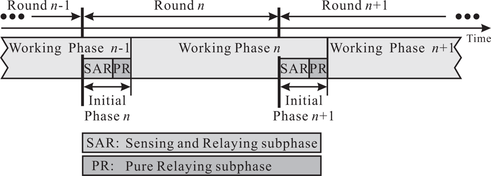
It is well-known that solving ILP is an NP-complete problem. Therefore, two distributed schemes, named REFS (remaining energy first scheme) and EEFS (energy efficiency first scheme), are proposed to solve the MU-CTC problem. As shown in
Figure 2, time is divided into rounds of equal length. A round consists of an
initial phase and a
working phase. The initial phase is further divided into a
sensing and relaying (SAR) subphase and a
pure relaying (PR) subphase. Let
Init,
SAR, and
PR denote the durations of the initial phase, the SAR subphase and the PR subphase, respectively. Clearly,
Init =
SAR +
PR. Note that
Init is much shorter than the duration of a round.
During SAR, each sensor will determine which of its sensing units should be turned on. If the sensor needs to turn on some sensing units, it still needs to find an appropriate neighbor to relay the sensed data. Similarly, the relay node also needs to find its relay node to continue relaying the sensed data to the sink. Basically, whether a sensor needs to be activated and which of its sensing units need to be turned on will be decided during SAR. Consequently, PR is only for the sensor chosen as the relay to find its relay to the sink. The working phase begins at the end of the initial phase and ends at the end of the initial phase of the next round so that the targets can be continually monitored. In addition, in both REFS and EEFS, each sensor makes the decision only by one-hop neighbor information, such as the location, the remaining energy, and the sensing capability of neighbors, as well as the requests for relaying.
4.1. A Generic Approach to the MU-CTC Problem
Algorithm 1 is a generic approach to the MU-CTC problem, which is performed by each sensor during every initial phase in a distributed fashion. Initially, in Step 1, each sensor will set a waiting time, say
Wn for sensor
sn, in order to receive the neighbors’s decision and then make its own decision after
Wn expires. It is worth mentioning that
Wn heavily impacts the performance of the proposed schemes. As a result, in designing
Wn, REFS takes the sensor’s remaining energy into account so that the sensor with more remaining energy can make the decision sooner to take the coverage burden. On the other hand, in EEFS, both the coverage and connectivity are taken into account to efficiently utilize the sensing and communication units of its neighbors’ and its own.
Algorithm 1:.
A generic approach to the MU-CTC problem
Algorithm 1:.
A generic approach to the MU-CTC problem
![Sensors 09 05173i1]() |
In Step 2, each sensor counts down
Wn and waits for the neighbors’ decision until
Wn expires. After
Wn expires, the sensor can decide which sensing and communication units need to be turned on. Therefore, in Step 3, some strategies are adopted to remove the redundant sensing responsibilities or to make the sensing responsibilities more efficiently performed. In Step 4, the relay selection is performed to find an appropriate sensor to relay the sensed data. Finally, in Step 5, the decision, including which sensing units need to be turned on, whether the communication unit needs to be turned on, and which neighbor is selected as the relay, is announced to its neighbors. Based on the generic approach shown in
Algorithm 1, the following two subsections describe the two distributed algorithms, REFS and EEFS, in detail. Notice that the proposed algorithms do not require all sensor to be accurately synchronized. Each sensor only needs to be synchronized with its neighbors. The local synchronization can be achieved through the decision announcement in Step 5.
4.2. Remaining Energy First Scheme (REFS)
REFS is a self-pruning approach, which takes the sensor’s remaining energy and neighbors’ decisions into account to enable its sensing and communication units. Based on
Algorithm 1, the details of REFS are illustrated as follows.
Set Wn
Let
be the sensing capability of the sensing unit
ul on sensor
sn and be defined as
. Furthermore, let Δ
n be the sensing capability of sensor
sn, which is the union of the sensing capabilities of all sensing units equipped on
sn. That is,
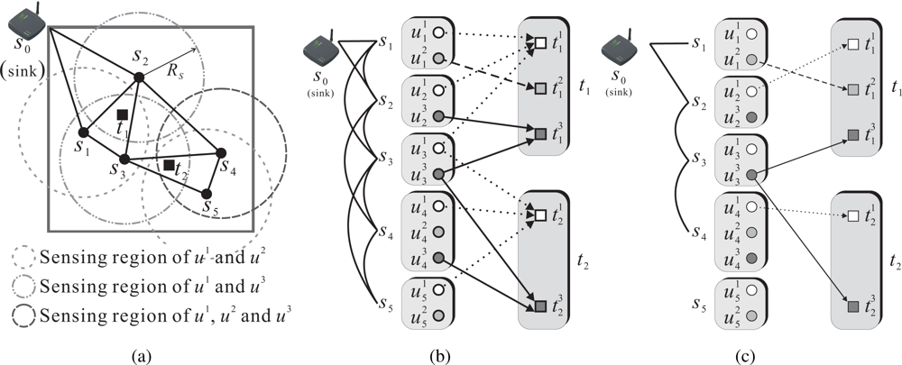
. For the example shown in
Figure 1,
and
. In addition,
and
. Initially, a sensor, say
sn, will take Δ
n as its sensing responsibility. Let Γ
n denote the
sensing responsibility of
sn. Thus, Γ
n is initialized to Δ
n.
In REFS, the setting of
Wn solely depends on the remaining energy of the sensor. The more the energy remains, the shorter is the waiting time. As a result, the sensor with more energy will turn on more sensing units to sense the attributes of the targets. Let
stand for the remaining energy of
sn.
Wn is set as follows:
Countdown Wn
At the beginning of every initial phase, each sensor, say sn, will wait for a waiting time of its own (Wn) and overhear the decisions of the neighbors with smaller waiting time. While receiving the neighbors’ decision packets, the sensor will prune away from Γn those
indicated in the neighbors’ decision packets. Note that, in the neighbors’ decision packets, the next relay is also included. If sn is indicated as a relay, sn should turn on its communication unit and also need to find the next relay for itself in order to relay the sensed data for the neighbors.
Remove incapable sensing responsibilities
After
Wn expires, the remaining Γ
n is the sensing responsibility of
sn at this round. However, it is possible that all remaining energy of
sn is still not enough to support all sensing units indicated in Γ
n. As a result,
sn will orderly remove the sensing units whose sensing capability is the least. If
S is a set, |
S| means the cardinality of
S. Therefore, the deletion of Γ
n can be formally represented as follows.
Finally, sn enables the corresponding sensing units indicated in the remaining Γn to cover the attributes for the indicated targets.
Select the relay
Upon deciding to turn on the sensing units or being indicated as other’s relay,
sn will select a neighbor
sn′ to relay the sensed data to the sink. In general, the sensors closest to the sink are the best. Let
nextRelay(
n) denote the relay sensor for
sn. Therefore, in REFS,
nextRelay(
n) is set as below.
Note that the way to find the relay is the same as geographic routing. However, in geographic routing, a local minimum (dead end) problem will occur. Many approaches have been proposed to handle the problem [
22,
23]. Therefore, the paper does not address the problem. In addition, if
sn does not have enough energy to enable any sensing unit, it will quit executing REFS and turn off all sensing units. The remaining energy of
sn will be left for communication only.
Broadcast my decision
Finally, sn announces its decision as well as the selected relay.
Summary
Overall, REFS is a simple scheme that can be easily implemented. Moreover, REFS incurs less control overhead. However, REFS only takes the sensor’s remaining energy and the neighbors’ decisions into account for making its own decision. The degree of contributions of the sensing units and the communication unit are not considered in REFS. Therefore, the sensor’s energy can not be efficiently utilized. As a result, the sensor applying REFS has a high possibility to enable more redundant sensing or communication units. Consequently, the network lifetime can not be prolonged effectively.
4.3. Energy Efficiency First Scheme (EEFS)
Similar to REFS, EEFS is also a self-pruning approach and is operated at every initial phase by each sensor to individually schedule the on/off state of the sensing and communication units for the following working phase. However, in addition to remaining energy, EEFS also takes coverage and connectivity into consideration. EEFS adds more heuristics to prune the redundant or inefficient sensing responsibilities away and select the relay intelligently.
Before executing EEFS, each sensor has to collect its neighbors’ sensing capabilities and critical sensing responsibilities in advance in order to make the most efficient use of its sensing and communication units. The
critical sensing responsibility of a sensor is the attributes of the targets (in terms of
) that can be sensed only by that sensor. Let Θ
n be the critical sensing responsibility of
sn.
. For the example shown in
Figure 1,
. In other words, each sensor, say
sn, has to compute Δ
n and Θ
n as well as collect Δ
n′ and Θ
n′,
∀ n′ ∈ ℵ(
n), in advance. Nevertheless, the collection needs to be performed only once. Moreover, to balance the energy consumption and efficiently utilize the energy of sensors, each sensor has to exchange
with its neighbors at the beginning of EEFS. Based on
Algorithm 1, the details of EEFS are described as follows.
Set Wn
In EEFS, sensor sn calculates Wn by the following information: (1) the sensing capabilities, (2) the critical sensing responsibilities, (3) the remaining energy of itself and its neighbors, as well as (4) the probability of being others’ relay. According to the sensing capabilities as well as the critical sensing responsibilities of itself and its neighbors, sensor sn will rank its sensing priority among its neighbors. The sensor with higher sensing priority and lower probability of being others’ relay has shorter Wn so that the sensor can make its decision sooner. A sensor’s sensing priority and the probability of being others’ relay are regarded as its coverage contribution and connectivity contribution, respectively.
Coverage contribution
The coverage contribution of a sensor reflects the ranking of the sensor among its neighbors in regard to the sensing capability. The ranking is processed as follows. If sn is equipped with the sensing unit ul, sn will sort the sensing capability of
in an increasing order to a list l according to
. If the sensing capabilities of two sensors are the same, the higher priority will be assigned to the one with more remaining energy. Otherwise, the sensor with a larger ID wins. Notice that only the sensor equipped with ul is included in the ranking process. Let
be the order in l, which represents the priority of the sensing unit ul of sn among its neighbors. The larger the
is, the higher its priority is. It is worth mentioning that the reason to take a rank among the neighbors is to normalize the
for different ul on sn.
Take
s1 in
Figure 1 as an example. Since
ℵ(
s1) = {
s2,
s3}, only
s1,
s2, and
s3 are taken into account. Suppose
E = 8,
,
, and
. Since
s1 is equipped with
u1 and
u2,
and
as well as
and
are to be calculated, where
. Firstly,
u1 is considered. Obviously,
,
, and
. Since
, the remaining energy is taken into account. Therefore, the priority of
among
s1 and its neighbors is:
. That is,
. Consequently,
and
. With regard to
u2, since
s2 and
s3 are not equipped with
u2, therefore,
and
.
Let
ρn be the priority of
sn, which takes the priorities of all sensing units equipped on
sn into consideration.
ρn is set as:
For the above example,
.
Because the number of sensing units equipped on sensors is different, the coverage contribution of
sn, denoted
ρ̄n, is defined as the average priority of the sensing units equipped on
sn and represented as follows.
Notice that 0 <
ρ̄n ≤ 1. With regard to the example in
Figure 1,
.
Connectivity contribution
The connectivity contribution of a sensor is defined as the probability of being others’ relay. Let σn be the connectivity contribution of sn. σn is determined as follows.
It is hard for a sensor to find the best route to the sink merely by its local information, such as the one-hop neighbor information. Like REFS, the neighbor with the shortest distance to the sink is the best candidate to relay the sensed data for the sensor. Therefore, a sensor closest to the sink has a higher probability to serve as others’ relay. Based on the concept, the location of the relay for sensor
sn can only be located in the
forwarding zone of
sn. The definition of the forwarding zone of
sn is defined as follows, where
C(
s, R) denotes a circle centered at
s with the radius
R.
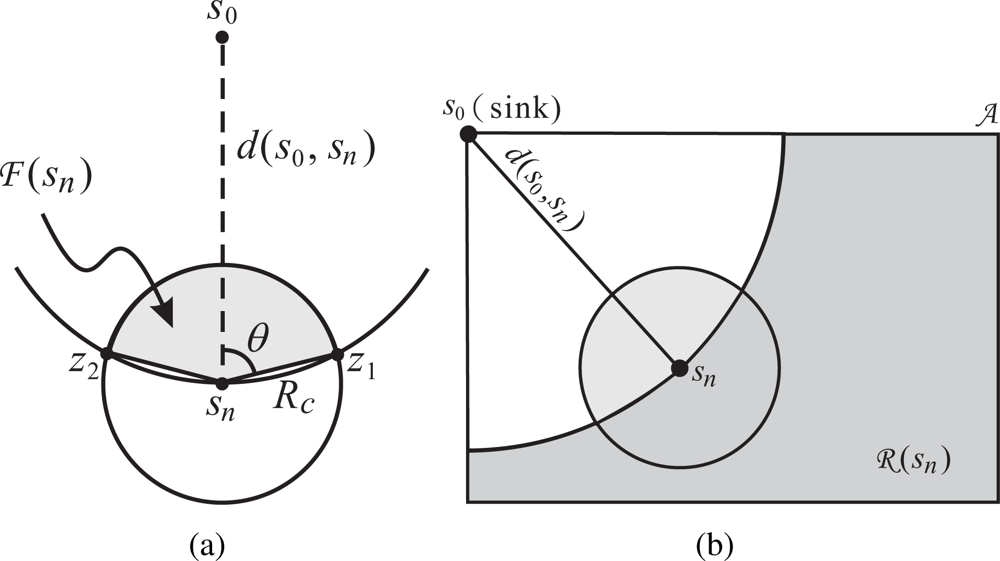
Figure 3 (a) also illustrates the forwarding zone of
sn.
Definition 3 (Forwarding Zone) Let the intersection points of two circles C(s0, d(s0, sn)) and C(sn, Rc) be z1 and z2. The forwarding zone of sn, denoted (sn), is defined as the circular sector formed by two radii and, and the arc.
Compared with
sn, the sensor located in the forwarding zone of
sn has a shorter to-sink-distance, which is defined as the distance from the sensor to the sink. On the contrary, the sensor located in the area
C(
sn,
Rc)
− (
sn) has a longer to-sink-distance than
sn. It implies that the sensor located in
C(
sn,
Rc)
− (
sn) may choose
sn as its relay. Consequently, the more the sensors are located in
C(
sn,
Rc)
− (
sn), the more likely
sn become others’ relay. Therefore,
The higher the
σn is, the more likely
sn become others’ relay. Similarly, consider the same example in
Figure 1. Because
s2 and the sink, regarded as a neighbor of
s1, are located at (
s1),
.
The setting of Wn
A sensor with a higher coverage contribution can more efficiently cover the targets, that is, consume less energy but cover more targets. Therefore, the sensor with a higher coverage contribution shall make its decision sooner, implying a shorter Wn. On the other hand, a sensor with a higher connectivity contribution has a higher probability to relay. If the sensor is selected as a relay, a longer waiting time can let it make its decision later, to be likely to turn on its sensing units to cover the targets, and balance its energy consumption. Consequently, the sensor with a higher connectivity contribution shall wait for a longer time to make its decision.
As a result, a sensor with a higher coverage contribution and a lower connectivity contribution will have a shorter
Wn so that the sensor can determine whether it should turn on its sensing and/or communication units.
Wn is set as follows.
where
αn is the
contribution tendency of
sn on coverage contribution or connectivity contribution. Basically, a sensor near the sink may have a higher probability to forward others the sensed data, because all the sensed data should be forwarded to the sink. The sensor near the sink shall have a higher connectivity tendency to relay the sensed data in order to keep the network connected. On the other hand, a sensor covering more targets shall have a higher coverage contribution tendency to sense the targets. Therefore, each sensor in the sensing field shall have different
αn to make the best use of its contribution tendency. In other words, in addition to the status of neighbors, the hardware difference and the location of a sensor should be considered to determine
Wn. How to determine each sensors’
αn will be shown in detail in next subsection.
In order to demonstrate how the coverage and connectivity contributions affects
Wn, assume that the
αn of the sensors in the example in
Figure 1 are the same and set to 0.5. That is, the locations and the energy model of the sensors in
Figure 1 is assumed similar. According to
Equation (2),
. Similarly,
W2 can be calculated as follows. Assume
,
. On the other hand, because only the sink is located in (
s2),
. Therefore,
. Clearly,
s1 will make its decision first, because
W1 <
W2. In
Figure 1, both
s1 and
s2 are equipped with two kinds of sensing units that can sense the corresponding sensing attributes at
t1. Therefore,
s1 and
s2 have approximately the same coverage contribution. However, because the number of
s2’s neighbors is more than that of
s1,
s2 should make its decision later to ensure the network connectivity.
The setting of αn
The tendency of a sensor toward coverage or connectivity is determined according to the locations of the targets, which are known by all sensors in advance. If the amount of sensed data to be relayed by a sensor is large, the sensor will take a higher priority in relaying the sensed data, instead of sensing the targets. Therefore, a
relaying zone of a sensor is defined to estimate the amount of sensed data to be relayed by the sensor. Let
(
sn) denote the
relaying zone of
sn. Definition 4 and
Figure 3(b) give the formal definition and an illustration of
(
sn), respectively.
Definition 4 (Relaying Zone) Let (
sn)
denote the relaying zone of sn.
It is possible that the sensed data from the targets located in
(
sn) may need
sn to relay to the sink. Therefore, the number of targets located in
(
sn) can be regarded as the amount of sensed data which needs
sn to relay to the sink. As a result, a sensor with a larger number of targets in
(
sn) shall have a higher connectivity contribution tendency. Formally,
αn of
sn is set as follows.
where ɛ is a system adjustable parameter to reflect the hardware difference. If the energy cost of the communication unit is much higher than that of the sensing unit, even if the sensor has a higher priority in coverage contribution, the sensor should still pay more attention on the connectivity contribution. In contrast, if the energy cost of the sensing unit is higher than that of the communication unit, the sensor should put a higher weight on coverage contribution, regardless of the distance from the sensor to the sink. Therefore, ɛ is set high when the energy cost of the sensing unit is lower than that of the communication unit. Otherwise, ɛ is set low accordingly. Basically, ɛ is set between 0 and 1.
Notice that αn is based on the hardware characteristic, e.g., the energy consumption models of sensing and communication units, and the environment characteristic, e.g., the locations of sensors. These characteristics have an influence on whether a sensor can spend its energy efficiently on sensing or communication. However, these characteristics of a sensor are unchanged after the sensor is deployed. Therefore, it is not sufficient for the sensor to efficiently use its energy. When determining Wn, a sensor also has to locally take the coverage and connectivity contributions among its neighbors and itself, as well as the remaining energy into consideration to meet the sensing requirements, to ensure the network connectivity, and to prolong the network lifetime.
Countdown Wn
The processes to be performed here are the same as those in Step 2 of REFS.
Remove incapable or redundant sensing responsibilities
Upon the expiration of Wn, the remaining Γn is the sensing responsibility of sn in this round. However, it is still possible for sn to alleviate its burden via pruning out redundant sensing responsibilities. For example, for some neighbor of sn, say sn′, if Θn′ ≠ ∅, sn′ has the responsibility to cover the sensing responsibilities indicated in Θn′. Suppose sn′ turns on ul, for some l, to cover
, for some m. If turning on the sensing unit ul also covers the other targets, say
, for some m′ (that is,
) and
, therefore,
can be pruned awat from Γn. As a result, Γn can be further improved.
In addition, it is possible to improve by pruning the inefficient sensing responsibilities of
sn if it is better to leave these responsibilities to the neighbors with higher sensing efficiency. As defined above,
is the sensing capability of
. The more
is, the more targets
can cover at a time. Therefore,
can be regarded as the
benefit of
if
is turned on. On the contrary,
can be regarded as the
cost of
, where
el and
are the energy consumption of
ul in sensing for a time unit and the remaining energy of
sn, respectively. The cost considers not only the energy consumption of
ul, but also takes the remaining energy of
sn into account in order to reflect the effect of the energy consumption of
ul on the remaining energy of
sn. Consequently,
can be regarded as the
benefit-cost ratio (BCR) of
. In addition to the BCR of
, the sensing efficiency of
on
sn should take the ratio of the remaining energy of
sn to the initial energy into consideration as well. Therefore, let
and
Eff(
sn,
ul) denote the BCR of
and the sensing efficiency of
ul on
sn, respectively. Accordingly, the sensing efficiency of
ul on
sn,
Eff(
sn,
ul), is defined as below.
In designing Eff(sn, ul), the contribution tendency is also considered to differentiate the sensors nearby or far away from the sink with the same sensing unit to increase the sensing efficiency. To do so can further alleviate the sensing responsibility of sn. As a result, if there exists a sensor, say sn′, who has not sent out the DecAnn packet and whose sensing efficiency of ul is better than that of ul on sn, then sn will leave the sensing responsibilities covered by ul to sn′.
Select the relay
In EEFS, in addition to the neighbor’s to-sink-distance, the remaining energy of the neighbor is also taken into account for
sn to select its relay. Basically, the neighbor with more remaining energy and shorter to-sink-distance will be selected as a relay. However, it is possible that the neighbor with a longer to-sink-distance may be selected. This will result in a longer path to the sink. Therefore, in EEFS, the neighbors located in
(
sn) are considered as relay candidates, instead of all the neighbors. Formally,
nextRelay(
n) is set as below.
where
and
are to normalize the to-sink-distance and the remaining energy of
sn′, respectively. Notice that the case of |
(
sn)|= 0 is regarded as the local minimum problem and is not addressed in the paper.
Broadcast my decision
sn announces its decision by sending out a DecAnn packet.
Summary
As mentioned above, REFS has a significant drawback that a sensor may turn on too many redundant sensing units. It is because a sensor in REFS only considers its remaining energy and its neighbors’ decisions. However, EEFS can alleviate such a situation and make the best use of the sensing and communication units equipped on a sensor. In addition, the coverage and connectivity contributions are introduced in designing Wn of sn. To do so can let the sensor make its decision sooner if it has a higher sensing capability and a lower probability to relay for others. The order of making a decision has a significant impact on the performance of both REFS and EEFS. Moreover, in EEFS, both the coverage and the connectivity contributions are taken into account. As a result, a sensor with a better coverage or connectivity contribution can make its best decision either in covering the target or in relaying the sensed data. Consequently, the network lifetime can be prolonged efficiently.
The complete REFS and EEFS algorithms are omitted due to the space limitation.
5. Performance Evaluations
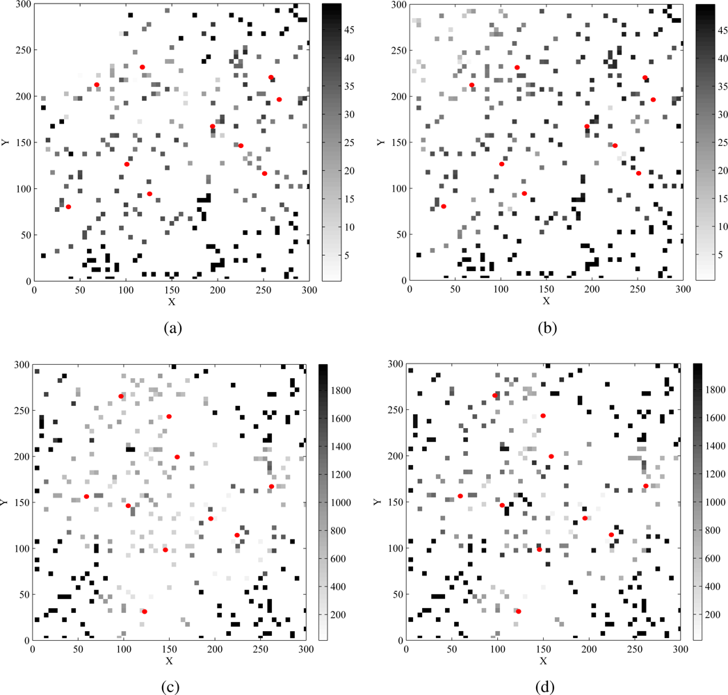
In this section, scheduling multiple sensing units on each sensor to sense a given number of targets and relay the sensed data to the sink in a WHSN are simulated extensively. The simulation setting for the MU-CTC problem is summarized in
Table 2. The numbers of sensors and targets are specified in each simulation. The number and types of sensing units on sensors are also specified in each simulation, whereas the number and types of sensing units on each sensor are randomly selected. Similarly, the number and types of attributes required to be sensed at each target are all randomly selected as well. Moreover, targets and sensors are randomly deployed in the sensing field. The locations of sensors and targets are fixed during the whole simulation. The sensing range of each sensing unit is the same and is set as 50 m. The communication range of each sensor is twice of the sensing range. A reliable communication channel is assumed in these simulations. All measurements are averaged over 10 runs, if not otherwise specified.
Since the ILP solution is a centralized scheme, no control and computation overheads are counted. Therefore, two different scenarios are considered. In the first scenario, REFS and EEFS are compared with the ILP solution to show the efficiency of the proposed schemes without the control and computation overheads, where the ILP solution is implemented by ILOG CPLEX [
24] optimization library. In the second scenario, REFS and EEFS are evaluated when the control and computation overheads are considered. In order to show the effectiveness of the proposed algorithms, a straightforward scheme, named
m-SU-CTC, is compared in this scenario. As mentioned above, there existed several schemes in the literature considering the CTC problem on a wireless homogeneous sensor network, where each sensor is equipped with only one sensing unit and only one attribute is required to be sensed at each target. Therefore, the
m-SU-CTC will apply this kind of scheme multiple times, each for the required attribute to be sensed at the targets, so that all the attributes required to be sensed by every target are sensed by the sensors with those specific sensing units on sensors.
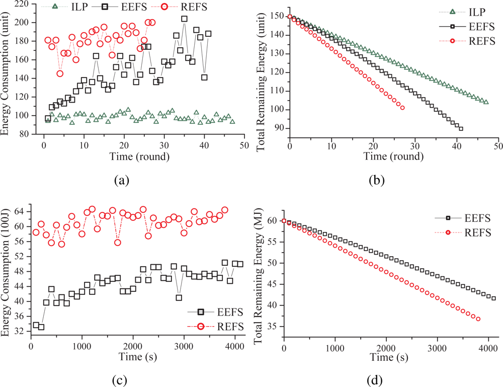
Energy consumption and network lifetime are mainly evaluated to verify the performance of the proposed schemes. As mentioned above, the network lifetime is defined as the time interval from the beginning to the time that either the attributes required to be sensed at any target can not be sensed anymore or the sensed data can not be delivered to the sink. On the other hand, the energy consumption models for sensing, communication, and computation are different in scenarios 1 and 2. In scenario 1, the initial energy of each sensor is 50 units. The energy consumption of each type of sensing unit is assumed linearly proportional to the type of the sensing unit. That is, the first type of the sensing unit is assumed to consume one unit of energy in a round, the second type of the sensing unit consumes two units of energy, and likewise. Additionally, the communication module of a sensor consumes one unit of energy to send or receive a unit of the sensed data.
In scenario 2, the energy consumption caused by control and computation overheads are considered. The energy consumption model of MICA2 [
4] is adopted in the simulation. In addition, the initial energy of each sensor is assumed 2000
J. A sensor in active mode consumes 10.9
mA. Similar to scenario 1, the energy consumption of each type of the sensing unit is also assumed linearly proportional to the type of the sensing unit. However, the unit of the energy consumption of the sensing units is
J/min. If a sensor decides to turn on any sensing unit, the sensor is assumed to reply the sensed data to the sink every 10 minutes. Each round is 100 minutes.
Table 3 summaries the energy consumption model used in scenario 2.
Since there is a system parameter ɛ involved in the design of the EEFS in order to obtain an appropriate value of ɛ for scenarios 1 and 2, the experiment contains two parts. The first part is to observe the impact of ɛ on the performance of EEFS for scenarios 1 and 2. According to the results obtained from the first part, the second part of the experiment evaluates the performance of the proposed schemes. As mentioned above, scenario 1 compares the performance of the proposed schemes, REFS and EEFS, against the ILP solution, where the control and computation overheads are not taken into account. In scenario 2, the proposed schemes are compared against a heuristic scheme, where the control and computation overheads are considered.
5.1. The Impact of ɛ
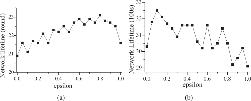
In EEFS, ɛ is a system parameter considering the difference of the energy consumption between the communication unit and the sensing units. The use of the ɛ is to make the best use of the sensing and communication units and increase the network lifetime. Therefore, this part of experiment focuses on the impacts of ɛ on the network lifetime for scenarios 1 and 2. In this experiment, three types of attributes are required to be sensed and there are 25 targets and 300 sensors randomly deployed in the 300 m * 300 m sensing field.
Figures 4(a) and
4(b) show the results for scenarios 1 and 2, respectively. According to
Figure 4(a), basically, the network lifetime increases with the increase of ɛ until ɛ = 0.8. The best performance is observed when ɛ = 0.8. In scenario 1, the energy spent in sensing is close to that spent in communication, which implies that the cost of the communication unit is higher than that of the sensing unit. As mentioned above, the sensor should pay more attention on the connectivity contribution. Consequently, ɛ should be set high, which is also coincident with the simulation results shown in
Figure 4(a). Note that, in scenario 1, the control overhead is not taken into account. However, if the control overhead is taken into consideration, ɛ should be larger than 0.8.
On the other hand, in scenario 2, the energy cost of the sensing unit is much higher than that of the communication unit. Therefore, the sensor should have a higher tendency toward the coverage contribution. As a result, ɛ should be set low to have the sensor toward the coverage tendency. According to
Figure 4(b), the network lifetime decreases with the increase of ɛ. The network obtains the longest lifetime when ɛ = 0.1. Consequently, for the following simulations, ɛ are set to 0.8 and 0.1 for scenarios 1 and 2, respectively.
5.3. Summary
The simulation results can be summarized as follows.
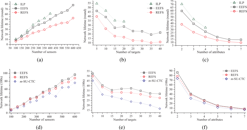
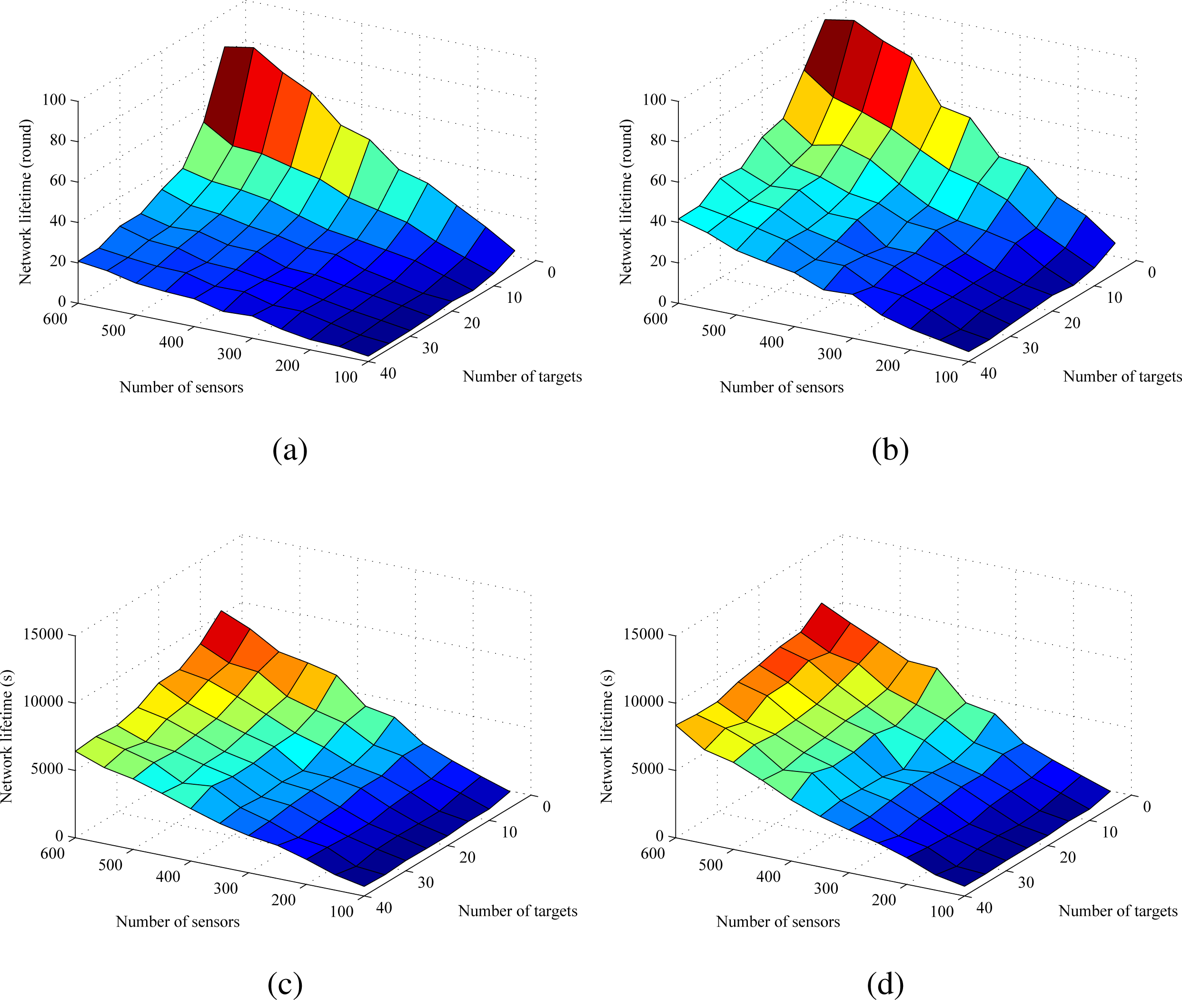
The network lifetime increases with the increase of the number of sensors.
The network lifetime decreases with the increase of the number of targets.
The network lifetime decreases with the increase of the number of attributes.
The performance of EEFS is very close to that of the ILP solution, which is an optimal solution.
According to the simulation results, even though the control overhead of EEFS is higher than that of REFS, the performance of EEFS is still better than that of REFS. However, since the computation cost of EEFS is higher than that of REFS, if the computation capability of a sensor is not good enough, REFS may be a better choice.
The modified algorithm m-SU-CTC originally designed for the sensor with one sensing unit may not work well in WHSNs because m-SU-CTC does not jointly take the sensing abilities of the equipped sensing units into consideration.
Even though the ILP solution performs the best, REFS and EEFS are still the practical solutions to WHSNs.
6. Conclusions
Coverage and connectivity are important measurements for the quality of surveillance that a sensor network can provide. Therefore, the paper emphasizes on the connected target coverage problem in wireless heterogeneous sensor networks with multiple sensing units, termed the MU-CTC (Multiple sensing Units for Connected Target Coverage) problem. The problem is to schedule the activity of each sensing unit on each sensor to completely cover the targets of interest, to make sensors relay the sensed data to the sink, and, subject to the energy constraint of each sensor, to maximize the network lifetime. The problem is further reduced to a connected set cover problem, called the MU-CSC (Multiple sensing Units for Connected Set Cover) problem. According to the MU-CSC problem, several ILP constraints are proposed. In addition, two distributed schemes, REFS and EEFS, are proposed to solve the MU-CTC problem. These two schemes are executed by each sensor in the initial phase of each round. In REFS, each sensor enables its sensing units by its remaining energy and neighbors’ decisions. However, in EEFS, the coverage and connectivity contributions are also taken into account. Simulation results show that REFS and EEFS can prolong the network lifetime effectively. The performances of the two schemes are close to that of the ILP solution. However, the ILP solution is a centralized and computationally intensive scheme, so the proposed distributed schemes are much more practical. In addition, the schemes can be easily implemented in a real network.
In the future, different levels of target coverage requirements (e.g., k-coverage) will also be considered to meet the sensing requirements of different applications. From the practical viewpoint, the sensing units with different sensing ranges will also be taken into consideration in the future.


