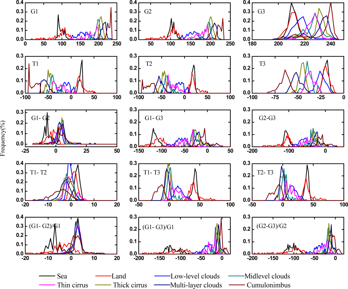
Figure 1.
The frequency distribution of features of FY-2C cloud samples.
Figure 1.
The frequency distribution of features of FY-2C cloud samples.
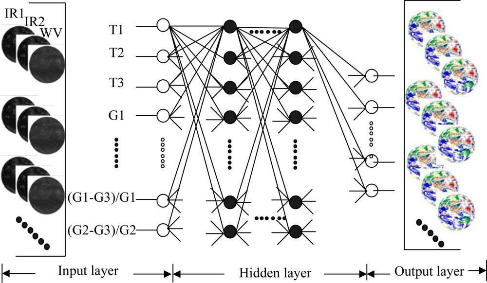
Figure 2.
Configuration for the cloud classification: on the lefts are the input satellite images; at the middle are features extracted by GLCM and configuration of classifier; and on the rights are the output cloud classification results. Note white circles on the left are input neurons, and in the right are output ones. Black circles are neurons in hidden layer. Lines around circles show the data flow.
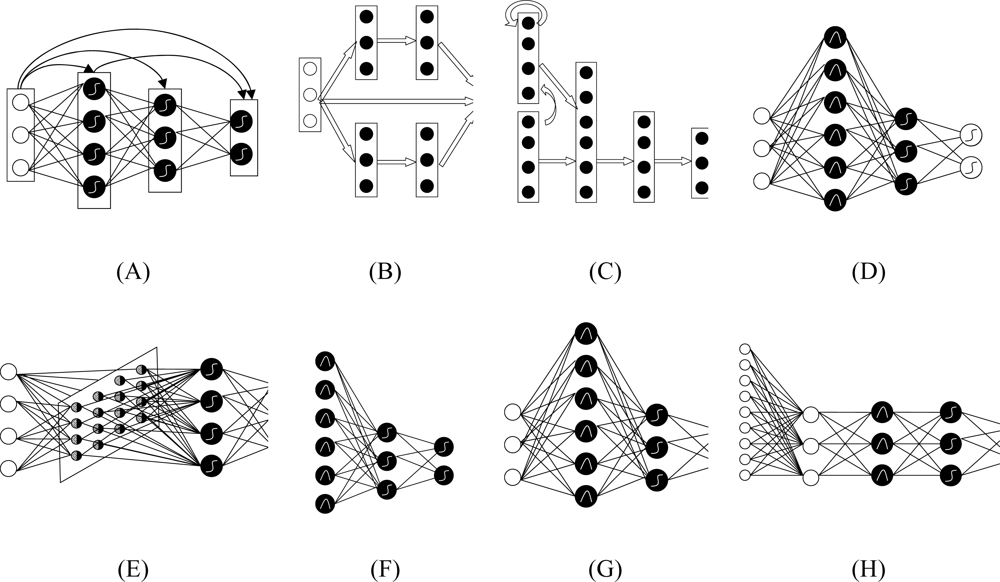
Figure 3.
Schematic diagram of eight cloud classifiers: in general the left layer is input layer; the right layer is output layer; and the middle ones are hidden layers. Note that the white circles in the left are input neurons, and in the right are output ones. Black circles are neurons in hidden layer. Lines around circles and arrows between layers show the data flow between neuron and layers respectively. Curves in circles show the transfer function. The linear sum, sigmoid function and Gaussian function are three often used functions. (A) Back Propagation (BP): Its connections can jump over one or more layers. (B) Modular Neural Networks (MNN): It uses several parallel MLPs, and then recombines the results. (C) Jordan-Elman network: It extends the multilayer perceptron with context units, which are processing elements (PEs) that remember past activity. (D) Probabilistic Neural Network (PNN): It uses Gaussian transfer functions and all the weights can be calculated analytically. (E) Self-Organizing Map (SOM): It transforms the input of arbitrary dimension into a one or two dimensional discrete map subject to a topological constraint. (F) Co-Active Neuro-Fuzzy Inference System (CANFIS): It integrates adaptable fuzzy inputs with a modular neural network to rapidly and accurately approximate complex functions. (G) Support Vector Machine (SVM): It uses the kernel Adatron to change inputs to a high-dimensional feature space, and then optimally separates data into their respective classes by isolating those inputs which fall close to the data boundaries. (H) Principal Component Analysis (PCA): It is an unsupervised linear procedure that finds a set of uncorrelated features, principal components, from the input.
![Sensors 09 05558f3]()
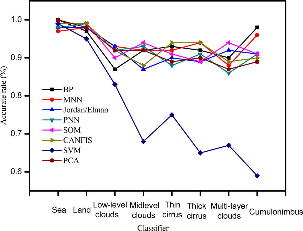
Figure 4.
The accuracy rate of the eight cloud classifiers for the test data.
Figure 4.
The accuracy rate of the eight cloud classifiers for the test data.
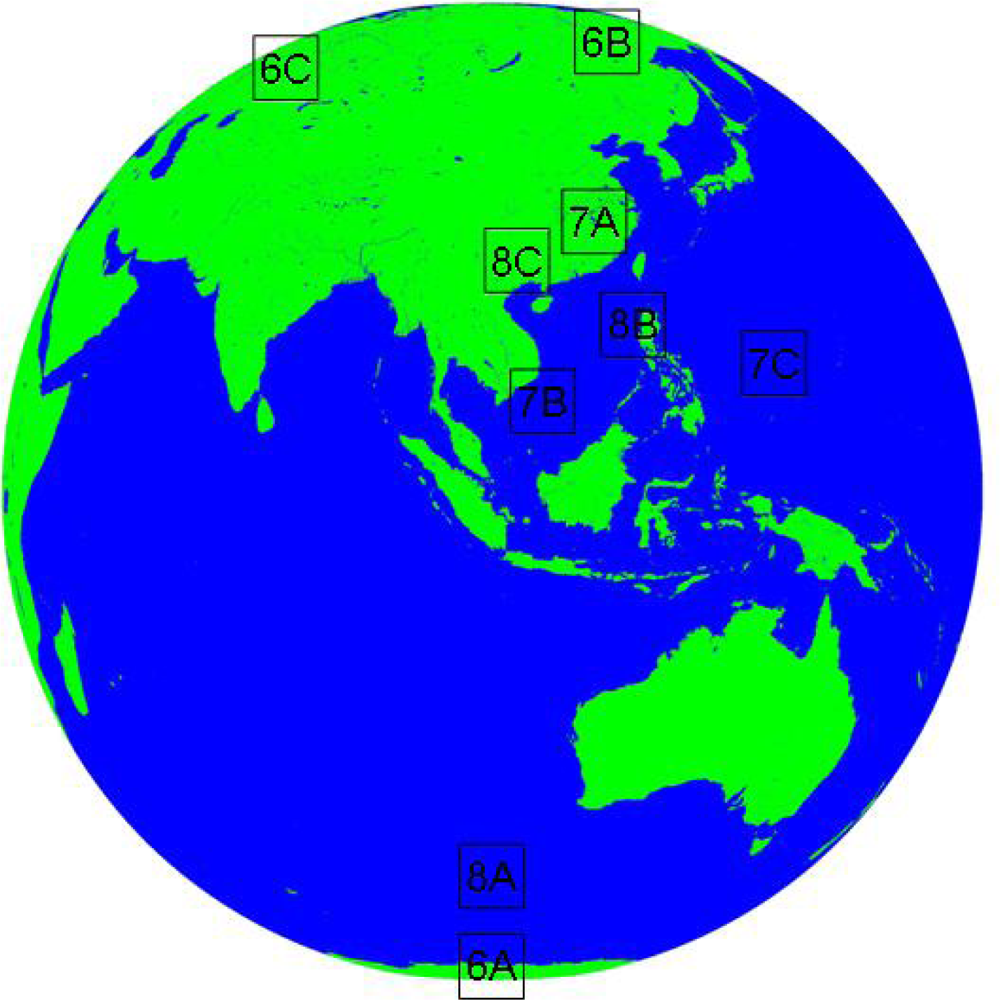
Figure 5.
Location of cases: 6X (6A, 6B,6C) is the location of case A, B, C in high latitude (
Figure 6); 7X (7A, 7B,7C) is the location of case A, B, C of Cumulonimbus (
Figure 7); and 8X (8A, 8B, 8C) is the location of case A, B, C of cirrus (
Figure 8).
Figure 5.
Location of cases: 6X (6A, 6B,6C) is the location of case A, B, C in high latitude (
Figure 6); 7X (7A, 7B,7C) is the location of case A, B, C of Cumulonimbus (
Figure 7); and 8X (8A, 8B, 8C) is the location of case A, B, C of cirrus (
Figure 8).
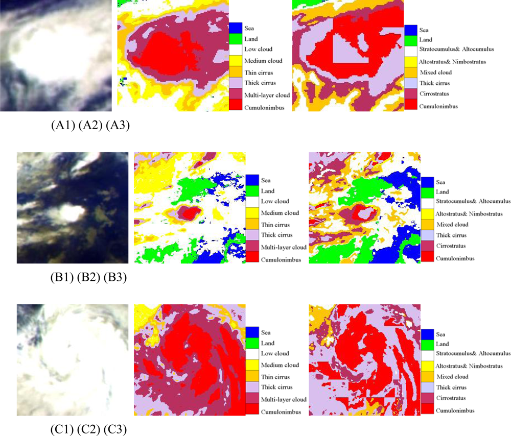
Figure 6.
(A) The first line (A1, A2, A3) are high latitude cases at 07: 00 UTC (daytime); (B) The second line (B1, B2, B3) are high latitude cases at 15: 00 UTC (night); (C) the third line (C1, C2, C3) are high latitude cases at 23: 00 UTC (twilight); The first column (A1, B1, C1) are false RGB composite of Tbb of IR1, IR2 and WV; The second column (A2, B2, C2) are cloud classification results of ANN; The third column (A3, B3, C3) are results of FY-2C operational products.
Figure 7.
(A) The first line (A1, A2, A3) are cumulonimbus cases at 07: 00 UTC (daytime); (B) The second line (B1, B2, B3) are cumulonimbus(Cb) cases at 15: 00 UTC (night); (C) the third line (C1, C2, C3) are cumulonimbus(Cb) cases at 23: 00 UTC (twilight); The first column (A1, B1, C1) are pseudo-color composite map of Tbb of IR1, IR2 and WV; The second column (A2, B2, C2) are cloud classification results of ANN; The third column (A3, B3, C3) are results of FY-2C operational products.
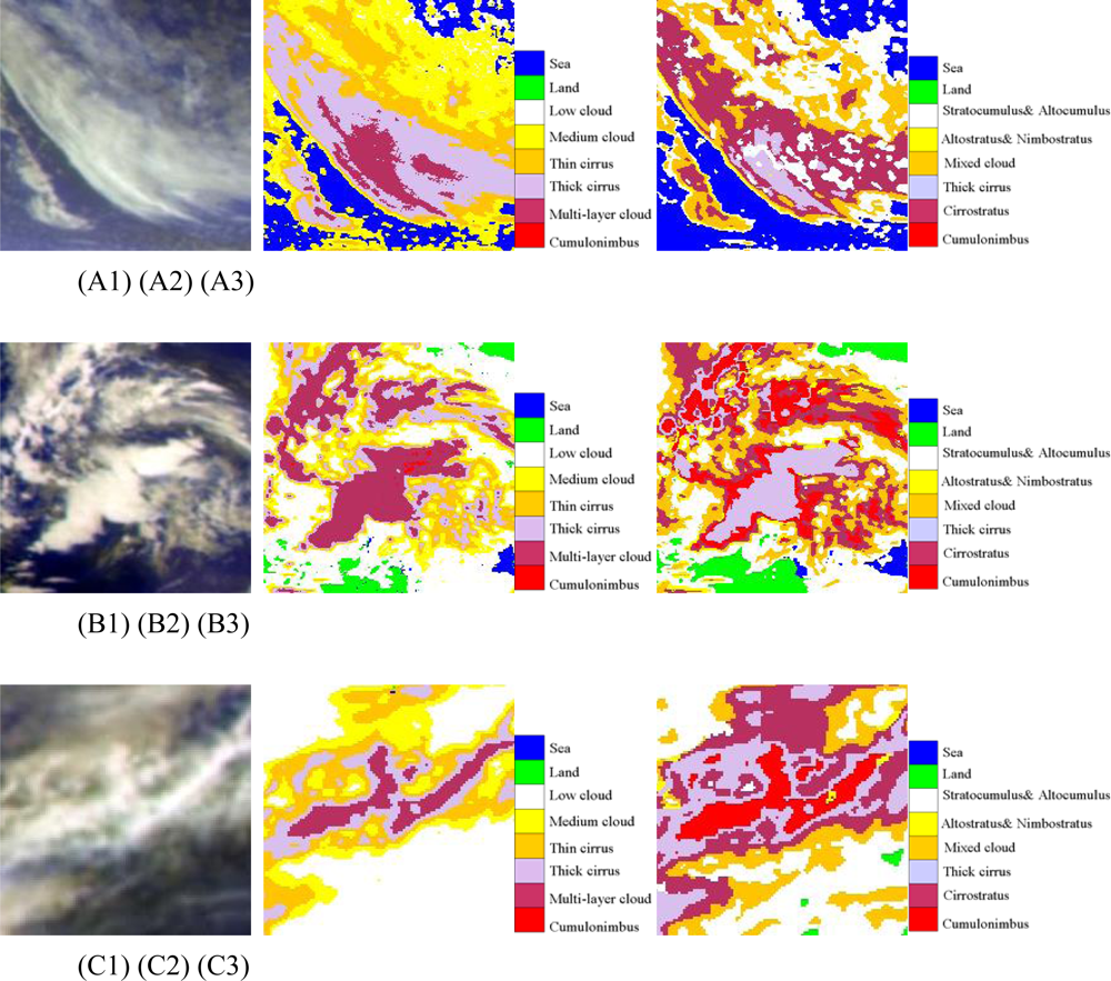
Figure 8.
(A) The first line (A1, A2, A3) are cirrus at 07: 00 UTC(daytime); (B) The second line (B1, B2, B3) are cirrus cases at 15: 00 UTC (night); (C) the third line (C1, C2, C3) are cirrus cases at 23: 00 UTC (twilight); The first column (A1, B1, C1) are pseudo-color composite map of Tbb of IR1, IR2 and WV; The second column (A2, B2, C2) are cloud classification results of ANN; The third column (A3, B3, C3) are results of the FY-2C operational product.
Table 1.
Specifications of VISSR channels: spectral range and spatial resolutions.
Table 1.
Specifications of VISSR channels: spectral range and spatial resolutions.
| Channel No. | Channel name | Spectral range (μm) | Spatial resolution (km) |
|---|
| 1 | IR1 | 10.3–11.3 | 5 |
| 2 | IR2 | 11.5–12.5 | 5 |
| 3 | IR3(WV) | 6.3–7.6 | 5 |
| 4 | IR4 | 3.5–4.0 | 5 |
| 5 | VIS | 0.55–0.90 | 1.25 |
Table 2.
The set of classes and samples in this study.
Table 2.
The set of classes and samples in this study.
| Classes | Samples | Description |
|---|
| Sea | 184 | Clear sea |
| Land | 266 | Clear land |
| Low-level clouds | 405 | Stratocumulus (Sc), Cumulus (Cu), Stratus (St), Fog, and Fractostratus (Fs) |
| Midlevel clouds | 379 | Altocumulus (Ac), Altostratus (As), and Towering Cumulus |
| Thin cirrus | 415 | Thin cirrus |
| Thick cirrus | 440 | Thick cirrus |
| Multi-layer clouds | 371 | Cumulus congestus (Cu con), Cirrostratus (Cs) and Cirrocumulus (Cc) |
| Cumulonimbus | 404 | Cumulonimbus(Cb) |
| Sum | 2864 | |
Table 3.
Selected Features according to the Gray Level Co-occurrence Matrices (GLCM) for cloud classification. Note that Ti (T1, T2, T3) is the Tbb of channel i (IR1, IR2 and WV) and Gi (G1, G2, G3) is the gray value of channel i (IR1, IR2 and WV).
Table 3.
Selected Features according to the Gray Level Co-occurrence Matrices (GLCM) for cloud classification. Note that Ti (T1, T2, T3) is the Tbb of channel i (IR1, IR2 and WV) and Gi (G1, G2, G3) is the gray value of channel i (IR1, IR2 and WV).
| Features | Parameters | Description |
|---|
| Spectral features | T1,T2, T3 | Top brightness temperature of IR1,IR2,WV |
| Gray features | G1, G2, G3 | Gray value of IR1,IR2,WV |
| G1–G2, G1–G3, G2–G3 | |
| Assemblage features | T1–T2, T1–T3, T2–T3 | The combination of infra split window and water vapor channel |
| (G1–G2)/G1, (G1–G3)/G1, (G2–G3)/G2 | |
Table 4.
Parameters of eight cloud classifiers
*.
Table 4.
Parameters of eight cloud classifiers*.
| Type of network | Output layer | Hidden layer |
|---|
|
|---|
| Learning step | Number of hidden layer | Number of Neurons | Learning step |
|---|
| ANN | BP | 0.10 | 2 | 9,4**(1) | 0.10 |
| MNN | 0.10 | 1 | 4,4**(2) | 0.10 |
| Jordan/Elman***(1) | 0.10 | 1 | 9 | 0.10 |
| PNN***(2) | 1.00 | 1 | 6 | 1.00 |
| SOM Network***(3) | 0.10 | 1 | 9 | 1.00 |
| CANFIS***(4) | 0.10 | 1 | 4 | 0.10 |
|
| SVM | 0.01 | | | |
|
| PCA***(5) | 0.10 | | | |
Table 5.
The evaluation result of the eight cloud classifiers for the training and testing data.
Table 5.
The evaluation result of the eight cloud classifiers for the training and testing data.
| | Cross-examination (Training) | Test |
|---|
| Method | Time(S) | MSE | NMSE | Corr | Errol (%) | AIC | MDL | MSE | NMSE | Corr | Errol (%) | AIC | MDL |
|---|
| BP | 30.00 | 0.01 | 0.02 | 0.99 | 9.35 | −399.35 | −214.35 | 0.01 | 0.02 | 0.99 | 8.87 | −2693.14 | −3376.66 |
| MNN | 21.00 | 0.02 | 0.05 | 0.98 | 9.20 | −106.53 | −46.16 | 0.01 | 0.03 | 0.99 | 8.87 | −2832.60 | −2599.99 |
| Jordan/Elman | 22.00 | 0.01 | 0.03 | 0.99 | 8.75 | −31.27 | −126.34 | 0.02 | 0.03 | 0.99 | 8.88 | −3852.71 | −3398.99 |
| PNN | 63.00 | 0.01 | 0.03 | 0.99 | 8.52 | 2812.18 | 3428.47 | 0.01 | 0.02 | 0.99 | 7.75 | −20.61 | 2160.85 |
| SOM | 21.00 | 0.03 | 0.05 | 0.98 | 8.92 | 854.12 | 947.30 | 0.01 | 0.02 | 0.99 | 7.74 | −1340.14 | −699.23 |
| CANFIS | 44.00 | 0.02 | 0.04 | 0.98 | 10.53 | 464.56 | 924.43 | 0.02 | 0.03 | 0.99 | 9.23 | −4851.31 | −3776.72 |
| SVM | 22.30 | 0.67 | 2.01 | −0.08 | 49.82 | 38837.55 | 4820.26 | 0.67 | 2.01 | −0.08 | 49.82 | 38837.55 | 48200.26 |
| PCA | 19.00 | 0.02 | 0.03 | 0.99 | 10.42 | −46.33 | −48.75 | 0.01 | 0.02 | 0.99 | 10.18 | −1449.86 | −1293.18 |
Table 6.
Accuracy rate of FY-2C operational product and ANN model (%).
Table 6.
Accuracy rate of FY-2C operational product and ANN model (%).
| Type | FY2C product | ANN cloud classification |
|---|
| Sea | 83.02 | 99.01 |
| Thick Cirrus | 26.14 | 88.79 |
| Cumulonimbus | 76.49 | 90.74 |
| Land | 48.35 | 98.51 |


