Improved Estimation of Protein-Ligand Binding Free Energy by Using the Ligand-Entropy and Mobility of Water Molecules

Abstract
:1. Introduction
2. Results and Discussion
2.1. Original Direct Interaction Approximation (DIA) Method


 could be an unrealistically large value when the denominator of Equation (5) is nearly zero. Thus, we introduce a parameter x and the scale function as follows:

 , was used as the scale factor, and the previous study showed that the optimal value was 0.6 [30]. Note that the actual effective dielectric constant corresponds to /β.
2.2. Intra-Molecular Ligand-Entropy Term

2.3. Hydration Effect of Each Residue of the Target Protein


 > and <
  > was 0.32. The average (Cavg), minimum and maximum < > values were 73.51, 0, and 106.2, respectively.
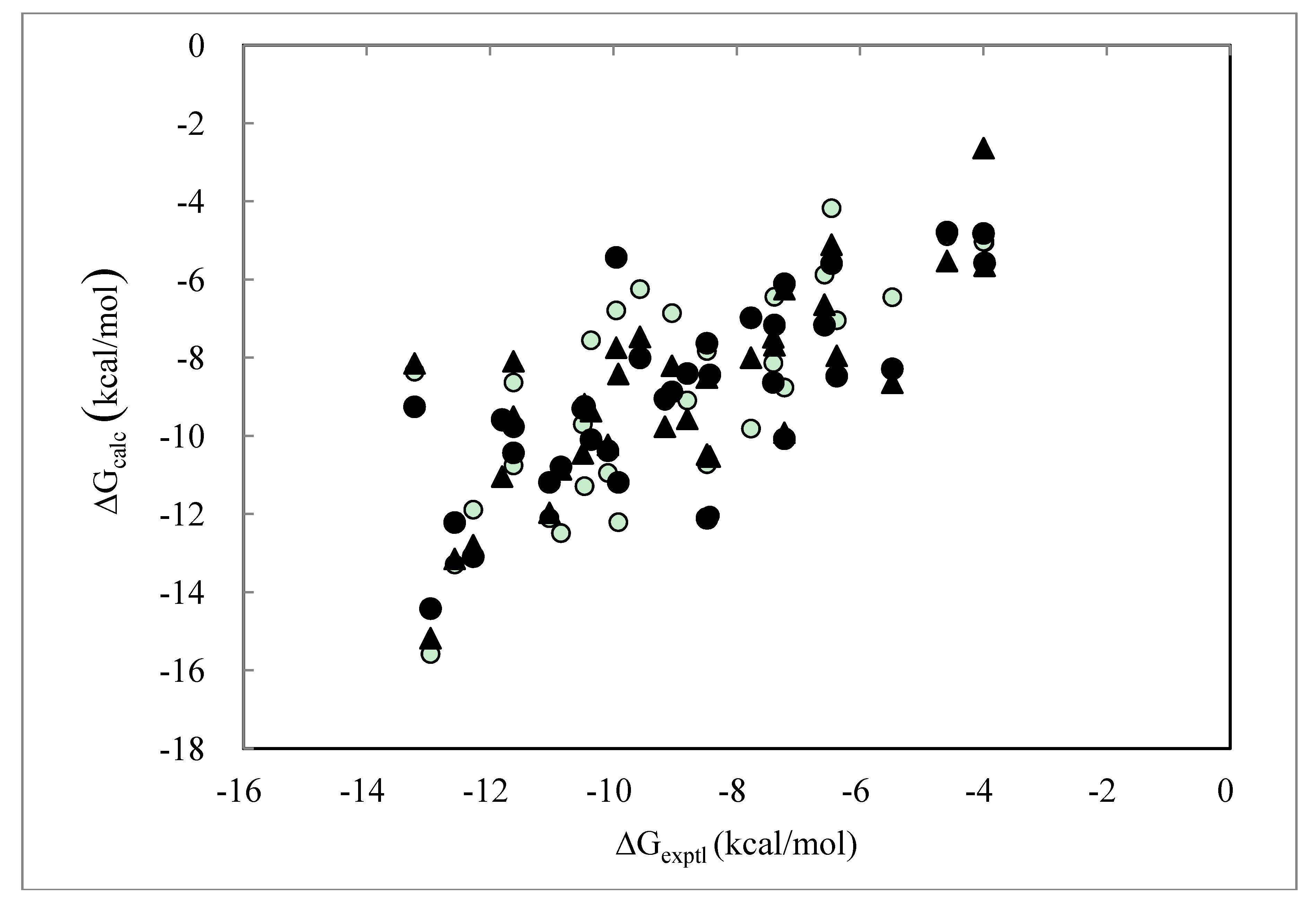
2.4. ΔG Estimation by the DIA Method


 > as in Equation (9).
| PDB ID | ΔGexptl | ΔGDIAV | ΔGDIAS | ΔGDIAV_L | ΔGDIAV_W | ΔGDIAV_LW | ΔGDIAV_LC |
|---|---|---|---|---|---|---|---|
| Equation (1) | Equation (3) | Equation (10) | Equation (11) | Equation (12) | Equation (9,12) | ||
| 1abf | −7.39 | −6.44 | −7.46 | −7.33 | −6.35 | −7.16 | −7.68 |
| 1apu | −10.50 | −9.70 | −10.70 | −9.00 | −9.70 | −9.30 | −10.45 |
| 1dbb | −12.27 | −11.89 | −11.25 | −12.08 | −11.67 | −13.09 | −12.80 |
| 1dbj | −10.47 | −11.28 | −10.39 | −11.35 | −11.07 | −9.24 | −9.19 |
| 1dog | −5.48 | −6.45 | −8.58 | −8.00 | −6.38 | −8.28 | −8.64 |
| 1dwb | −3.98 | −5.04 | −5.16 | −5.24 | −4.92 | −5.57 | −5.65 |
| 1epo | −10.85 | −12.49 | −12.35 | −13.13 | −12.53 | −10.79 | −10.85 |
| 1etr | −10.09 | −10.95 | −9.86 | −9.90 | −10.87 | −10.38 | −10.23 |
| 1ets | −11.62 | −10.75 | −10.21 | −10.48 | −10.62 | −10.43 | −9.51 |
| 1ett | −8.44 | −12.04 | −10.87 | −10.42 | −11.76 | −8.44 | −10.53 |
| 1hpv | −12.57 | −13.29 | −13.32 | −12.78 | −13.33 | −12.22 | −13.15 |
| 1hsl | −9.96 | −6.79 | −7.86 | −7.26 | −6.74 | −5.43 | −7.74 |
| 1htf | −11.04 | −12.10 | −10.45 | −11.48 | −12.13 | −11.19 | −11.97 |
| 1hvr | −12.97 | −15.58 | −14.97 | −15.33 | −15.63 | −14.42 | −15.18 |
| 1nsd | −7.23 | −8.76 | −9.21 | −9.19 | −8.65 | −10.07 | −9.92 |
| 1pgp | −7.77 | −9.81 | −9.10 | −8.99 | −9.56 | −6.98 | −8.00 |
| 1phg | −11.81 | −9.63 | −9.57 | −10.59 | −9.53 | −9.58 | −11.04 |
| 1ppc | −8.80 | −9.09 | −8.55 | −9.44 | −9.10 | −8.40 | −9.56 |
| 1pph | −8.49 | −7.83 | −7.46 | −8.13 | −7.81 | −7.63 | −8.51 |
| 1rbp | −9.17 | −9.10 | −9.62 | −9.74 | −9.11 | −9.04 | −9.76 |
| 1tng | −4.00 | −5.03 | −5.39 | −5.48 | −4.98 | −4.82 | −2.64 |
| 1tnh | −4.59 | −4.89 | −5.53 | −5.26 | −4.83 | −4.78 | −5.52 |
| 1ulb | −7.23 | −6.18 | −5.90 | −6.06 | −5.99 | −6.10 | −6.25 |
| 2cgr | −9.92 | −12.21 | −11.20 | −11.16 | −11.99 | −11.19 | −8.41 |
| 2gbp | −10.36 | −7.55 | −9.23 | −8.63 | −7.45 | −10.09 | −9.37 |
| 2ifb | −7.41 | −8.13 | −7.89 | −7.08 | −8.15 | −8.63 | −7.48 |
| 2phh | −6.38 | −7.04 | −7.57 | −7.31 | −6.83 | −8.47 | −7.95 |
| 2r04 | −8.48 | −10.72 | −10.58 | −10.29 | −10.71 | −12.11 | −10.48 |
| 2tsc | −11.62 | −8.63 | −9.97 | −8.90 | −8.75 | −9.76 | −8.09 |
| 2ypi | −6.58 | −5.87 | −6.53 | −6.20 | −5.76 | −7.16 | −6.64 |
| 3ptb | −6.46 | −4.17 | −4.75 | −4.75 | −4.12 | −5.59 | −5.11 |
| 4dfr | −13.23 | −8.35 | −7.96 | −8.16 | −8.36 | −9.25 | −8.14 |
| 5abp | −9.05 | −6.86 | −8.12 | −7.46 | −6.77 | −8.87 | −8.21 |
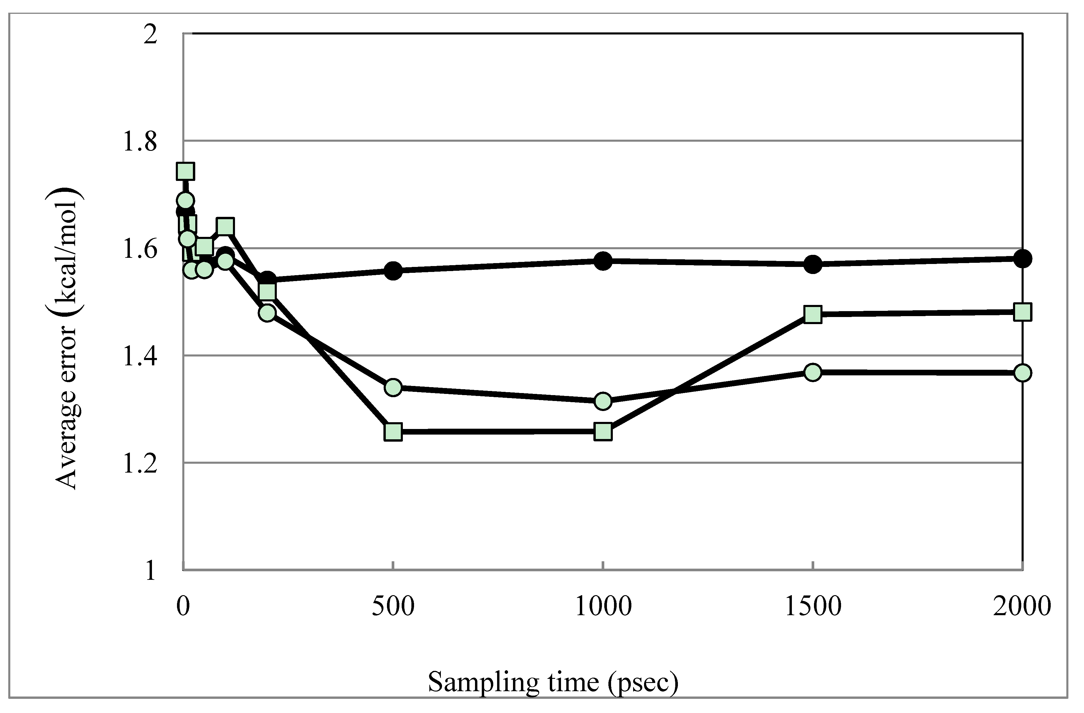
| Average Error | 1.58 | 1.36 | 1.39 | 1.48 | 1.26 | 1.31 | |
| SD a | 1.88 | 1.66 | 1.68 | 1.86 | 1.70 | 1.72 | |
| Correlation coefficient | 0.59 | 0.75 | 0.76 | 0.76 | 0.75 | 0.75 | |
| Average Error (MLR) b | 1.42 | 1.23 | 1.23 | 1.32 | 1.13 | 1.17 | |

| DIAV | α | β | τ | w |
| Average | 0.0341719 | 0.0017533 | −0.0002198 | 0.0000000 |
| Deviation (σ) | 0.0005495 | 0.0011874 | 0.0000087 | 0.0000000 |
| Min | 0.0323511 | −0.0038807 | −0.0002438 | 0.0000000 |
| Max | 0.0357564 | 0.0049798 | −0.0002027 | 0.0000000 |
| Negative value | 0.0000000 | 0.0285714 | 1.0000000 | 0.0000000 |
| DIAV_L | α | β | τ | w |
| Average | 0.0370196 | 0.0029651 | −0.0000050 | 0.1749169 |
| Deviation (σ) | 0.0007599 | 0.0008450 | 0.0000002 | 0.0190521 |
| Min | 0.0350933 | −0.0000641 | −0.0000054 | 0.1132383 |
| Max | 0.0396249 | 0.0047204 | −0.0000045 | 0.2325974 |
| Negative value | 0.0000000 | 0.0285714 | 1.0000000 | 0.0000000 |
| DIAV_W | α | β | τ | w |
| Average | 0.0346823 | 0.0021929 | −0.0002054 | 0.0000000 |
| Deviation (σ) | 0.0005388 | 0.0011036 | 0.0000083 | 0.0000000 |
| Min | 0.0329273 | −0.0030242 | −0.0002290 | 0.0000000 |
| Max | 0.0362899 | 0.0050095 | −0.0001878 | 0.0000000 |
| Negative value | 0.0000000 | 0.0285714 | 1.0000000 | 0.0000000 |
| DIAV_LW | α | β | τ | w |
| Average | 0.0413163 | 0.0062033 | −0. 0000067 | 0.1536118 |
| Deviation (σ) | 0.0007382 | 0.0007907 | 0. 0000002 | 0.0140040 |
| Min | 0.0392677 | 0.0034216 | −0. 0000071 | 0.1254044 |
| Max | 0.0434480 | 0.0087162 | −0. 0000063 | 0.1944447 |
| Negative value | 0.0000000 | 0.0000000 | 1.0000000 | 0.0000000 |
| DIAV_LC | α | β | τ | w |
| Average | 0.0343046 | 0.0042958 | −0.0000070 | 0.1143295 |
| Deviation (σ) | 0.0006129 | 0.0011950 | 0.0000002 | 0.0097216 |
| Min | 0.0321378 | 0.0002835 | −0.0000076 | 0.0942835 |
| Max | 0.0363001 | 0.0090566 | −0.0000067 | 0.1414504 |
| Negative value | 0.0000000 | 0. 0000000 | 1.0000000 | 0.0000000 |
| DIAS | α | β | τ | w |
| Average | 0.0392333 | 0.0030804 | −0.0000053 | 0.0000000 |
| Deviation (σ) | 0.0005573 | 0.0010426 | 0.0000002 | 0.0000000 |
| Min | 0.0375654 | −0.0017236 | −0.0000056 | 0.0000000 |
| Max | 0.0409116 | 0.0055269 | −0.0000049 | 0.0000000 |
| Negative value | 0.0000000 | 0.0285714 | 1.0000000 | 0.0000000 |

| PDB ID | ΔGexptl | ΔGDIAV_L | ||||||
|---|---|---|---|---|---|---|---|---|
| Original ligand | Alprenolol | Difference a | Fenoterol | Difference a | Cetirizine | Difference a | ||
| 1abe2 | −9.57 | −8.06 | −6.85 | −1.22 | −8.21 | 0.14 | −9.28 | 1.22 |
| 1abf1 | −7.39 | −8.40 | −6.13 | −2.27 | −6.72 | −1.68 | −7.93 | −0.47 |
| 1apu | −10.50 | −11.63 | −2.77 | −8.86 | −4.50 | −7.12 | −5.69 | −5.93 |
| 1cbx | −8.65 | −8.89 | −5.84 | −3.04 | −7.51 | −1.38 | −8.30 | −0.58 |
| 1dog | −5.48 | −9.05 | −5.18 | −3.87 | −7.75 | −1.30 | −5.08 | −3.97 |
| 1dwb | −3.98 | −5.45 | −5.44 | −0.01 | −6.56 | 1.11 | −8.24 | 2.80 |
| 1ebg | −14.76 | −6.74 | 0.00 | −6.74 | 0.00 | −6.74 | 0.00 | −6.74 |
| 1epo | −10.85 | −14.42 | −5.64 | −8.78 | −7.30 | −7.12 | −8.49 | −5.93 |
| 1rbp | −9.17 | −8.76 | N.D.b | N.D. b | N.D. b | N.D. b | −8.69 | −0.08 |
| 1stp | −18.27 | −6.59 | N.D. b | N.D. b | N.D. b | N.D. b | −5.96 | −0.63 |
| 1tnh | −4.59 | −5.59 | −4.39 | −1.20 | −5.62 | 0.03 | −6.13 | 0.54 |
| 1ulb | −7.23 | −6.19 | −5.45 | −0.74 | −6.23 | 0.04 | −8.98 | 2.79 |
| 2gbp | −10.36 | −10.14 | −7.16 | −2.98 | −8.74 | −1.40 | −10.24 | 0.11 |
| 2ifb | −7.41 | −8.60 | −5.81 | −2.79 | −7.09 | −1.51 | −9.01 | 0.41 |
| 2tsc | −11.62 | −8.23 | −5.68 | −2.55 | −6.48 | −1.75 | −8.69 | 0.47 |
| 2ypi | −6.58 | −6.92 | −4.68 | −2.24 | N.D. b | N.D. b | N.D. b | N.D. b |
| 3ptb | −6.46 | −4.96 | −4.49 | −0.48 | −5.89 | 0.93 | −5.64 | 0.68 |
| 4dfr | −13.22 | −8.42 | −5.16 | −3.26 | −5.64 | −2.79 | −6.66 | −1.76 |
| 6cpa | −15.71 | −11.68 | −6.82 | −4.86 | −7.77 | −3.91 | −9.75 | −1.93 |
| Average | −9.57 | −8.35 | −5.15 | −3.29 | −6.38 | −2.15 | −7.38 | −1.06 |
| Thrombin | ΔGexptl | ΔGDIAV_L | Error | ΔGDIAV_LW | Error | ΔGDIAV_LC | Error |
|---|---|---|---|---|---|---|---|
| 1dwb | −3.98 | −5.15 | 1.17 | −5.02 | 1.04 | −5.57 | 1.59 |
| 1ett | −8.44 | −9.9 | 1.46 | −9.74 | 1.31 | −9.81 | 1.37 |
| 1etr | −10.09 | −9.9 | 0.19 | −9.89 | 0.2 | −10.22 | 0.13 |
| 1ets | −11.62 | −10.9 | 0.72 | −10.76 | 0.86 | −10.46 | 1.16 |
| Averaged error (kcal/mol) | - | - | 0.89 | - | 0.85 | - | 1.06 |
| SDa | - | - | 1.01 | - | 0.95 | - | 1.20 |
| Correlation coefficient | - | - | 0.97 | - | 0.97 | - | 0.96 |
| Spearman’s rank correlation | - | - | 1 | - | 1 | - | 1 |
| HIV-1 Protease | ΔGexptl | ΔGDIAV_L | Error | ΔGDIAV_LW | Error | ΔGDIAV_LC | Error |
| 1k6p | −8.84 | −11.71 | 2.87 | −11.74 | 2.90 | −11.78 | 2.94 |
| 1ajv | −10.59 | −10.36 | 0.23 | −10.39 | 0.20 | −10.13 | 0.46 |
| 1ajx | −10.86 | −9.89 | 0.97 | −9.91 | 0.95 | −9.68 | 1.18 |
| 1hih | −10.97 | −11.67 | 0.70 | −11.67 | 0.70 | −11.73 | 0.76 |
| 1htf | −11.04 | −11.57 | 0.53 | −11.59 | 0.55 | −11.86 | 0.82 |
| 1aaq | −11.45 | −13.15 | 1.70 | −13.13 | 1.68 | −12.96 | 1.51 |
| 1hpv | −12.57 | −12.79 | 0.22 | −12.87 | 0.30 | −13.06 | 0.49 |
| 1hvr | −12.97 | −14.79 | 1.82 | −14.93 | 1.96 | −14.65 | 1.68 |
| 1hvk | −13.79 | −13.63 | 0.16 | −13.65 | 0.14 | −13.70 | 0.09 |
| 1vj | −14.62 | −12.82 | 1.80 | −12.85 | 1.77 | −12.89 | 1.73 |
| 1dif | −14.63 | −13.76 | 0.87 | −13.77 | 0.86 | −13.82 | 0.81 |
| Averaged error (kcal/mol) | - | - | 1.08 | - | 1.09 | - | 1.13 |
| SDa | - | - | 1.36 | - | 1.37 | - | 1.37 |
| Correlation coefficient | - | - | 0.68 | - | 0.67 | - | 0.68 |
| Spearman’s rank correlation | - | - | 0.78 | - | 0.75 | - | 0.81 |
| Trypsin | ΔGexptl | ΔGDIAV_L | Error | ΔGDIAV_LW | Error | ΔGDIAV_LC | Error |
| 1tng | −4.00 | −5.45 | 1.45 | −5.36 | 1.37 | −2.69 | 1.31 |
| 1tnh | −4.59 | −5.29 | 0.70 | −5.20 | 0.61 | −5.50 | 0.91 |
| 3ptb | −6.46 | −4.92 | 1.54 | −4.83 | 1.63 | −5.15 | 1.31 |
| 1pph | −8.48 | −8.32 | 0.16 | −8.30 | 0.18 | −8.51 | 0.02 |
| 1ppc | −8.80 | −9.32 | 0.52 | −9.31 | 0.51 | −9.53 | 0.72 |
| Averaged error (kcal/mol) | - | - | 0.88 | - | 0.86 | - | 0.86 |
| SDa | - | - | 1.03 | - | 1.02 | - | 0.98 |
| Correlation coefficient | - | - | 0.86 | - | 0.86 | - | 0.93 |
| Spearman’s rank correlation | - | - | 0.60 | - | 0.60 | - | 0.90 |
2.5. Consensus Score with the Trajectory Average of the Docking Score
3. Method: The Docking Score Calculation

4. Data Preparation
| PDB ID | Protein | Ligand | MW | HA | HD |
|---|---|---|---|---|---|
| 1abe | l-arabinose-binding protein | l-arabinose | 150.1 | 5 | 4 |
| 1abf | l-arabinose-binding protein | d-fucose | 161.2 | 5 | 4 |
| 1apu | acid proteinase (penicillopepsin) | pepstatin | 485.7 | 6 | 4 |
| 1dbb | Fab' fragment | progesterone | 314.5 | 2 | 0 |
| 1dbj | Fab' fragment | aetiocholanolone | 290.4 | 2 | 1 |
| 1dog | glucoamylase | deoxynojirimycin | 163.2 | 4 | 5 |
| 1dwb | thrombin | benzamidine | 120.2 | 0 | 2 |
| 1epo | endothia aspartic proteinase | n-carbonylmorpholine | 131.1 | 5 | 6 |
| 1etr | thrombin | MQPA | 509.2 | 5 | 5 |
| 1ets | thrombin | NAPAP | 522.6 | 4 | 4 |
| 1ett | thrombin | 4-tapap | 429.6 | 3 | 3 |
| 1hpv | HIV-1 protease | amprenavir | 505.6 | 6 | 3 |
| 1hsl | Histidine-binding protein | Histidine | 156.2 | 3 | 2 |
| 1htf | HIV-1 protease | GR126045 | 574.7 | 4 | 5 |
| 1hvr | HIV-1 protease | XK263 | 606.8 | 3 | 2 |
| 1nsd | neuraminidase | neuraminic acid | 290.2 | 8 | 5 |
| 1pgp | 6-phosphogluconate dehydrogenase | 6-phosphogluconic acid | 276.1 | 10 | 4 |
| 1phg | cytochrome P450 | metyrapone | 226.3 | 3 | 0 |
| 1ppc | trypsin | Napap | 533.6 | 4 | 4 |
| 1pph | trypsin | 3-Tapap | 429.6 | 3 | 3 |
| 1rbp | retinol-binding protein | retinol | 286.5 | 1 | 1 |
| 1tng | trypsin | aminomethylcyclohexane | 114.2 | 0 | 1 |
| 1tnh | trypsin | 4-fluorobenzylamine | 126.2 | 0 | 1 |
| 1ulb | purine nucleoside phosphorylase | guanine | 151.1 | 3 | 3 |
| 2cgr | Igg2b (KAPPA) Fab fragment | guanidineacetic acid | 384.4 | 3 | 3 |
| 2gbp | d-galactose / D-glucose-binding protein | d-glucose | 180.2 | 6 | 5 |
| 2ifb | intestinal fatty acid binding protein | palmitic acid | 256.4 | 2 | 0 |
| 2phh | p-hydroxybenzoate hydroxylase | p-hydroxybenzoate | 138.1 | 3 | 1 |
| 2r04 | rhinovirus 14 (HRV14) | W71 | 342.4 | 5 | 0 |
| 2tsc | thymidylate synthase | 10-propargyl-5,8-dideazafolic acid | 477.5 | 7 | 3 |
| 2ypi | triose phosphate isomerase | 2-phosphoglycolate | 156.0 | 6 | 0 |
| 3ptb | trypsin | benzamidine | 120.2 | 0 | 2 |
| 4dfr | dihydrofolate reductase | methotrexate | 454.4 | 9 | 3 |
| 5abp | l-arabinose-binding protein | d-galactose | 180.2 | 6 | 5 |
5. Conclusions
Acknowledgements
References
- Warren, G.L.; Andrews, C.W.; Capelli, A.M.; Clarke, B.; LaLonde, J.; Lambert, M.H.; Lindvall, M.; Nevins, N.; Semus, S.F.; Senger, S.; et al. A critical assessment of docking programs and scoring functions. J. Med. Chem. 2006, 49, 5912–5931. [Google Scholar] [CrossRef]
- Kontoyianni, M.; Sokol, G.S.; McClellan, L.M. Evaluation of library ranking efficacy in virtual screening. J. Comput. Chem. 2005, 26, 11–22. [Google Scholar] [CrossRef]
- Kuntz, I.D.; Blaney, J.M.; Oatley, S.J.; Langridge, R.; Ferrin, T.E. A geometric approach to macromolecule-ligand interactions. J. Mol. Biol. 1982, 161, 269–288. [Google Scholar] [CrossRef]
- Rarey, M.; Kramer, B.; Lengauer, T.; Klebe, G. A fast flexible docking method using an incremental construction algorithm. J. Mol. Biol. 1996, 261, 470–489. [Google Scholar] [CrossRef]
- Jones, G.; Willet, P.; Glen, R.C.; Leach, A.R.; Taylor, R. Development and validation of a genetic algorithm for flexible docking. J. Mol. Biol. 1997, 267, 727–748. [Google Scholar] [CrossRef]
- Baxter, C.A.; Murray, C.W.; Clark, D.E.; Westhead, D.R.; Eldridge, M.D. Flexible docking using tabu search and an empirical estimate of binding affinity. Proteins 1998, 33, 367–382. [Google Scholar] [CrossRef]
- Fukunishi, Y.; Mikami, Y.; Nakamura, H. Similarities among receptor pockets and among compounds: Analysis and application to in silico ligand screening. J. Mol. Graph. Model. 2005, 24, 34–45. [Google Scholar] [CrossRef]
- Zhang, C.; Liu, S.; Zhu, Q.; Zhou, Y. A knowledge-based energy function for protein-ligand, protein–protein, and protein-DNA complexes. J. Med. Chem. 2005, 48, 2325–2335. [Google Scholar] [CrossRef]
- Muegge, I.; Martin, Y.C. A general and fast scoring function for protein-ligand interactions: A simplified potential approach. J. Med. Chem. 1999, 42, 791–804. [Google Scholar] [CrossRef]
- Fukunishi, Y.; Mikami, Y.; Kubota, S.; Nakamura, H. Multiple target screening method for robust and accurate in silico ligand screening. J. Mol. Graphics Modell. 2005, 25, 61–70. [Google Scholar]
- Shan, Y.; Kim, T.E.; Eastwood, M.P.; Dror, R.O.; Seeliger, M.A.; Shaw, D.E. How does a drug molecule find its target binding site? J. Am. Chem. Soc. 2011, 133, 9181–9183. [Google Scholar]
- Dror, R.O.; Pan, A.C.; Arlow, D.H.; Borhani, D.W.; Maragakis, P.; Shan, Y.; Xu, H.; Shaw, D.E. Pathway and mechanism of drug binding to G-protein-coupled receptors. Proc. Natl. Acad. Soc. USA 2011, 108, 13118–13123. [Google Scholar] [CrossRef]
- Kamiya, N.; Yonezawa, Y.; Nakamura, H.; Higo, J. Protein-inhibitor flexible docking by a multicanonical sampling: Native complex structure with the lowest free energy and a free-energy barrier distinguishing the native complex from the others. Proteins 2008, 70, 41–53. [Google Scholar]
- Nakajima, N.; Higo, J.; Kidera, A.; Nakamura, H. Flexible docking of a ligand peptide to a receptor protein by multicanonical molecular dynamics simulation. Chem. Phys. Lett. 1997, 278, 297–301. [Google Scholar] [CrossRef]
- Fukunishi, Y.; Mikami, Y.; Nakamura, H. The filling potential method: A method for estimating the free energy surface for protein-ligand docking. J. Phys. Chem. B 2003, 107, 13201–13210. [Google Scholar] [CrossRef]
- Gervasio, F.L.; Laio, A.; Parrinello, M. Flexible docking in solution using metadynamics. J. Am. Chem. Soc. 2005, 127, 2600–2607. [Google Scholar] [CrossRef]
- Branduardi, D.; Gervasio, F.L.; Parrinello, M. From A to B in free energy space. J. Chem. Phys. 2007, 126, 054103. [Google Scholar] [CrossRef]
- Fujitani, H.; Tanida, Y.; Matsuura, A. Massively parallel computation of absolute binding free energy with well-equilibrated states. Phys. Rev. E 2009, 79, 021914. [Google Scholar] [CrossRef]
- Fukunishi, Y.; Mitomo, D.; Nakamura, H. Protein-ligand binding free energy calculation by the smooth reaction path generation SRPG method. J. Chem. Inf. Model. 2009, 49, 1944–1951. [Google Scholar] [CrossRef]
- Liphardt, J.; Dumont, S.; Smith, S.B.; Tinoco, I., Jr.; Bustamante, C. Equilibrium information from nonequilibrium measurements in an experimental test of Jarzynski’s equality. Science 2002, 296, 1832–1835. [Google Scholar] [CrossRef]
- Kollman, P.A.; Massova, I.; Reyes, C.; Kuhn, B.; Huo, S.; Chong, L.; Lee, M.; Lee, T.; Duan, Y.; Wang, W.; et al. Calculating structures and free energies of complex molecules: Combining molecular mechanics and continuum models. Acc. Chem. Res. 2000, 33, 889–897. [Google Scholar] [CrossRef]
- Hansson, T.; Marelius, J.; Åqvist, J. Ligand binding affinity prediction by linear interaction energy methods. J. Comput. Aided. Mol. Des. 1998, 12, 27–35. [Google Scholar] [CrossRef]
- Pisabarro, T.M.; Gago, F.; Wade, R.C. Prediction of drug binding affinities by comparative binding energy analysis. J. Med. Chem. 1995, 38, 2681–2691. [Google Scholar] [CrossRef]
- Cuevas, C.; Pastor, M.; Perez, C.; Gago, F. Comparative binding energy (COMBINE) analysis of human neutrophil elastase inhibition by pyridone-containing trifluoromethylketones. Comb. Chem. High. Throughput Screen 2001, 4, 627–642. [Google Scholar] [CrossRef]
- Pastor, M.; Ortiz, A.R.; Gago, F. Comparative binding energy analysis of HIV-1 protease inhibitors: incorporation of solvent effects and validation as a powerful tool in receptor-based drug design. J. Med. Chem. 1998, 41, 836–852. [Google Scholar] [CrossRef]
- Lozano, J.J.; Pastor, M.; Cruciani, G.; Gaedt, K.; Centeno, N.B.; Gago, F.; Sanz, F. 3D-QSAR methods on the basis of ligand-receptor complexes. Application of COMBINE and GRID/GOLPE methodologies to a series of CYP1A2 ligands. J. Comput. Aided Mol. Des. 2000, 14, 341–353. [Google Scholar] [CrossRef]
- Tomic, S.; Nilsson, L.; Wade, R.C. Nuclear receptor—DNA binding specificity: A COMBINE and Free-Wilson QSAR analysis. J. Med. Chem. 2000, 43, 1780–1792. [Google Scholar] [CrossRef]
- Wang, T.; Wade, R.C. Comparative binding energy (COMBINE) analysis of influenza neuraminidase-inhibitor complexes. J. Med. Chem. 2001, 44, 961–971. [Google Scholar] [CrossRef]
- Murcia, M.; Ortiz, A.R. Virtual screening with flexible docking and COMBINE-based models. Application to a series of factor Xa inhibitors. J. Med. Chem. 2004, 47, 805–820. [Google Scholar] [CrossRef]
- Fukunishi, Y.; Nakamura, H. Statistical estimation of the protein-ligand binding free energy based on direct protein-ligand interaction obtained by molecular dynamics simulation. Pharmaceuticals 2012, 5, 1064–1079. [Google Scholar] [CrossRef]
- Abel, R.; Young, T.; Farid, R.; Beme, B.J.; Friesner, R.A. Role of the active-site solvent in the thermodynamics of factor Xa ligand binding. J. Am. Chem. Soc. 2008, 130, 2817–2831. [Google Scholar] [CrossRef]
- Repasky, M.P.; Murphy, R.B.; Banks, J.L.; Greenwood, J.R.; Tubert-brohman, I.; Bhat, S.; Friesner, R.A. Docking performance of the glide program as evaluated on the Astex and DUD database: A complete set of glide SP results and selected results for a new scoring function integrating WaterMap and glide. J. Comput. Aided Mol. Des. 2012, 26, 787–799. [Google Scholar] [CrossRef]
- Case, D.A.; Darden, T.A.; Cheatham, T.E., III; Simmerling, C.L.; Wang, J.; Duke, R.E.; Luo, R.; Merz, K.M.; Wang, B.; Pearlman, D.A.; et al. AMBER 8, University of California: San Francisco, CA, USA, 2004.
- Wang, J.; Wolf, R.M.; Caldwell, J.W.; Kollman, P.A.; Case, D.A. Development and testing of a general amber force field. J. Compt. Chem. 2004, 25, 1157–1174. [Google Scholar] [CrossRef]
- Bairgya, H.R.; Mukhopadhyay, B.P.; Bhattacharya, S. Role of the conserved water molecules in the binding of inhibitor to IMPDH-II (human): A study on the water mimic inhibitor design. J. Mol. Struct. 2009, 908, 31–39. [Google Scholar] [CrossRef]
- Mobley, D.L. Let’s get honest about sampling. J. Comput. Aided Mol. Des. 2012, 26, 93–95. [Google Scholar] [CrossRef]
- Ballester, P.J.; Mitchell, J.B.O. A machine learning approach to predicting protein-ligand binding affinity with applications to molecular docking. Bioinformatics 2010, 26, 1169–1175. [Google Scholar] [CrossRef]
- Kawabata, T. Build-up algorithm for atomic correspondence between chemical structures. J. Chem. Inf. Mod. 2011, 51, 1775–1787. [Google Scholar] [CrossRef]
- Wang, J.; Cieplak, P.; Kollman, P.A. How well does a restrained electrostatic potential (RESP) model perform in calculating conformational energies of organic and biological molecules? J. Comput. Chem. 2000, 21, 1049–1074. [Google Scholar] [CrossRef]
- Frisch, M.J.; Trucks, G.W.; Schlegel, H.B.; Scuseria, G.E.; Robb, M.A.; Cheeseman, J.R.; Zakrzewski, V.G.; Montgomery, J.A.; Stratmann, R.E., Jr.; Burant, J.C.; et al. Gaussian 98, Revision A.9, Gaussian, Inc.: Pittsburgh, PA, USA, 1998.
- Jorgensen, W.L.; Chandrasekhar, J.; Madura, J.D.; Impey, R.W.; Klein, M.L. Comparison of simple potential functions for simulating lipid water. J. Chem. Phys. 1983, 79, 926–935. [Google Scholar] [CrossRef]
- Ryckaert, J.P.; Ciccotti, G.; Berendsen, H.J.C. Numerical integration of the cartesian equations of motion of a system with constraints: Molecular dynamics of n-alkanes. J. Comput. Phys. 1977, 23, 327–341. [Google Scholar] [CrossRef]
- Greengard, L.; Rokhlin, V. A fast algorithm for particle simulations. J. Comput. Phys. 1987, 73, 325–348. [Google Scholar] [CrossRef]
Supplementary Files
© 2013 by the authors; licensee MDPI, Basel, Switzerland. This article is an open access article distributed under the terms and conditions of the Creative Commons Attribution license (http://creativecommons.org/licenses/by/3.0/).
Share and Cite
Fukunishi, Y.; Nakamura, H. Improved Estimation of Protein-Ligand Binding Free Energy by Using the Ligand-Entropy and Mobility of Water Molecules. Pharmaceuticals 2013, 6, 604-622. https://doi.org/10.3390/ph6050604
Fukunishi Y, Nakamura H. Improved Estimation of Protein-Ligand Binding Free Energy by Using the Ligand-Entropy and Mobility of Water Molecules. Pharmaceuticals. 2013; 6(5):604-622. https://doi.org/10.3390/ph6050604
Chicago/Turabian StyleFukunishi, Yoshifumi, and Haruki Nakamura. 2013. "Improved Estimation of Protein-Ligand Binding Free Energy by Using the Ligand-Entropy and Mobility of Water Molecules" Pharmaceuticals 6, no. 5: 604-622. https://doi.org/10.3390/ph6050604