NO2 and Cancer Incidence in Saudi Arabia

Abstract
:1. Introduction
2. Materials and Methods
2.1. Cancer Data
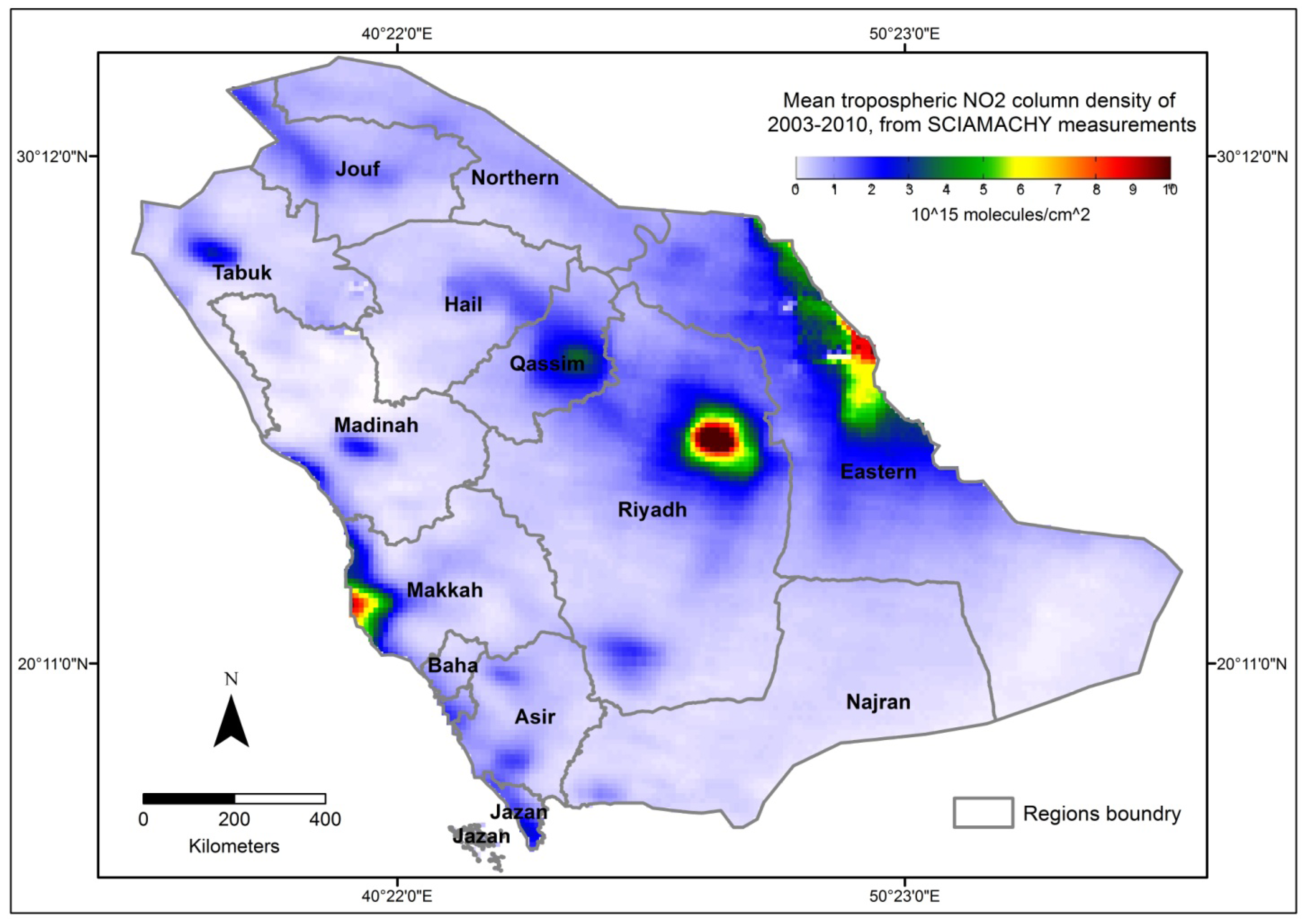
2.2. NO2 Data

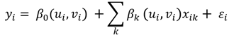
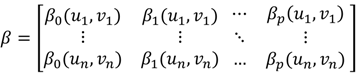
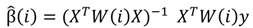
2.3. Spatial Statistical Analysis


 is the estimate of the standard deviation of the residuals, and tr(S) is the trace of the hat matrix. The AIC can be used to compare models of the same independent variable and compare the global OLS model with a local GWR model [57]. The OLS and GWR models were fitted and mapped using ESRI ArcGIS 10.1.
3. Results

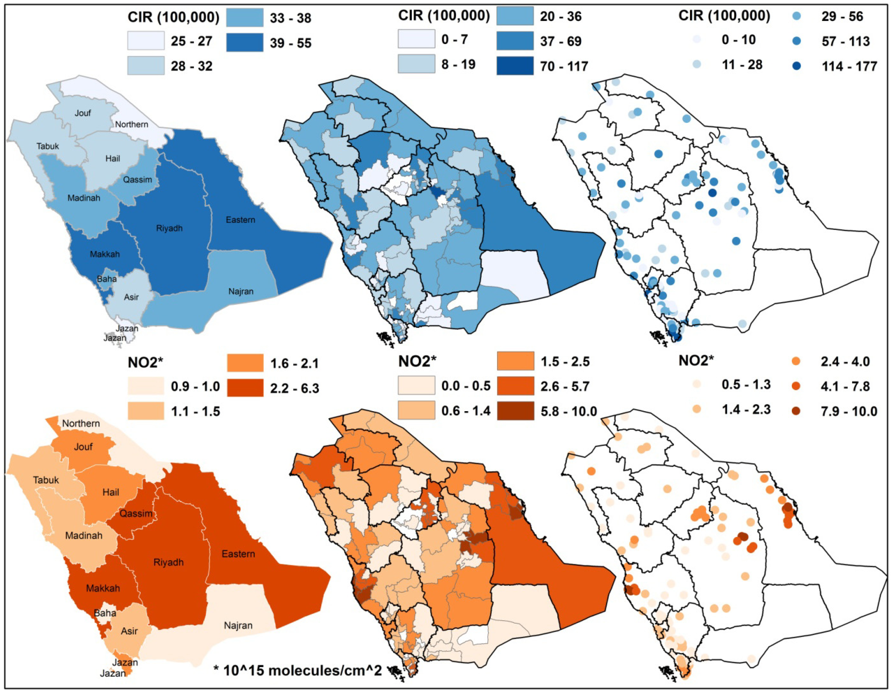
| Region | All Cases | Males | Females | Avg. NO2 | |||||||||
|---|---|---|---|---|---|---|---|---|---|---|---|---|---|
| Number | Percent | CIR | ASR | Number | Percent | CIR | ASR | Number | Percent | CIR | ASR | ||
| Riyadh | 13,063 | 28.69 | 54.88 | 47.34 | 6,512 | 28.4 | 53.60 | 46.09 | 6,551 | 28.98 | 56.22 | 45.37 | 3.34 |
| Eastern | 7,698 | 16.9 | 46.42 | 41.41 | 3,867 | 16.86 | 45.54 | 43.31 | 3,830 | 16.95 | 47.35 | 38.53 | 6.28 |
| Makkah | 10,479 | 23.01 | 44.51 | 33.10 | 5,228 | 22.8 | 44.35 | 31.78 | 5,251 | 23.23 | 44.67 | 32.00 | 3.23 |
| Madinah | 2,855 | 6.27 | 38.57 | 28.63 | 1,442 | 6.29 | 39.40 | 28.98 | 1,413 | 6.25 | 37.76 | 27.72 | 1.39 |
| Qassim | 1,992 | 4.37 | 37.45 | 26.30 | 1,030 | 4.49 | 38.86 | 27.15 | 962 | 4.26 | 36.06 | 24.94 | 3.18 |
| Baha | 779 | 1.71 | 34.94 | 18.88 | 374 | 1.63 | 35.95 | 19.56 | 405 | 1.79 | 34.05 | 18.25 | 1.00 |
| Najran | 760 | 1.67 | 34.19 | 24.79 | 419 | 1.83 | 37.93 | 28.56 | 341 | 1.51 | 30.49 | 20.98 | 0.90 |
| Hail | 948 | 2.08 | 32.05 | 18.68 | 481 | 2.1 | 33.42 | 18.99 | 467 | 2.07 | 30.74 | 18.02 | 1.70 |
| Asir | 2,957 | 6.49 | 31.09 | 20.40 | 1,522 | 6.64 | 32.89 | 20.76 | 1,435 | 6.35 | 29.38 | 19.53 | 1.24 |
| Tabuk | 1,160 | 2.55 | 30.84 | 27.41 | 612 | 2.67 | 31.63 | 30.42 | 548 | 2.42 | 30.00 | 24.93 | 1.48 |
| Jouf | 586 | 1.29 | 29.50 | 21.83 | 306 | 1.33 | 30.75 | 22.78 | 280 | 1.24 | 28.25 | 20.71 | 1.78 |
| Northern | 430 | 0.94 | 27.55 | 21.16 | 210 | 0.92 | 26.91 | 21.63 | 220 | 0.97 | 28.19 | 21.05 | 0.93 |
| Jazan | 1,613 | 3.54 | 25.03 | 16.77 | 805 | 3.51 | 25.60 | 16.51 | 808 | 3.57 | 24.49 | 16.65 | 2.13 |

| Cancer | OLS-NO | OLS-CIR |
|---|---|---|
| All Cancers | 0.13 | 0.43 * |
| Liver | 0.21 | 0.06 |
| Breast | 0.50 * | 0.71 * |
| Colorectal | 0.40 * | 0.37 * |
| NHL | 0.38 * | 0.17 |
| Leukemia | 0.40 * | 0.12 |
| Thyroid | 0.41 * | 0.11 |
| Lung | 0.62 * | 0.59 * |
| Other Skin | 0.32 * | 0.00 ° |
| Hodgkin’s Disease | 0.55 * | 0.17 ° |
| Bladder | 0.55 * | 0.22 *° |
| Cervical | 0.46 * | 0.41 * |
| Ovarian | 0.38 * | 0.37 * |
| Prostate | 0.56 * | 0.61 * |
| Cancer | OLS-NO | OLS-CIR | GWR-NO | GWR-CIR |
|---|---|---|---|---|
| All Cancers | 0.31 *° | 0.06 * | 0.33 ° | 0.14 |
| Liver | 0.26 ° | 0.05 * | 0.26 ° | 0.10 |
| Brest | 0.33 *° | 0.09 *° | 0.39 ° | 0.39 |
| Colorectal | 0.32 *° | 0.06 * | 0.34 ° | 0.14 |
| NHL | 0.30 *° | 0.03 * | 0.33 ° | 0.06 |
| Leukemia | 0.28 *° | 0.04 * | 0.28 ° | 0.06 ° |
| Thyroid | 0.27 ° | 0.05 *° | 0.27 ° | 0.18 |
| Lung | 0.32 * | 0.02 ° | 0.43 | 0.44 ° |
| Other Skin | 0.28 *° | 0.005 | 0.30 ° | 0.03 |
| Hodgkin’s Disease | 0.30 *° | 0.03 ° | 0.31 ° | 0.17 |
| Bladder | 0.31 * | 0.007 ° | 0.33 ° | 0.08 |
| Cervical | 0.33 * | 0.05 * | 0.42 ° | 0.15 |
| Ovarian | 0.33 * | 0.02 | 0.39 ° | 0.05 |
| Prostate | 0.31 *° | 0.05 ° | 0.33 ° | 0.31 |
| Cancer | OLS-NO | OLS-CIR | GWR-NO | GWR-CIR |
|---|---|---|---|---|
| All Cancers | 0.17 ° | 0.03 ° | 0.23 | 0.17 ° |
| Liver | 0.13 ° | 0.0002 | 0.17 | 0.22 ° |
| Brest | 0.20 *° | 0.10 *° | 0.29 | 0.11 ° |
| Colorectal | 0.17 ° | 0.05 *° | 0.24 | 0.06 ° |
| NHL | 0.16 ° | 0.006 ° | 0.24 | 0.14 ° |
| Leukemia | 0.14 ° | 0.006 ° | 0.18 | 0.14 ° |
| Thyroid | 0.14 ° | 0.017 ° | 0.17 | 0.08 ° |
| Lung | 0.23 * | 0.11 *° | 0.33 | 0.13 ° |
| Other Skin | 0.15 ° | 0.0003 | 0.20 | 0.21 ° |
| Hodgkin’s Disease | 0.17 | 0.005 ° | 0.22 | 0.22 |
| Bladder | 0.17 * | 0.008° | 0.25 | 0.19 ° |
| Cervical | 0.18 *° | 0.04 *° | 0.30 | 0.05 ° |
| Ovarian | 0.18 *° | 0.007 ° | 0.29 | 0.09 ° |
| Prostate | 0.18 *° | 0.10 *° | 0.24 | 0.14 ° |
4. Discussion
5. Conclusions
Acknowledgments
Conflicts of Interest
References
- WHO (World Health Organization), Regional Office for Europe Health, Health Aspects of Air Pollution with Particulate Matter, Ozone and Nitrogen Dioxide; WHO Regional Office for Europe: Bonn, Germany, 2003.
- Barillaro, G.; Diligenti, A.; Strambini, L.M.; Comini, E.; Faglia, G. NO2 adsorption effects on p+-n silicon junctions surrounded by a porous layer. Sensors Actuat. B Chem. 2008, 134, 922–927. [Google Scholar] [CrossRef]
- Beeson, W.L.; Abbey, D.E.; Knutsen, S.F. Long-term concentrations of ambient air pollutants and incident lung cancer in California adults: Results from the AHSMOG study. Adventist Health Study on Smog. Environ. Health Perspect. 1998, 106, 813–823. [Google Scholar] [CrossRef]
- Nyberg, F.; Gustavsson, P.; Järup, L.; Bellander, T.; Berglind, N.; Jakobsson, R.; Pershagen, G. Urban air pollution and lung cancer in Stockholm. Epidemiology 2000, 11, 487–495. [Google Scholar] [CrossRef]
- Nafstad, P.; Haheim, L.L.; Oftedal, B.; Gram, F.; Holme, I.; Hjermann, I.; Leren, P. Lung cancer and air pollution: A 27 year follow up of 16 209 Norwegian men. Thorax 2003, 58, 1071–1076. [Google Scholar] [CrossRef]
- Dockery, D.W.; Pope, C.A.; Xu, X.; Spengler, J.D.; Ware, J.H.; Fay, M.E.; Ferris, B.G., Jr.; Speizer, F.E. An association between air pollution and mortality in six US cities. N. Engl. J. Med. 1993, 329, 1753–1759. [Google Scholar] [CrossRef]
- Pope, C.A.; Thun, M.J.; Namboodiri, M.M.; Dockery, D.W.; Evans, J.S.; Speizer, F.E.; Heath, C.W. Particulate air pollution as a predictor of mortality in a prospective study of US adults. Am. J. Respir. Crit. Care Med. 1995, 151, 669–674. [Google Scholar] [CrossRef]
- Pope, C.A., III; Burnett, R.T.; Thun, M.J.; Calle, E.E.; Krewski, D.; Ito, K.; Thurston, G.D. Lung cancer, cardiopulmonary mortality, and long-term exposure to fine particulate air pollution. JAMA 2002, 287, 1132–1141. [Google Scholar] [CrossRef]
- Vineis, P.; Hoek, G.; Krzyzanowski, M.; Vigna-Taglianti, F.; Veglia, F.; Airoldi, L.; Autrup, H.; Dunning, A.; Garte, S.; Hainaut, P.; et al. Air pollution and risk of lung cancer in a prospective study in Europe. Int. J. Cancer 2006, 119, 169–174. [Google Scholar] [CrossRef]
- Vineis, P.; Hoek, G.; Krzyzanowski, M.; Vigna-Taglianti, F.; Veglia, F.; Airoldi, L.; Overvad, K.; Raaschoi-Nielsen, O.; Clavel-Chapelon, F.; Linseisen, J.; et al. Lung cancers attributable to environmental tobacco smoke and air pollution in non-smokers in different European countries: A prospective study. Environ. Health 2007, 6. [Google Scholar] [CrossRef] [Green Version]
- Katanoda, K.; Sobue, T.; Satoh, H.; Tajima, K.; Suzuki, T; Nakatsuka, H.; Takezaki, T.; Nakayama, T.; Nitta, H.; Tanabe, K.; et al. An association between long-term exposure to ambient air pollution and mortality from lung cancer and respiratory diseases in Japan. J. Epidemiol. 2011, 21, 132–143. [Google Scholar] [CrossRef]
- Raaschou-Nielsen, O.; Andersen, Z.J.; Hvidberg, M.; Jensen, S.S.; Ketzel, M.; Sørensen, M.; Loft, S.; Overvad, K.; Tjønneland, A. Lung cancer incidence and long-term exposure to air pollution from traffic. Environ. Health Perspect. 2011, 119, 860–865. [Google Scholar] [CrossRef]
- Castaño-Vinyals, G.; Cantor, K.P.; Malats, N.; Tardon, A.; Garcia-Closas, R.; Serra, C.; Carrato, A.; Rothman, N.; Vermeulen, R.; Silverman, D.; et al. Air pollution and risk of urinary bladder cancer in a case-control study in Spain. Occup. Environ. Med. 2008, 65, 56–60. [Google Scholar] [CrossRef]
- Liu, C.C.; Tsai, S.S.; Chiu, H.F.; Wu, T.N.; Chen, C.C.; Yang, C.Y. Ambient exposure to criteria air pollutants and risk of death from bladder cancer in Taiwan. Inhal. Toxicol. 2010, 21, 48–54. [Google Scholar]
- Crouse, D.L.; Goldberg, M.S.; Ross, N.A.; Chen, H.; Labreche, F. Postmenopausal breast cancer is associated with exposure to traffic-related air pollution in Montreal, Canada: A case-control study. Environ. Health Perspect. 2010, 118, 1578–1583. [Google Scholar] [CrossRef]
- Raaschou-Nielsen, O.; Andersen, Z.J.; Hvidberg, M.; Jensen, S.S.; Ketzel, M.; Sørensen, M.; Hansen, J.; Loft, S.; Overvad, K.; Tjønneland, A. Air pollution from traffic and cancer incidence: A Danish cohort study. Environ. Health 2011, 10, 67. [Google Scholar] [CrossRef]
- Rosenlund, M.; Bellander, T.; Nordquist, T.; Alfredsson, L. Long-term exposure to air pollution and cancer. Epidemiology 2007, 18, S66. [Google Scholar]
- Kan, H.; Gu, D. Association between Long-Term Exposure to Outdoor Air Pollution and Mortality in China: A Cohort Study. In Proceedings of the ISEE 22nd Annual Conference, Seoul, Korea, 28 August–1 September 2010.
- Yorifuji, T.; Kashima, S.; Tsuda, T.; Ishikawa-Takata, K.; Ohta, T.; Tsuruta, K.; Doi, H. Long-term exposure to traffic-related air pollution and the risk of death from hemorrhagic stroke and lung cancer in Shizuoka. Sci. Total Environ. 2013, 443, 397–402. [Google Scholar] [CrossRef]
- Hystad, P.; Demers, P.A.; Johnson, K.C.; Carpiano, R.M.; Brauer, M. Long-term residential exposure to air pollution and lung cancer risk. Epidemiology 2013, 24, 762–772. [Google Scholar] [CrossRef]
- Beelen, R.; Hoek, G.; van den Brandt, P.A.; Goldbohm, R.A.; Fischer, P.; Schouten, L.J.; Armstrong, B.; Brunekreef, B. Long-term exposure to traffic-related air pollution and lung cancer risk. Epidemiology 2008, 19, 702–710. [Google Scholar] [CrossRef]
- American Cancer Society, Global Cancer Facts & Figures, 2nd ed.; American Cancer Society: Atlanta, GA, USA, 2011.
- Ferlay, J.; Shin, H.R.; Bray, F.; Forman, D.; Mathers, C.; Parkin, D.M. Estimates of worldwide burden of cancer in 2008: GLOBOCAN 2008. Int. J. Cancer 2010, 127, 2893–2917. [Google Scholar] [CrossRef]
- Clapp, R.W.; Jacobs, M.M.; Loechler, E.L. Environmental and occupational causes of cancer: New evidence 2005–2007. Rev. Environ. Health 2008, 23, 1–37. [Google Scholar] [CrossRef]
- Al-Hamdan, N.; Ravichandran, K.; Al-Sayyad, J.; Al-Lawati, J.; Khazal, Z.; Al-Khateeb, F.; Abdulwahab, A.; Al-Asfour, A. Incidence of cancer in Gulf Cooperation Council countries, 1998–2001. East. Mediterr. Health J. 2009, 15, 600–611. [Google Scholar]
- Kirkeleit, J.; Riise, T.; Bratveit, M.; Moen, B.E. Increased risk of acute myelogenous leukemia and multiple myeloma in a historical cohort of upstream petroleum workers exposed to crude oil. Cancer Causes Control 2008, 19, 13–23. [Google Scholar] [CrossRef]
- Nyberg, F.; Gustavsson, P.; Järup, L.; Bellander, T.; Berglind, N.; Jakobsson, R.; Pershagen, G. Urban air pollution and lung cancer in Stockholm. Epidemiology 2000, 11, 487–495. [Google Scholar] [CrossRef]
- Memon, A.; Darif, M.; Al-Saleh, K.; Suresh, A. Epidemiology of reproductive and hormonal factors in thyroid cancer: Evidence from a case-control study in the Middle East. Int. J. Cancer 2002, 97, 82–89. [Google Scholar] [CrossRef]
- Sakoda, L.C.; Horn-Ross, P.L. Reproductive and menstrual history and papillary thyroid cancer risk: The San Francisco Bay Area thyroid cancer study. Cancer Epidemiol. Biomark. 2002, 11, 51–57. [Google Scholar]
- Santamaría-Ulloa, C. The impact of pesticide exposure on breast cancer incidence. Evidence from Costa Rica. Población y Salud en Mesoamerica. 2009, 7. Available online: http://ccp.ucr.ac.cr/revista/volumenes/7/7-1/7-1-1/7-1-1-ing.pdf (accessed on 13 December 2012).
- Blot, W.J.; Fraumeni, J.F., Jr. Cancers of the Lung and Pleura. In Cancer Epidemiology and Prevention, 2nd ed.; Schottenfeld, D., Fraumeni, J.F., Jr., Eds.; Oxford University Press: New York, NY, USA, 1996; pp. 637–665. [Google Scholar]
- Twigg, L.; Moon, G.; Walker, S. The Smoking Epidemic in England; Health Development Agency: London, UK, 2004. [Google Scholar]
- Lloyd, C.D. Local Models for Spatial Analysis; CRC Press: Boca Raton, FL, USA, 2011. [Google Scholar]
- Fotheringham, A.S.; Brunsdon, C.; Charlton, M. Geographically Weighted Regression: The Analysis of Spatially Varying Relationships; Wiley: Chichester, UK, 2002. [Google Scholar]
- Matthews, S.A.; Yang, T.C. Mapping the results of local statistics: Using geographically weighted regression. Demogr. Res. 2012, 26, 151–166. [Google Scholar] [CrossRef]
- Tobler, W.R. A computer movie simulating urban growth in the Detroit region. Econ. Geogr. 1970, 46, 234–240. [Google Scholar] [CrossRef]
- Goovaerts, P. Analysis and Detection of Health Disparities Using Geostatistics and a Space-Time Information System: The Case of Prostate Cancer Mortality in the United States, 1970–1994. In Proceedings of GIS Planet 2005, Estoril, Portugal, 30 May–2 June 2005.
- Nakaya, T.; Fotheringham, A.S.; Brunsdon, C.; Charlton, M. Geographically weighted Poisson regression for disease association mapping. Stat. Med. 2005, 24, 2695–2717. [Google Scholar] [CrossRef]
- Yang, T.C.; Teng, H.W.; Haran, M. The impacts of social capital on infant mortality in the U.S.: A spatial investigation. Appl. Spat. Anal. 2009, 2, 211–227. [Google Scholar] [CrossRef]
- Chen, V.Y.J.; Wu, P.C.; Yang, T.C.; Su, H.J. Examining non-stationary effects of social determinants on cardiovascular mortality after cold surges in Taiwan. Sci. Total Environ. 2010, 408, 2042–2049. [Google Scholar] [CrossRef]
- Shoff, C.; Yang, T.C.; Matthews, S.A. What has geography got to do with it? Using GWR to explore place-specific associations with prenatal care utilization. GeoJournal 2012, 77, 331–341. [Google Scholar] [CrossRef]
- Lin, C.H.; Wen, T.H. Using geographically weighted regression (GWR) to explore spatial varying relationships of immature mosquito and human densities with the incidence of dengue. Int. J. Environ. Res. Public Health 2011, 8, 2798–2815. [Google Scholar] [CrossRef]
- Tsai, P.J. The analysis of geographically weighted regression pertaining to gastric cancer and Taiwanese ethnic communities. IPCBEE. 2011, 16. Available online: http://www.ipcbee.com/vol16/1-E011.pdf (accessed on 6 September 2012).
- Mandal, R.; St-Hilaire, S.; Kie, J.G.; Derryberry, D. Spatial trends of breast and prostate cancers in the United States between 2000 and 2005. Int. J. Health Geogr. 2009, 8. [Google Scholar] [CrossRef]
- Gilbert, A.; Chakraborty, J. Using geographically weighted regression for environmental justice analysis: Cumulative cancer risks from air toxics in Florida. Soc. Sci. Res. 2011, 40, 273–286. [Google Scholar] [CrossRef]
- SCR (Saudi Cancer Registry). Available online: http://www.oncology.org.sa/portal/index.php?option=com_content&view=article&id=145&Itemid=130&lang=en (accessed on 25 October 2013).
- Boyle, P.; Parkin, D.M. Statistical Methods for Registries. In Cancer Registration: Principles and Methods; Jensen, O.M., Parkin, D.M., MacLennan, R., Muir, C.S., Skeet, R.G., Eds.; IARC: Lyon, France, 1991; IARC Scientific Publication No. 95; pp. 126–158. [Google Scholar]
- Nandakumar, A.; Gupta, P.C.; Gangadharan, P.; Visweswara, R.N.; Parkin, D.M. Geographic pathology revisited: Development of an atlas of cancer in India. Int. J. Cancer 2005, 116, 740–754. [Google Scholar] [CrossRef]
- ESA (European Space Agency). Global Air Pollution Map Produced by Envisat’s SCIAMACHY. Available online: http://www.esa.int/Our_Activities/Observing_the_Earth/Global_air_pollution_map_produced_by_Envisat_s_SCIAMACHY (accessed on 27 December 2012).
- Tropospheric NO2 from SCIAMACHY Measurements. Available online: http://www.iup.uni-bremen.de/doas/no2_tropos_from_scia.htm#Introduction (accessed on 29 December 2012).
- Beirle, S.; Wagner, T. TRACE GASES (NO2), Satellite Group, Max-Planck-Institute for Chemistry in Mainz, Germany. Available online: http://joseba.mpch-mainz.mpg.de/no2_nad.htm (accessed on 27 December 2012).
- Richter, A.; Burrows, J.P.; Nüss, H.; Granier, C.; Niemeier, U. Increase in tropospheric nitrogen dioxide over China observed from space. Nature 2005, 437, 129–132. [Google Scholar] [CrossRef]
- Openshaw, S. The Modifiable Areal Unit Problem; Geo Books: Norwich, UK, 1984. [Google Scholar]
- Brunsdon, C.; Fotheringham, A.S.; Charlton, M.E. Geographically weighted regression: A method for exploring spatial nonstationarity. Geogr. Anal. 1996, 28, 281–298. [Google Scholar]
- Fotheringham, A.S.; Charlton, M.; Brundson, C. The geography of parameter space: An investigation into spatial non-stationarity. Int. J. Geogr. Inf. Syst. 1996, 10, 605–627. [Google Scholar]
- Fotheringham, A.S.; Brunsdon, C.; Charlton, M.E. Two techniques for exploring non-stationarity in geographical data. Geogr. Syst. 1997, 4, 59–82. [Google Scholar]
- Charlton, M.; Fotheringham, A.S. Geographically Weighted Regression; National Centre for Geocomputation, National University of Ireland Maynooth: Maynooth, Ireland, 2009. [Google Scholar]
- Mennis, J. Mapping the results of geographically weighted regression. Cartogr. J. 2006, 43, 171–179. [Google Scholar] [CrossRef]
- Longley, P.A.; Tobon, C. Spatial dependence and heterogeneity in patterns of hardship: An intra-urban analysis. Ann. Assoc. Am. Geogr. 2004, 94, 503–519. [Google Scholar] [CrossRef]
- Ali, K.; Partridge, M.D.; Olfert, M.R. Can geographically weighted regressions improve regional analysis and policy making? Int. Reg. Sci. Rev. 2007, 30, 300–329. [Google Scholar] [CrossRef]
- Cahill, M.; Mulligan, G. Using geographically weighted regression to explore local crime patterns. Soc. Sci. Comput. Rev. 2007, 25, 174–193. [Google Scholar] [CrossRef]
- Graif, C.; Sampson, R.J. Spatial heterogeneity in the effects of immigration and diversity on neighborhood homicide rates. Homicide Stud. 2009, 13, 242–260. [Google Scholar] [CrossRef]
- Hurvich, C.M.; Simonoff, J.S.; Tsai, C.L. Smoothing parameter selection in nonparametric regression using an improved Akaike information criterion. J. R. Stat. Soc. B 1998, 60, 271–293. [Google Scholar]
- Robinson, W.S. Ecological correlations and the behavior of individuals. Am. Sociol. Rev. 1950, 15, 351–357. [Google Scholar] [CrossRef]
- Freedman, D.A. Ecological inference and the ecological fallacy. Int. Encycl. Soc. Behav. Sci. 1999, 6, 4027–4030. [Google Scholar]
- Al-Jeelani, H.A. Air quality assessment at Al-Taneem area in the Holy Makkah City, Saudi Arabia. Environ. Monit. Assess. 2009, 156, 211–222. [Google Scholar] [CrossRef]
© 2013 by the authors; licensee MDPI, Basel, Switzerland. This article is an open access article distributed under the terms and conditions of the Creative Commons Attribution license (http://creativecommons.org/licenses/by/3.0/).
Share and Cite
Al-Ahmadi, K.; Al-Zahrani, A. NO2 and Cancer Incidence in Saudi Arabia. Int. J. Environ. Res. Public Health 2013, 10, 5844-5862. https://doi.org/10.3390/ijerph10115844
Al-Ahmadi K, Al-Zahrani A. NO2 and Cancer Incidence in Saudi Arabia. International Journal of Environmental Research and Public Health. 2013; 10(11):5844-5862. https://doi.org/10.3390/ijerph10115844
Chicago/Turabian StyleAl-Ahmadi, Khalid, and Ali Al-Zahrani. 2013. "NO2 and Cancer Incidence in Saudi Arabia" International Journal of Environmental Research and Public Health 10, no. 11: 5844-5862. https://doi.org/10.3390/ijerph10115844