Residential Mobility and Breast Cancer in Marin County, California, USA

Abstract
:
1. Introduction
- H1: The cases and controls do not exhibit substantial residential mobility over the life course.
- Rationale: The breast cancer risk factors found significant in the parent study operate at different points in a woman’s life course, some early in life, some later in life, and others involve long-term behaviors over several years. Substantial residential mobility in the study group suggests residence in Marin County may not be indicative of risk factors that occurred in Marin County.
- H2: There is no statistically significant global clustering of breast cancer cases relative to controls after accounting for known risk factors and residential mobility.
- Rationale: Global clustering might suggest the action of an unidentified risk factor not accounted for in the original case-control study design that impacts risk for most if not all of the cases (a large-scale signal, Global Ǫ statistic).
- H3: There are no time periods when the breast cancer cases, considered as a group, exhibit statistically significant clustering relative to the controls.
- Rationale: Large-scale spatial clustering at specific time periods may indicate past exposures that impacted many if not all of the cases (Global Ǫt test).
- H4: None of the cases exhibit statistically significant clustering over their life course, such that they tend to have other cases as neighbors.
- Rationale: Clustering over the life course might indicate cases with similar residential histories—they either tend to travel together because of behavioral factors (e.g., seeking treatment, friendship) and/or have lived in areas that have elevated breast cancer risk (Ǫi test).
- H5: Cases that cluster over the life course (Ǫi) are not part of local clusters at specific times (Ǫt).
- Rationale: Such a pattern (excess risk over the life course coupled with local clusters of excess risk) might indicate the action of ephemeral, geographically localized risk factors that were not accounted for in the parent case-control study.
2. Data
3. Methods
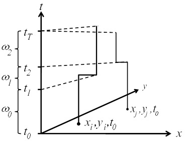
3.1. Space-Time Analysis
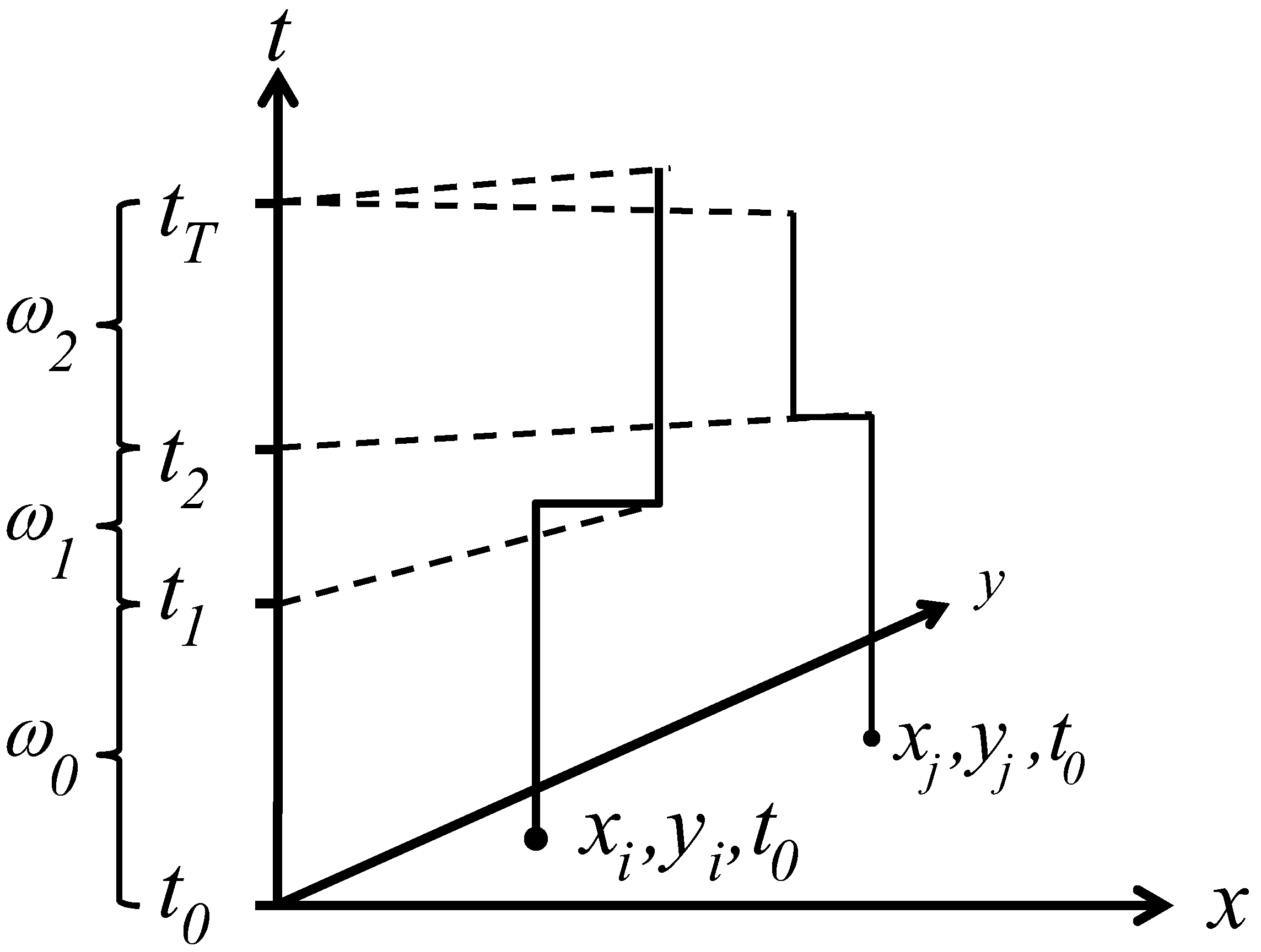
3.2. Ǫ-Statistics
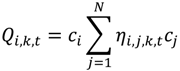
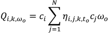
3.2.1. A Diagnostic Framework for Ǫ-Statistics in Relation to Disease Processes

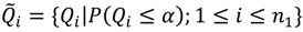

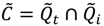
 is the set of all Ǫit that are statistically significant at the type I error level α, Ǫi,
  is the set of all Ǫi that are statistically significant at α, and
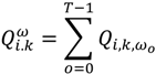
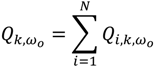
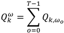
  is the set of all Ǫt that are statistically significant at α. It turns out that Ǫt and Ǫi are global statistics that assess case-clustering at specific times (e.g., Ǫt) and over the life course of specific cases (e.g., Ǫi) such that:
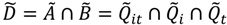
 and . This mapping is comprised of those Ǫit that contribute to the significant (through Equation (9)) and those Ǫit that contribute to the significant (through Equation (10)). Understanding this allows for the consideration of the following operations:
3.2.2. Assessing Overall Significance of Cluster Types
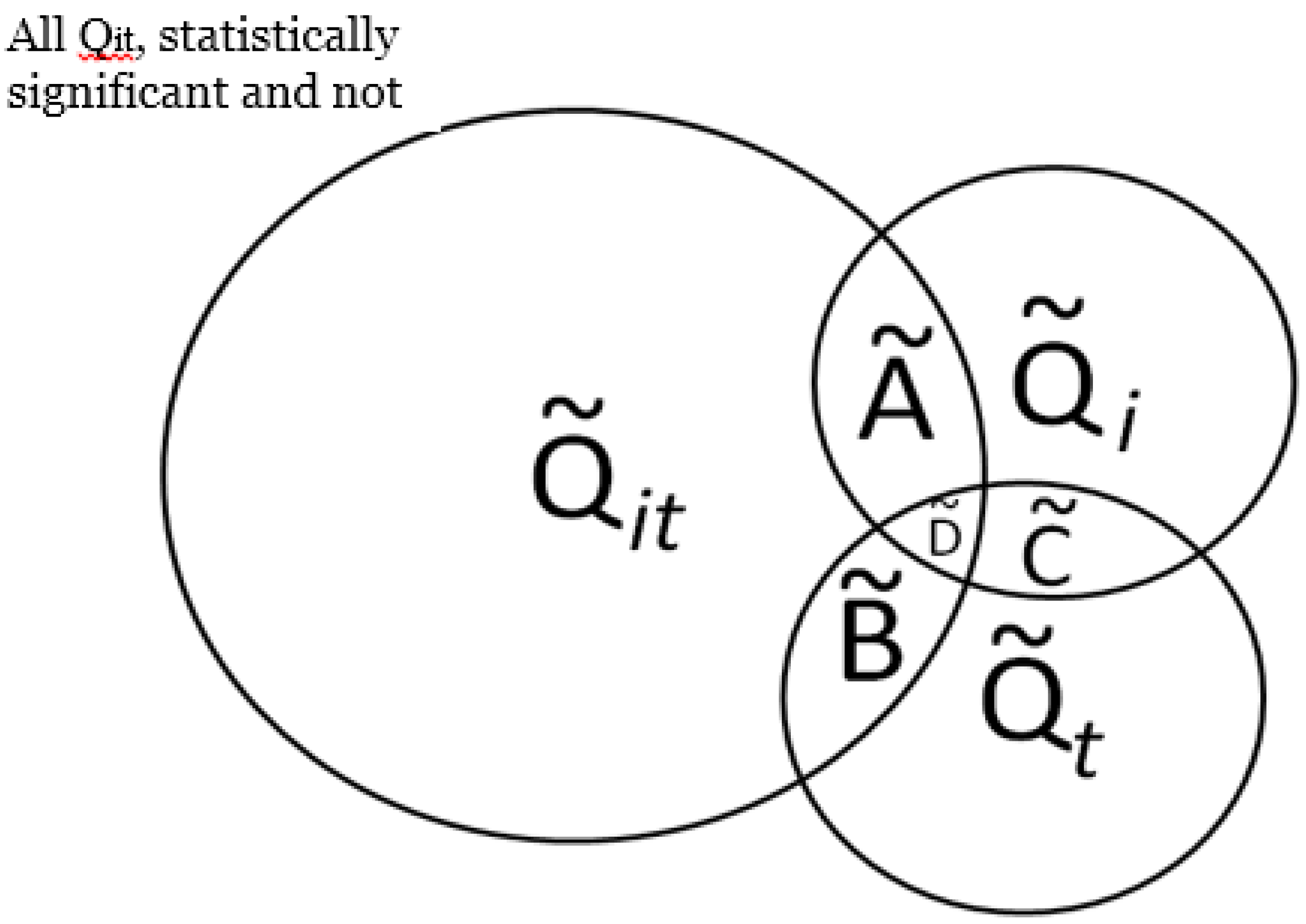
), over a cases’ life course (e.g., excess of cases about the residential history of case i, ), and globally at a given time t when all cases are considered together (e.g., large-scale spatial clusters at time t, ). These cluster sets and their intersections (Ã,  ,
,  ,
,  ) can provide insights into, and generate hypotheses regarding, disease etiologies. When the underlying Ǫ-statistics have been adjusted for the risk factors and covariates found significant in the parent case-control study these cluster types identify where, when, and to whom to allocate unexplained (e.g., excess) risk (Table 1).
), over a cases’ life course (e.g., excess of cases about the residential history of case i, ), and globally at a given time t when all cases are considered together (e.g., large-scale spatial clusters at time t, ). These cluster sets and their intersections (Ã, , , ) can provide insights into, and generate hypotheses regarding, disease etiologies. When the underlying Ǫ-statistics have been adjusted for the risk factors and covariates found significant in the parent case-control study these cluster types identify where, when, and to whom to allocate unexplained (e.g., excess) risk (Table 1).
) can provide insights into, and generate hypotheses regarding, disease etiologies. When the underlying Ǫ-statistics have been adjusted for the risk factors and covariates found significant in the parent case-control study these cluster types identify where, when, and to whom to allocate unexplained (e.g., excess) risk (Table 1).
), over a cases’ life course (e.g., excess of cases about the residential history of case i, ), and globally at a given time t when all cases are considered together (e.g., large-scale spatial clusters at time t, ). These cluster sets and their intersections (Ã, , , ) can provide insights into, and generate hypotheses regarding, disease etiologies. When the underlying Ǫ-statistics have been adjusted for the risk factors and covariates found significant in the parent case-control study these cluster types identify where, when, and to whom to allocate unexplained (e.g., excess) risk (Table 1). . The number of elements in this set,
  , in a setting where true clustering exists, is comprised of both true positives and false positives (call this
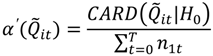
  . If it is possible evaluate the probability of under the null hypothesis of random labeling of the residential histories as cases or controls, and conditioned by the observed number of cases and controls, it is also possible to evaluate the significance of the cluster types in Figure 2 with a single test. In other words, the purpose is to assess the probability of observing the number of elements in the set . Table 2 enumerates the test statistics to be assessed, the cluster types they correspond to, and the probabilities to be evaluated.
| Cluster set | Description | Pattern | Possible etiology |
|---|---|---|---|
| | Cases (i) that at times t have a significant number of nearest neighbors that are cases | Cases (i) that at times t have a significant number of nearest neighbors that are cases. | Infection: Contagious process such that infection spreads from a case to its susceptible neighbors. Vector-borne disease process such that individuals in specific areas have increased risk of infection. Chronic (e.g., cancer): Increased cancer risk for individuals residing in local areas over a defined time period. Duration of elevated risk must be sufficiently long relative to the duration of time individuals live in the affected areas (e.g.,) exposure time must be sufficient to induce disease response. |
| | Clustering over the life course | Cases (i) who, over the study, have a significant number of nearest neighbors that are cases. | Infection: The “typhoid Mary” or “super-spreader” process, whereby case (i) (the super-spreader) is infectious over the study period and transmits infections to nearest neighbors. Chronic (e.g., cancer): A process whereby neighbors of case i have increased cancer risk and such risk is elevated over the life course of case i. An example would be behaviors that increase cancer risk for others such as second hand smoke. May also arise when groups with elevated risk tend to move or remain together over their life course (e.g., familial groups with common genetic and/or behavioral risk factors). |
| | Temporal case clustering | Large scale spatial clustering of cases at time t. Clustering of cases relative to controls is significant at time t when all cases and controls are considered. | Infection: Infection outbreak such that the infection impacts a large portion of the study population; endemic phase of infection with multiple local outbreaks. Chronic (e.g., cancer): Chronic disease with an underlying infectious etiology (e.g., viral hypothesis of cancer) that impacts a large portion of the study participants; Disease risk mediated by environmental exposures that vary across the study area such that risk is elevated for a large number of study participants. Duration of elevated risk must be sufficiently long relative to the duration of time individuals live in the affected areas (e.g., exposure time must be sufficient to induce disease response). |
| Ã |  | Locations and time when cases with significant clustering over their life course are members of a geographically localized cluster. Includes both ephemeral and persistent clusters. | Infection: Local foci of infection occurring at times t from which infected and infectious cases move away. Chronic (e.g., cancer): Local areas of persistent elevated risk that are sustained for a sufficient period of time that (1) disease risk is increased for individuals residing in the local area and (2) the duration of residence of cases in the area is of sufficient length to result in a significant Ǫi statistic. |
| |  | Cases (i) who, over the study, have a significant number of nearest neighbors that are cases. | Infection: Large-scale outbreak at specific times, t, that may be comprised of local pockets of infection. For vector-borne diseases this can arise when large portions of the study area have suitable vector habitat during some parts of the study period. Chronic (e.g., cancer): Large scale exposures that occur at a specific time(s) t. An example would be leukemia in response to the Chernobyl and Hiroshima incidents. |
| | | Cases that have clustering over their life course and are part of large-scale spatial clusters at times t. Includes cases whose Ǫit are not statistically significant, and some whose Ǫit are statistically significant. | Infection: Large-scale outbreak at times t with at least some of the resulting cases that (1) move together over their life course; and/or (2) remain infectious over their life course and continue to infect their neighbors. For a vector-borne disease this may arise when there is an initial large scale outbreak with some of the resulting cases continuing to be disease reservoirs (e.g., pathogen sources) whose infection can then be transmitted to neighbors. Behavioral: Individuals who have a behavior link that causes them to be at an increased exposure to an environmental factor, pathogen, or vector. The difference from Ǫi is that here, the exposure factor must temporally “outbreak” in nature in that it either cycles in population like a vector/pathogen can (such as bird flu) or in severity for an environmental factor. For example, imagine a poultry reseller who moves around. He has an elevated risk any time a bird flu epidemic breaks out so will show a Ǫi cluster and when the epidemics outbreak, there will be Ǫt clusters. An example would be where a pesticide is applied but because of laws is phased out, but later on people start using it again. Chronic (e.g., cancer): Large scale exposures that occur at a specific time(s) t with some of the resulting cases that (1) move together through life course or (2) continue to reside in the affected area over most of the study period. |
| |  | Cases that have clustering over their life course, are part of large scale clusters at time t and whose local clusters Ǫit are all statistically significant. | Etiology is similar to set , but is restricted to include only those individuals that are centers of significant local clustering of cases at times t. For infection, this may be indicative of index cases; for chronic diseases this may indicate individuals who are within local pockets of the largest exposure. |
| Cluster type | Cluster description | Test statistic | Probability of test statistic |
|---|---|---|---|
| | Local case-time | |  |
| | Life course |  |  |
| | Temporal case clustering |  |  |
| Ã | |  |  |
| | |  |  |
| |  |  |  |
| | |  |  |
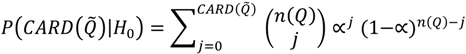
 is the probability of the cluster set denoted
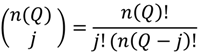
  under the null hypothesis; these correspond to the entries in the column “probability of test statistic” in Table 2. is the cluster set being considered; these are the entries in the column “Test statistic” in Table 2 and are the count of the number of significant clusters of that type. For example, recall that is the count of the number of observed cases that have significant clustering of cases about them over their life course. Here n(Ǫ) is the total number of occurrences of the statistic under consideration, whether significant or not. For example, n(Ǫi) = n1, where n2 is the number of cases in the study. Table 3 enumerates n(Ǫ) for the different cluster types. Finally,
  is the desired type I error of the test, often set to = 0.05.
| Cluster type | Cluster description | Test statistic | Number of possible elements in each set (n(Ǫ) in Equations (15) and (16)) |
|---|---|---|---|
| | Local case-time | |  |
| | Life course | | n1T |
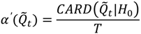
| | Temporal case clustering | | T |
3.2.3. Calculating the Empirical Type I Error under Multiple Testing
 is the number of false positives observed under the null hypothesis. The total number of possible tests as per Table 3 is , since the number of cases recorded in the data set will vary from one time to another, and since a local test is calculated for each case at each time point considered. The empirical type I error may then be estimated as:
 and as:
 that are observed for a given set (say
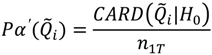
  ) under the null hypothesis using a specific type I error ( ) and number of simulation runs. This distribution is bounded on the right side by , and on the left side by
  , where nruns is the number of simulation runs conducted.
3.2.4. Adjusting Critical Values of the Test for Different Cluster Types
. Should this statistic prove significant (e.g.,  ), it is helpful to identify those Ǫ*i subsumed within the set
  that are likewise significant. This is a much smaller number than the maximum number of Ǫi that can be calculated, yet there is still a multiple testing issue.
3.3. Analysis Steps
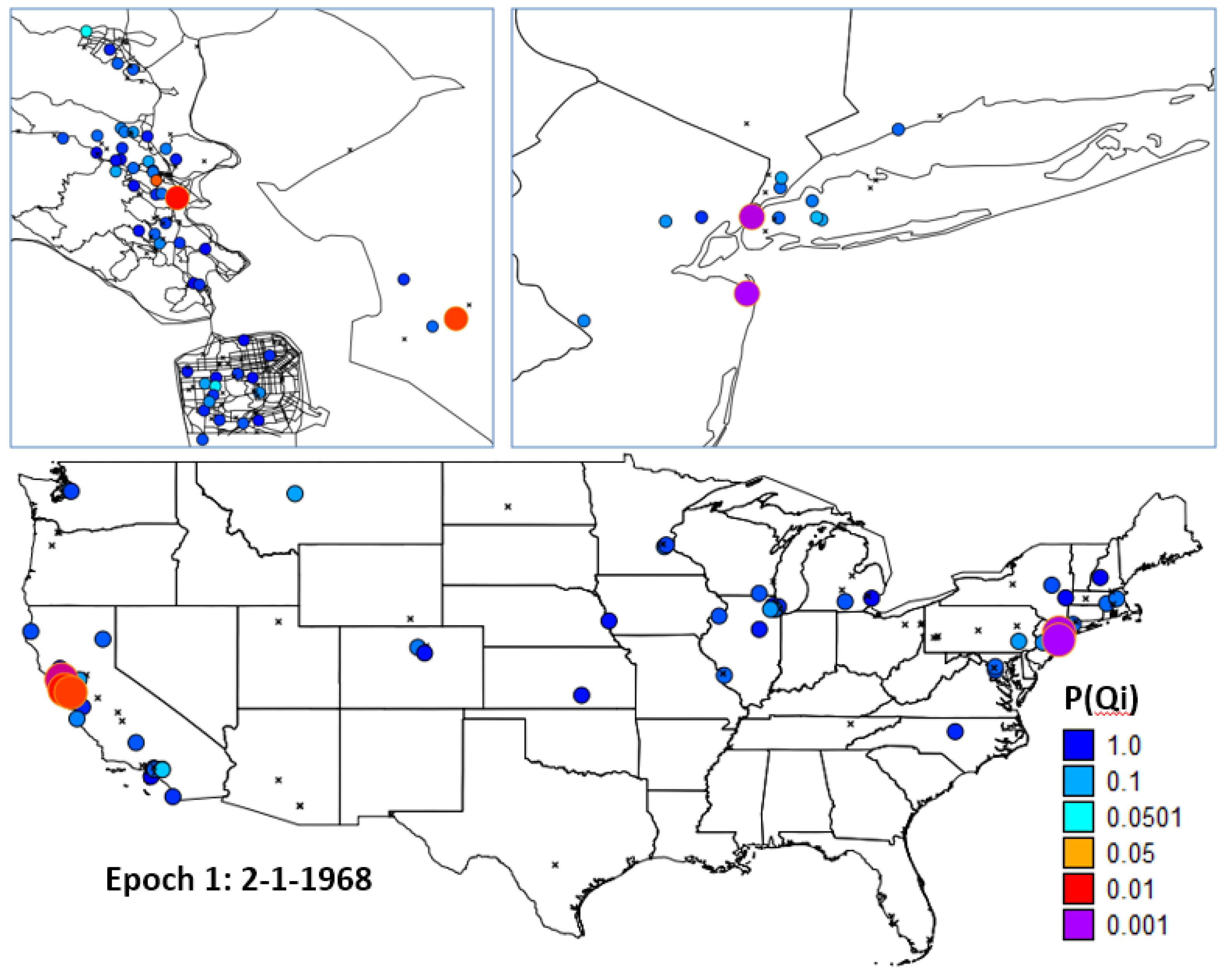
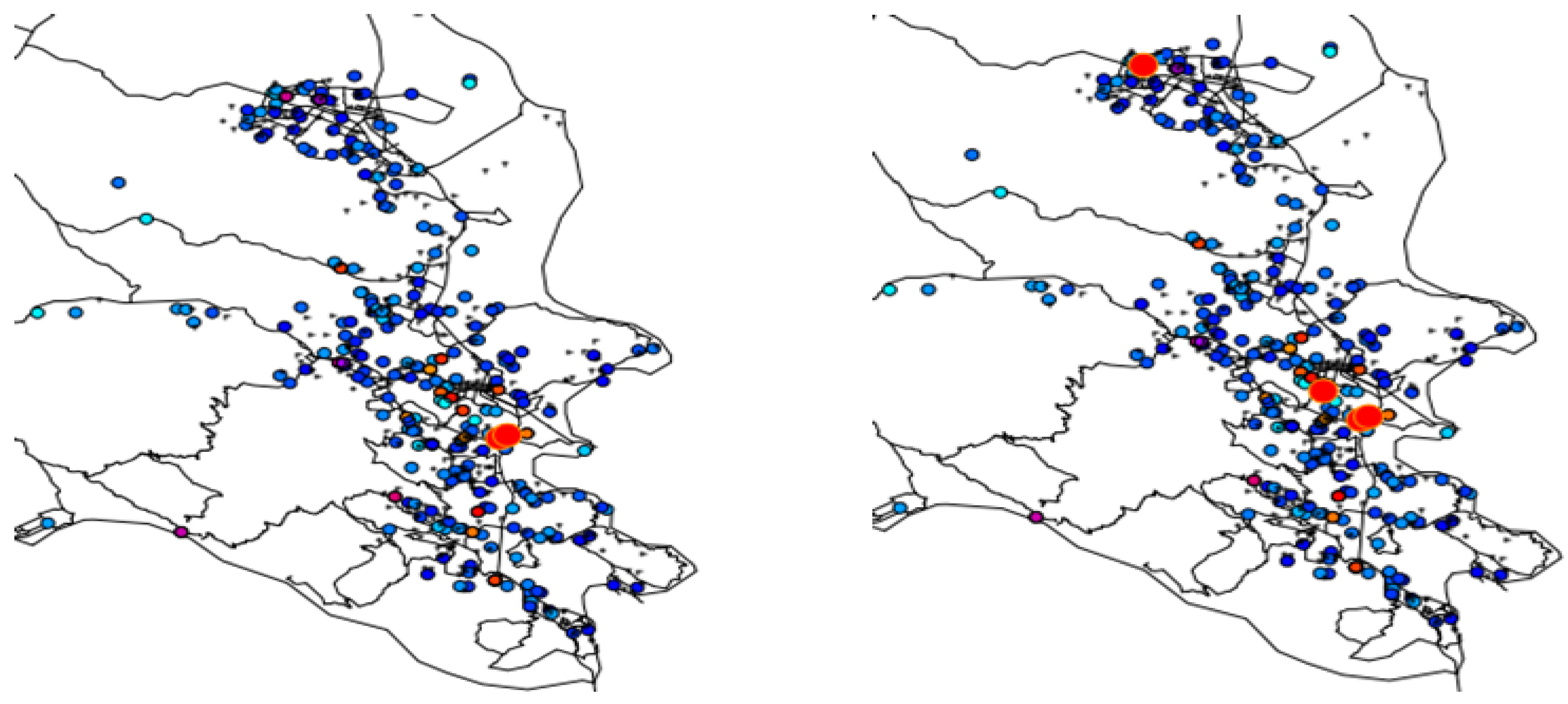
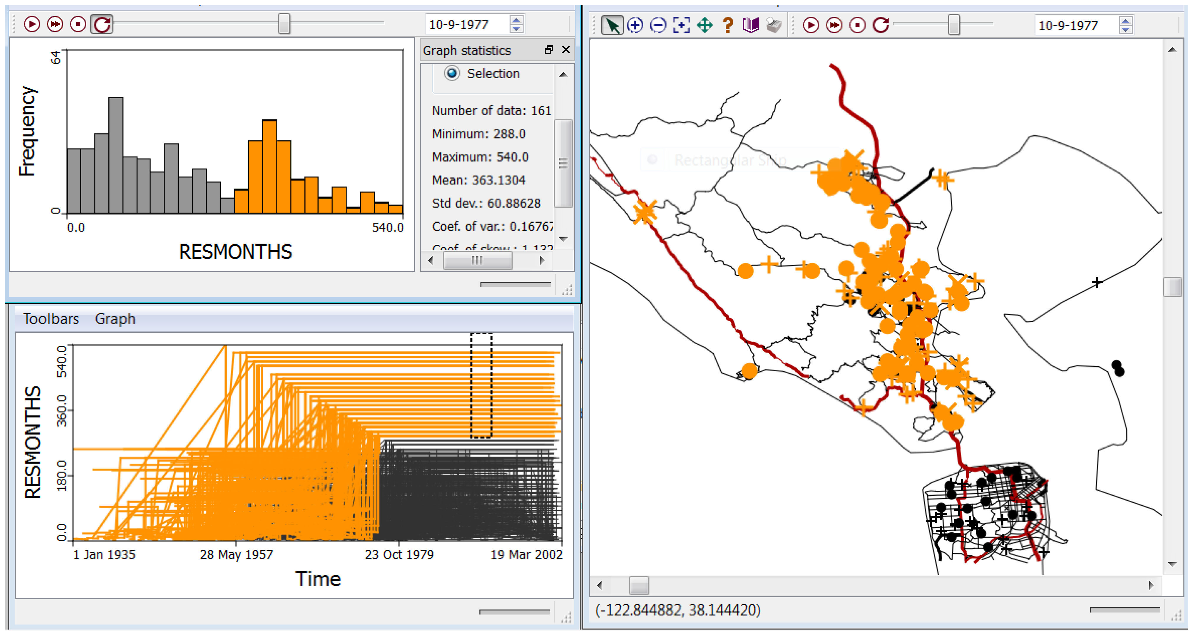
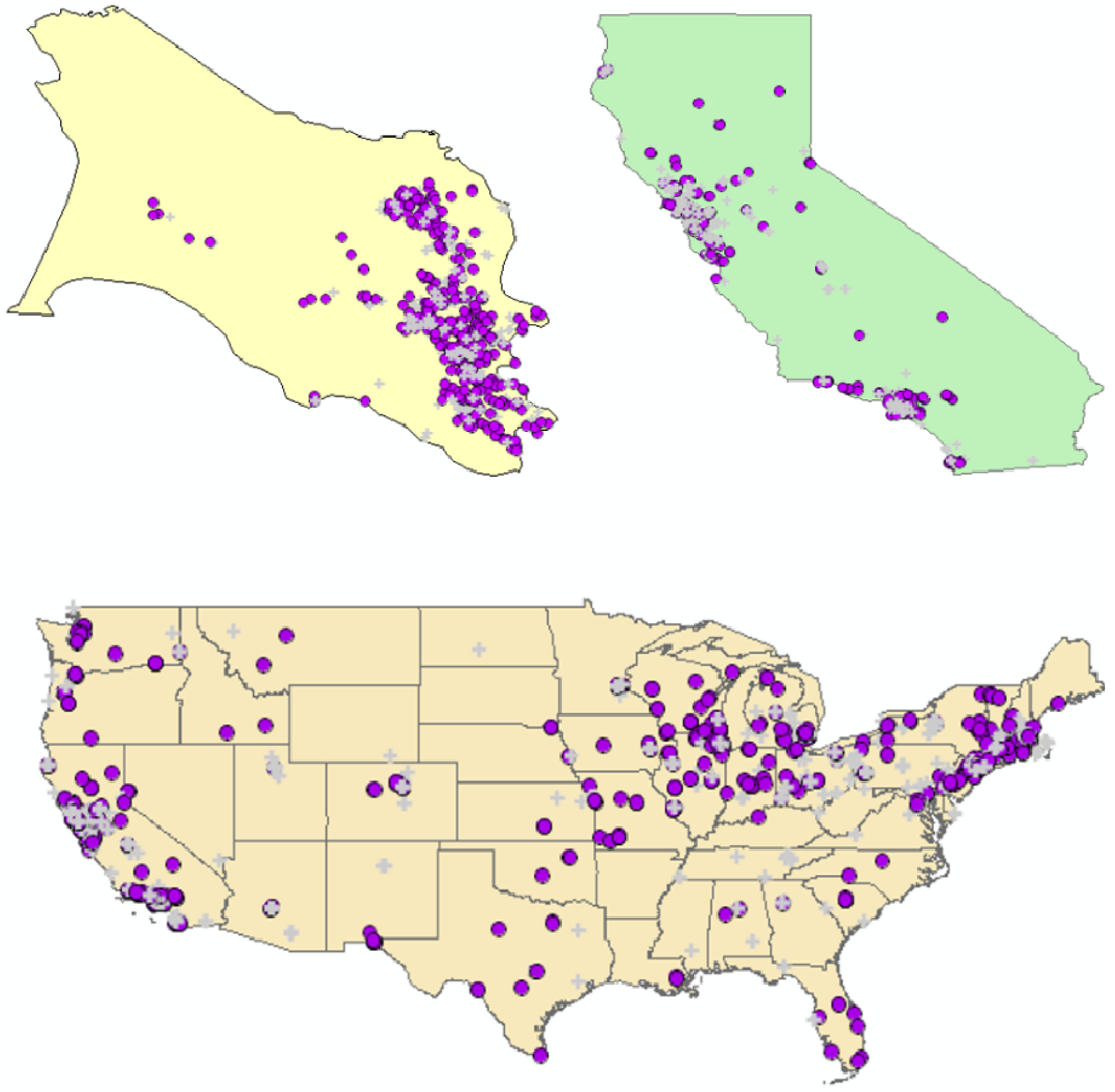
- H1: Evaluate residential mobility by mapping places of residence for the study participants at three spatial scales: Marin County, California, and the continental United States.
- H2: Evaluate global clustering over the entire study using the Global Ǫ-statistic.
- H3: Evaluate whether and when there are times that cases cluster relative to controls when all of the study participants are considered together using the Ǫt statistic.
- H4: Evaluate whether specific cases tend, over their life course, to have other neighbors as cases using the Ǫi statistic.
- H5: Using the significance of set A, evaluate whether cases that cluster over their life course (significant Ǫi) are part of local clusters at specific times (Ǫit).
4. Results
4.1. Geocoding
4.2. Hypotheses
4.2.1. H1: Cases and Controls Do not Exhibit Substantial Residential Mobility over the Life Course
4.2.2. H2: There Is No Statistically Significant Global Clustering of Breast Cancer Cases Relative to Controls When Accounting for Known Risk Factors and Covariates and for Residential Mobility

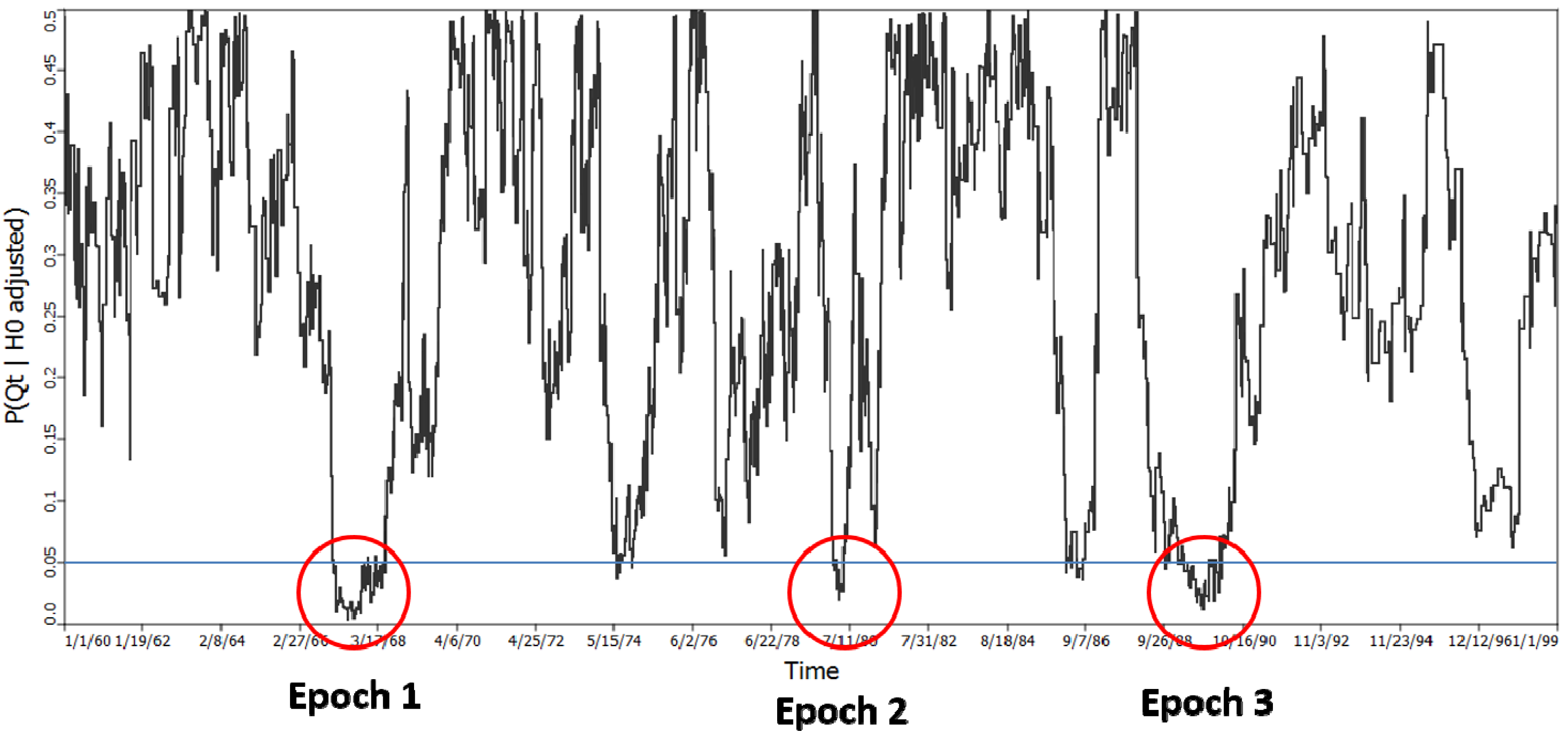
4.2.3. H3: There Are No Time Periods When the Breast Cancer Cases, Considered as a Group, Exhibit Statistically Significant Clustering Relative to the Controls
= 122, which yielded a probability of 0.000001625. This statistic is not subject to multiple testing, and indicates significant clustering of cases in some of the time periods considered. It does not however, identify when those time periods are, although they must be time periods from the set of 122. = 122 and is highly significant (p = 0.000001625).
= 122 and is highly significant (p = 0.000001625).
4.2.4. H4: Cases Do not Exhibit Statistically Significant Clustering over Their Life Course
) is itself statistically unusual. This second step has the advantage of not being subject to multiple testing, since only one measure ( ) is evaluated The test for Ǫi was performed using k = 5 and 999 randomization runs, while adjusting for the probability of being a case from the logistic regression in order to account for the risk factors and covariates found significant in the parent study by Wrensch et al. [5]. 30 cases were found to have significant clustering over their entire residential history. An evaluation of the probability of = 30 using the binomial expressions in Equations (15) and (16) yielded a probability of observing this outcome of p = 0.000115. 14.25 cases would have been expected to be significant at the nominal type I error of 0.05.4.2.5. H5: Cases that Cluster over the Life Course (Ǫi) Are not Part of Local Clusters at Specific Times (Ǫit)

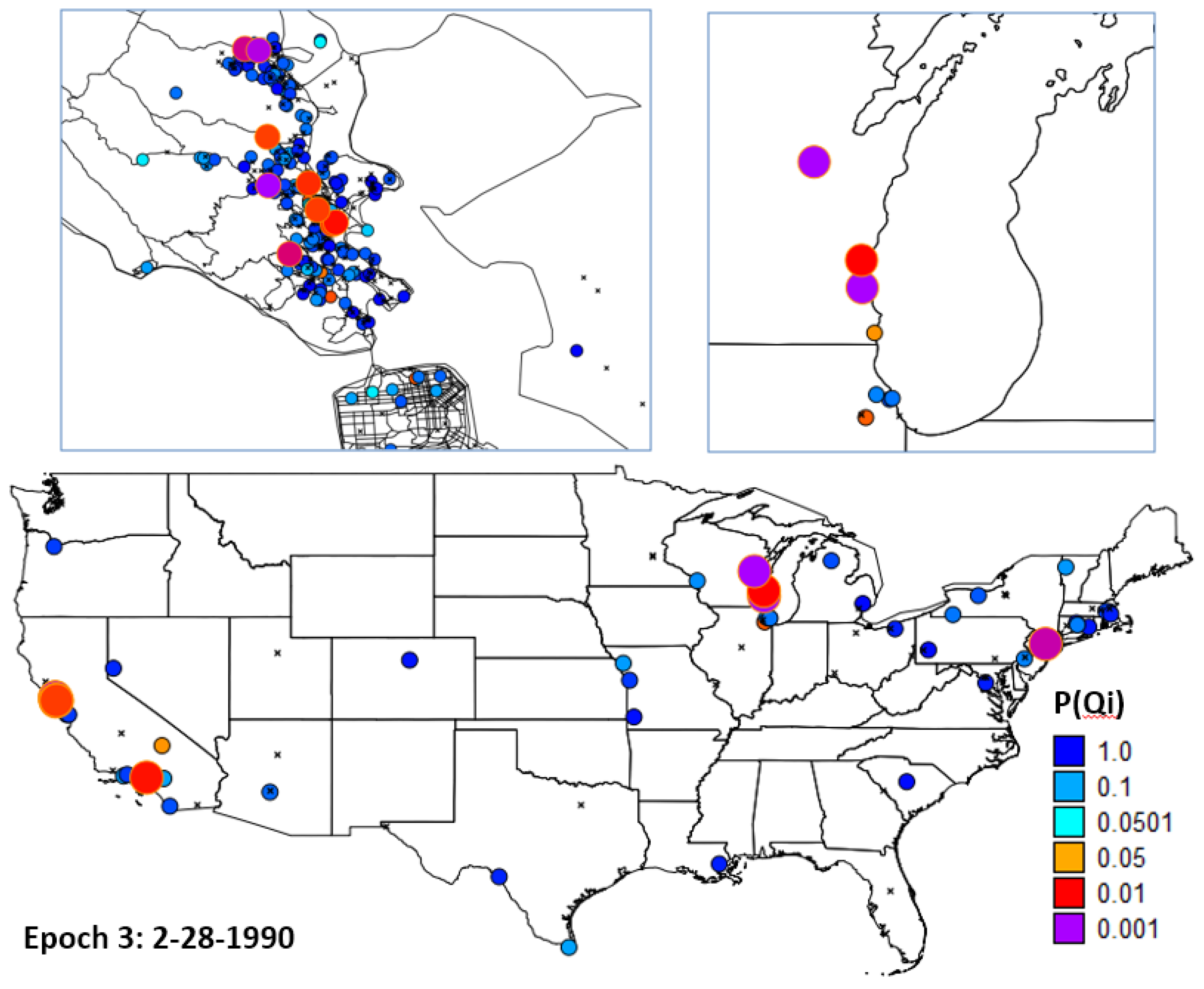
4.3. Synopsis and Synthesis: Locations of Persistent Life Course Clusters

5. Discussion
6. Conclusions
Acknowledgments
Conflicts of Interest
References
- Rothman, K.J.; Greenland, S.; Lash, T.L. Case-Control Studies. In Encyclopedia of Quantitative Risk Analysis and Assessment; Melnick, E.L., Everitt, B.S., Eds.; John Wiley Sons Ltd.: Chichester, UK, 2008; pp. 192–204. [Google Scholar]
- Jacquez, G.M.; Kaufmann, A.; Meliker, J.; Goovaerts, P.; AvRuskin, G.; Nriaqu, J. Global, local and focused geographic clustering for case-control data with residential histories. Environ. Health 2005, 4. [Google Scholar] [CrossRef] [Green Version]
- Vieira, V.; Webster, T.; Weinberg, J.; Aschnegrau, A. Spatial analysis of bladder, kidney, and pancreatic cancer on upper Cape Cod: An application of generalized additive models to case-control data. Environ. Health 8, 2009. [CrossRef]
- Rogerson, P.; Yamada, I. Statistical Detection and Surveillance of Geographic Clusters; CRC Press: New York, NY, USA, 2009. [Google Scholar]
- Wrensch, M.; Chew, T.; Farren, G.; Barlow, J.; Belli, F.; Clarke, C.; Erdmann, C.A.; Lee, M.; Moghadassi, M.; Peskin-Mentzer, R.; et al. Risk factors for brast cancer in a population with high incidence rates. Breast Cancer Res. 2003, 5, R88–R102. [Google Scholar] [CrossRef] [Green Version]
- Nuckols, J.; Airola, M.; Colt, J.; Johnson, A.; Schwenn, M.; Waddell, R.; Karagas, M.; Silverman, D.; Ward, M.H. The impact of residential mobility on exposure assessment in cancer epidemiology. Epidemiology 2009, 20, S259–S260. [Google Scholar]
- Jacquez, G.M. Space-Time Intelligence System Software for the Analysis of Complex Systems. In Handbook of Applied Spatial Analysis: Software Tools, Methods and Applications; Fischer, M., Getis, A., Eds.; Springer: New York, NY, USA, 2009; pp. 113–124. [Google Scholar]
- Jacquez, G.M.; Meliker, J.R.; AvRuskin, G.A.; Goovaerts, P.; Kaufmann, A.; Wilson, M.L.; Nriagu, J. Case-control geographic clustering for residential histories for epidemiologic studies. Int. J. Health Geogr. 2006, 5. [Google Scholar] [CrossRef]
- Hochberg, Y. A sharper Bonferroni procedure for multiple test of significance. Biometrika 1988, 75, 800–802. [Google Scholar] [CrossRef]
- Hommel, G. A stagewise rejective multiple test procedure based on a modified Bonferroni test. Biometrika 1988, 75, 383–386. [Google Scholar] [CrossRef]
- Simes, R.J. An improved Bonferroni procedure for multiple tests of significance. Biometrika 1986, 73, 751–754. [Google Scholar] [CrossRef]
- Benjamini, Y.; Hochberg, Y. Controlling the false discovery rate: A practical powerful approach to multiple testing. J. R. Stat. Soc. Ser. B 1995, 57, 289–300. [Google Scholar]
- Storey, J.D.; Tibshirani, R. Statistical significance for genomewide studies. Proc. Natl. Acad. Sci. USA 2003, 100, 9440–9445. [Google Scholar] [CrossRef]
- Jacquez, G.M.; Slotnick, M.J.; Meliker, J.R.; AvRuskin, G.; Copeland, G.; Nriagu, J. Accuracy of commercially available residential histories for epidemiologic studies. Am. J. Epidemiol. 2011, 173, 236–243. [Google Scholar] [CrossRef]
- Meliker, J.R.; Jacquez, G.M. Space-time clustering of case-control data with residential histories: Insights into empirical induction periods, age-specific susceptibility, and calendar year-specific effects. Stoch. Environ. Res. Risk Assess. 2007, 21, 625–634. [Google Scholar] [CrossRef]
© 2013 by the authors; licensee MDPI, Basel, Switzerland. This article is an open access article distributed under the terms and conditions of the Creative Commons Attribution license (http://creativecommons.org/licenses/by/3.0/).
Share and Cite
Jacquez, G.M.; Barlow, J.; Rommel, R.; Kaufmann, A.; Rienti, M., Jr.; AvRuskin, G.; Rasul, J. Residential Mobility and Breast Cancer in Marin County, California, USA. Int. J. Environ. Res. Public Health 2014, 11, 271-295. https://doi.org/10.3390/ijerph110100271
Jacquez GM, Barlow J, Rommel R, Kaufmann A, Rienti M Jr., AvRuskin G, Rasul J. Residential Mobility and Breast Cancer in Marin County, California, USA. International Journal of Environmental Research and Public Health. 2014; 11(1):271-295. https://doi.org/10.3390/ijerph110100271
Chicago/Turabian StyleJacquez, Geoffrey M., Janice Barlow, Robert Rommel, Andy Kaufmann, Michael Rienti, Jr., Gillian AvRuskin, and Jawaid Rasul. 2014. "Residential Mobility and Breast Cancer in Marin County, California, USA" International Journal of Environmental Research and Public Health 11, no. 1: 271-295. https://doi.org/10.3390/ijerph110100271