An Environmental and Economic Evaluation of Pyrolysis for Energy Generation in Taiwan with Endogenous Land Greenhouse Gases Emissions

Abstract

Taiwan suffers from energy insecurity and the threat of potential damage from global climate changes. Finding ways to alleviate these forces is the key to Taiwan’s future social and economic development. This study examines the economic and environmental impacts when ethanol, conventional electricity and pyrolysis-based electricity are available alternatives. Biochar, as one of the most important by-product from pyrolysis, has the potential to provide significant environmental benefits. Therefore, alternative uses of biochar are also examined in this study. In addition, because planting energy crops would change the current land use pattern, resulting in significant land greenhouse gases (GHG) emissions, this important factor is also incorporated. Results show that bioenergy production can satisfy part of Taiwan’s energy demand, but net GHG emissions offset declines if ethanol is chosen. Moreover, at high GHG price conventional electricity and ethanol will be driven out and pyrolysis will be a dominant technology. Fast pyrolysis dominates when ethanol and GHG prices are low, but slow pyrolysis is dominant at high GHG price, especially when land GHG emissions are endogenously incorporated. The results indicate that when land GHG emission is incorporated, up to 3.8 billion kWh electricity can be produced from fast pyrolysis, while up to 2.2 million tons of CO₂ equivalent can be offset if slow pyrolysis is applied.

1. Introduction

Taiwan is heavily reliant on imported fossil fuels. To enhance energy security, there is interest in domestic energy production. Climate change is also a concern for Taiwan with defenseless warming, sea level rises and increased incidence of tropical cyclones [1]. Energy based CO₂ emissions could be a driving force for these disasters [1]. Collectively these forces have raised interest in examining low emission, domestic energy sources. Renewable energy produced from agricultural feedstocks (hereafter called bioenergy) is one such possibility.

Bioenergy production requires substantial use of land resources, another scarce resource in Taiwan. However, after joining the World Trade Organization (WTO), 280,000 hectares of Taiwan’s agricultural land were idled due to reductions in subsidies and increases in imports. This provides some land that could be used for bioenergy feedstock production.

Although bioenergy has the potential to enhance Taiwan’s energy security and reduce its GHG emissions [2], one important factor that may affect the net benefits is the total set of land and other based GHG emissions involved with feedstock production. When agricultural land is converted to other uses, N₂O emissions will change and offset CO₂ energy related emission reductions. If the change is small this can be neglected. Unfortunately, this change can be large [3,4]. For this reason, endogenous incorporation of land GHG emissions could have a significant impact on bioenergy production and emissions reduction.

Therefore, examining the desirability of bioenergy production without considering all GHG emissions may lead to an incorrect conclusion. This study examines the economic and environmental performance of a set of bioenergy production strategies including production of ethanol, direct firing of electricity production and pyrolysis-based electricity. They will be evaluated under a range of energy and GHG prices. Performance will be considered in terms of GHG emissions, energy production and economic implications. The work will simultaneously consider multiple bioenergy technologies, multiple energy crops, multiple energy and GHG prices, alternative uses of products from pyrolysis and CO₂ emissions from land use change.

2. Literature Review

Taiwan can produce bioenergy in the forms of bioethanol, direct feedstock combustion biopower (conventional electricity) and biopower using products produced through pyrolysis (pyrolysis-based electricity). Since these three technologies are not mutually exclusive and can be employed at the same time, the study considers all combinations.

Pyrolysis involves heating biomass in the absence of oxygen and results in the decomposition of the biomass into biooil, biogas and biochar, all of which can be used to generate electricity. Depending on the heating rate and time staying in the machine, pyrolysis could be categorized as fast pyrolysis and slow pyrolysis. The main difference between fast and slow pyrolysis is that fast pyrolysis yields more biooil, while slow pyrolysis yields more biochar [5,6]. Biochar can be used as an energy source or as a soil amendment [7,8,9,10,11]. As a soil amendment biochar increases soil water and nutrient holding capacity plus seed germination rates and crop yields. In terms of water holding capacity, Glaser et al. [12] find that soil water retention increased by 18% after biochar application. In terms of nutrient savings, the application of biochar has been found to increase the efficiency of nutrients as discussed in Steiner et al. [13]. Lehmann et al. [14] also indicates that biochar application would lead to a reduction of N leaching by 60 percent with an accompanying 20% savings in fertilizer need. On seed germination several studies find that biochar improves seed germination rate [15,16]. In terms of crop yield enhancement, Lehmann [8] finds that biochar increases the plants available nutrients and in turn crop yields. Crop yield increases have also been found by [13,17,18,19,20] with yield increases ranged from 44% to 249%. Nehls [21] finds rice yield increases ranging from 115% to 320%. Biochar is also stable in the soil [13] and offers a chance to sequester carbon [8].

Based on these data we assume that rice yields will increase by 5% when biochar is applied and use that the seed and nutrient savings are based on Lehmann et al.’s study [13] (20 and 10 %, respectively) while water savings are assumed to be 10%. In addition, since water is usually produced during pyrolysis and reduces the heating value, so it is important to remove water from the liquid content. Since electricity and biochar production vary depending on the pyrolysis systems, we examine fast and slow forms of pyrolysis techniques and alternatives uses of biochar.

Lifecycle analysis [22] has been used to examine GHG emissions from agriculture and bioenergy production in a number of settings. Schaufler et al. [23] showed that changes in land-use strongly affected GHG fluxes from cropland, grassland, forests and wetland. Grover et al. [4] pointed out that soil-based GHG emissions increase from 53 to 70 t CO₂-equivalents after land use change. They found that N₂O and CO₂ emissions were highest from grassland soils. Baldos [24] found that the direct lifecycle GHG emissions of corn ethanol fuel can exceed the 20% GHG reduction requirement in the USA renewable fuel standard. Baggs et al. [25] found that zero tillage resulted in higher N₂O emissions than conventional tillage and N₂O emissions were generally correlated with CO₂ emissions. Farquharson and Baldock [26] indicated that adding N fertilizers will increase N₂O emissions due to nitrification and denitrification process. Wang et al., [27] and Searchinger et al. [28] examined the impacts of emissions from global land use changes finding they can substantially offset GHG net emission gains. Other studies have focused on the land use change emissions when specific land types are cultivated for cropland use [29,30,31].

3. Model Structure

The study will be done using an agricultural sector model. The model used herein is based on price endogenous mathematical programming, which is originally illustrated by Samuelson [32] who showed a perfectly competitive equilibrium can be simulated by solving an optimization model that maximizes the consumers’ plus producers’ surplus. In particular we will use Chen and Chang’s [33] Taiwan Agricultural Sector Model (TASM) that we extend TASM to cover bioenergy crop production.

The TASM is a multi-product partial equilibrium model based on the previous work [34,35,36,37]. TASM has been used in many policy-related studies such as Chang [36] and Chen and Chang [33]. The current version covers production in 15 subregions aggregated into four major market regions. It incorporates price-dependent product demand for 60 traditional crops, five floral crops, seven livestock species, three types of forests (conifers, hardwoods, and bamboo), and 27 secondary commodities. The total value of these primary commodities accounts for more than 85 percent of Taiwan’s total agricultural product value. Availability of cropland, pasture land, set aside and forest land plus crop and livestock mix constraints are specified at the sub-regional level. Input markets for farm labor are specified at the regional level with supply curves.

3.1. Modified Taiwan Agricultural Sector Model

For this analysis we extend the TASM version of Chen and Chang [33] adding features related to farm support, bioenergy and GHG emissions. The algebraic form of the modified TASM is as follows:

(1)

subject to:

(2)

Σ_iX_ik + AL_k + Σ_jEC_jk - L_k≤0 for all k,

(3)

Σ_if_ikX_ik - Σ_jf_jkX_jk - R_k≤0 for all k,

(4)

Σ_i,kE_gikX_ik-Baseline_g = GHG_g for all g

(5)

Equation (1) is the objective function. The area under the domestic demand curve is the 1st term while input costs are in the 2nd term. Then the area under the cropland and labor supply curves are in the 3rd and 4th terms, respectively. The 5th, 6th and 7th terms reflect the government subsidies on rice purchase, set-aside lands and the planting of energy crops. The 8th and 9th terms represent the area under the rest of world export excess demand curve and the 10th term stands for the area under the rest of world excess supply curve. The 11th term is tariff revenue. The final term models GHG offset payments under a carbon dioxide equivalent price.

Equation (2) is the balance constraint for commodities. The first three terms give alternative demands which includes domestic demand (Q_i), export demand (Q_i^X), and government purchases (Q_i^G). The last two terms in the supply-demand balance constraint represents the supply side and include domestic production (Σ_kY_ikX_ik) and imports (Q_i^M + TRQ_i). Table 1 depicts the details of variables.

Table 1. Variables and their descriptions.

Qi	Domestic Demand of Product
QiG	Government purchases quantity for price supported product
QiM	Import quantity of product
QiX	Export quantity of product
ψ(Qi)	Inverse demand function of product
PiG	Government purchase price on product
Cik	Purchased input cost in region for producing product
Xik	Land use for commodities produced in region
Xjk	Land use for energy crop produced in region
Lk	Land supply in region
αk(Lk)	Land inverse supply in region
Rk	Labor supply in region
βk(Lk)	Labor inverse supply in region
PL	Set-aside subsidy
ALk	Set-aside acreage in region
SUBj	Subsidy on planting energy crop
ECjk	Planted acreage of energy crop in region
ED(QiM)	Inverse excess import demand curve for product
ES(QiX)	Inverse excess export supply curve for product
TRQi	Import quantity exceeding the quota for product
EXED(TRQi)	Inverse excess demand curve of product that the import quantity is exceeding quota
taxi	Import tariff for product
outtaxi	Out-of-quota tariff for product
Yik	Per hectare yield of commodity produced in region
Egik	greenhouse gas emission from product in region
PGHG	Price of GHG gas
GWPg	Global warming potential of greenhouse gas
GHGg	Net greenhouse gas emissions of gas
Baselineg	Greenhouse gas emissions under the baseline of the gas

Table 1. Variables and their descriptions.

Qi	Domestic Demand of Product
QiG	Government purchases quantity for price supported product
QiM	Import quantity of product
QiX	Export quantity of product
ψ(Qi)	Inverse demand function of product
PiG	Government purchase price on product
Cik	Purchased input cost in region for producing product
Xik	Land use for commodities produced in region
Xjk	Land use for energy crop produced in region
Lk	Land supply in region
αk(Lk)	Land inverse supply in region
Rk	Labor supply in region
βk(Lk)	Labor inverse supply in region
PL	Set-aside subsidy
ALk	Set-aside acreage in region
SUBj	Subsidy on planting energy crop
ECjk	Planted acreage of energy crop in region
ED(QiM)	Inverse excess import demand curve for product
ES(QiX)	Inverse excess export supply curve for product
TRQi	Import quantity exceeding the quota for product
EXED(TRQi)	Inverse excess demand curve of product that the import quantity is exceeding quota
taxi	Import tariff for product
outtaxi	Out-of-quota tariff for product
Yik	Per hectare yield of commodity produced in region
Egik	greenhouse gas emission from product in region
PGHG	Price of GHG gas
GWPg	Global warming potential of greenhouse gas
GHGg	Net greenhouse gas emissions of gas
Baselineg	Greenhouse gas emissions under the baseline of the gas

Equations (3) and (4) are the resource endowment constraints. Equation (3) controls cropland insuring that planted land plus set-aside land cannot exceed total land and reflects competition by agricultural crops, energy crops and set-aside hectares. Equation (4) is the constraint for other resources such as fertilizer, irrigation and labor requirement. Equation (5) is the net greenhouse gas balance which accounts for the net gain in emissions relative to the baseline as in McCarl and Schneider [38].

3.2. Modeling Farm Support Policy

In order to incorporate ongoing domestic policies that support rice prices and set-aside cropland, the modified TASM required the addition of variables that reflected the government rice purchasing program and the set-aside program. The rice purchasing program provides farmers with a guaranteed price that is higher than the market equilibrium price. Letting P_i^G be the weighted government guaranteed purchase price and Q_i^G be the total amount of government purchase. The farm revenue realized from the government rice purchase program is added into the objective function as an additional farm revenue source. At the same time, it removes rice from the market place up to the amount allowed.

The other set of policy variables related to the land set-aside program are discussed next. If farmers choose to participate in this program, then those farmers will receive a set-aside payment (P^L). The purpose of the objective function that includes consumer and producer surplus is to derive the equilibrium under a perfectly competitive market. We add the government expenditure to the objective function; however, this does not mean that we treat the government expenditure as social welfare; instead, it reflects the distorted demand function.

3.3. Modeling Energy Crops and Conversion

Production activities for raising sweet potatoes, poplar and switchgrass as bioenergy feedstocks plus their conversion into ethanol and electricity are incorporated into the modified TASM. Here we discuss that modeling.

First, under current policy there is a substantial amount of set-aside land and these crops are modeled as using that land. Second in terms of crops sweet potatoes are currently produced in Taiwan, but not poplar and switchgrass. For this reason, input costs and yields for those crops are obtained from the literature and established models. Aylott et al. [39] showed that the yield of poplar is generally from 5.77 to 9.59 t/ha per year and this difference is caused by the quality of soil at the plantation and local weather. Sandy soil usually has the lowest yield. Since soil on Taiwan set-aside land is not sandy, this study takes average poplar yield. Switchgrass is a robust lowland energy crop most suited to the southern USA and has been tested in Auburn University test plots. In general, it has produces more than 10 tons per acre per year. Some U.S. government projects show that the yield of switchgrass is between 2 and 4 tons per acre per year and therefore, to be conservative, we use the average yield from government studies in our analysis. Since 1 hectare is 2.471 acres, the assumed annual yield of switchgrass is 3 × 2.471 = 7.4 t/ha per year.

Third, in terms of transformation to energy ethanol and electricity transformations are included in the model (in US dollars). For sweet potato, we added a facility construction cost of NT$2.4 per liter and a processing cost of NT$8.4 per liter. We also added a hauling cost of NT$1 per liter of ethanol that was estimated following McCarl et al.’s 2000 [40] hauling cost formula. For poplar and switchgrass, ethanol cost data is from FASOM [41]. After adjusting for Taiwanese consumer price index, the processing cost (including fixed cost, hauling cost and other costs) is NT$12 per liter for poplar and NT$11 per liter for switchgrass. Since poplar and switchgrass are not planted in Taiwan, elasticities of demand are set equal to the elasticity of hardwood varieties. Outputs are calculated based on the data of Aylott et al. [39] while production costs are calculated based on the information from FASOMGHG [42]. Fertilizer and chemical costs per hectare are calculated to NT$11,885 for poplar and $18,763 for switchgrass. Per hectare energy and seed costs are calculated to NT$706 and NT$5,410 for poplar and NT$488 and NT$306 for switchgrass, respectively. We also compute the net mitigation of carbon dioxide using an estimate from Weber and Johannes [43]. They show that net carbon dioxide emissions are reduced by 0.107 ton per 1,000 liters of ethanol. Electricity generated from a kg of poplar is about 0.768 kWh and 0.919 kWh per kg for switchgrass. Therefore, a kg of poplar and switchgrass are equivalent to 0.125 kg and 0.149 kg of coal, respectively. McCarl [44] estimates that poplar can offset about 71.3% of carbon dioxide emissions relative to the fossil fuel, 83.4% and 75.1% for switchgrass and the associate emissions reduction is 0.28 kg CO₂ per kg of poplar and 0.246 kg CO₂ for switchgrass.

3.4. Modeling Pyrolysis and Biochar

In this study, sweet potato, poplar and switchgrass are examined as potential pyrolysis feedstocks. Pyrolysis yields biooil, biogas and biochar. Following McCarl et al. [11] biooil and biogas are modeled as being used for bioelectricity generation, while biochar has multiple uses. First, biochar can be burned to provide electricity and reduce production cost. Second, biochar can be applied on cropland and obtain agricultural benefits such as higher crop yields and lower irrigation water use.

Table 2 shows the pyrolysis outputs for sweet potato, poplar and switchgrass. The pyrolysis yields for sweet potato we used in this study are based on He et al. [45]. Pyrolysis yields of poplar are based on Bridgwater and Peacocke [46]. Because we analyze the different uses of biochar, the net electricity produced from pyrolysis will be different if biochar is not used for electricity generation. Data from Table 2 is further processed to remove water content from biooil, which better simulate the net electricity production. The lower heating value of the biochar, biooil and biogas are taken as 11.4 MJ per kg [11], 17.3 MJ per kg and 6.5 MJ per kg [47], respectively. By using these estimates, we calculate the electricity generated from the pyrolysis of each energy crop.

Table 2. Outputs from Fast and Slow Pyrolysis.

Pyrolysis Type	Output	Poplar	Sweet Potato	Switchgrass
Fast Pyrolysis	Biooil	66%	87.56%	69%
	Biogas	13%	NA	11%
	Biochar	14%	12.44%	20%
Slow Pyrolysis	Biooil	56%	51.52%	58.55%
	Biogas	7%	34.99%	5.92%
	Biochar	31%	13.50%	44.29%

Source: [44,46].

Table 2. Outputs from Fast and Slow Pyrolysis.

Pyrolysis Type	Output	Poplar	Sweet Potato	Switchgrass
Fast Pyrolysis	Biooil	66%	87.56%	69%
	Biogas	13%	NA	11%
	Biochar	14%	12.44%	20%
Slow Pyrolysis	Biooil	56%	51.52%	58.55%
	Biogas	7%	34.99%	5.92%
	Biochar	31%	13.50%	44.29%

Source: [44,46].

3.5. Modeling GHG Emissions and Markets

The net GHG emissions offsets from pyrolysis, including both uses of biochar, are presented in Table 2. When burning biochar, all biochar is used to provide energy and therefore, we don’t need to consider hauling emissions. However, the GHG emissions offset from burning biochar in the pyrolysis plant as it displaces fossil fuels must be added. If biochar is used as a soil amendment, hauling is considered. Below presents the hauling cost for ethanol production. For sweet potatoes, we follow McCarl et al. [11] and assume that the ethanol plant is in the center of a square surrounded by a grid layout of roads. In turn, the hauling cost (H) and average hauling distance (D) is given by the following formula:

H = (b₀ + 2b₁D) S/Load

(6)

and:

(7)

where D is the average distance that the feedstock is hauled in miles; S is the amount of feedstock input for a bio-refinery to fuel the plant, which we assume is 1 Mt (annual input) plus an adjustment for an assumed 5% loss in conveyance and storage; Load is the truck load size, which we assume to be 23 t (a general truck load size in Taiwan); Y is the crop yield (40 tons per ha per year) multiplied by an assumed crop (sweet potato) density of 38%; 640 is a conversion factor for the number of acres per square mile; B₀ is a fixed loading charge per truckload and is assumed to be NT$2,700 per truckload for a 23 ton truck; and B₁ is the charge for hauling including labor (per mile) and maintenance costs. Based on Chen’s estimation, we assumed it equal NT$66 and a 5% yield loss during transportation.

Hauling cost of feedstock to pyrolysis plant follows the same methodology, given a needed feedstock production area of 1,268 ha of cropland this yields an average hauling distance of 2.7 km with a cost of NT$133.5 per ton. This cost stands for the hauling cost of transporting biomass to the pyrolysis plant. We also incorporate: (1) a cost of purchasing biochar and (2) a cost of hauling biochar from the plant to rice producing lands into the model. The biochar cost comes from its relationship with coal where it has about 40% of the energy content and with a coal price of NT$1 per kg we assume the biochar price is NT$1 per kg. Table 3 details the GHG offset potential of various feedstocks.

Table 3. Carbon Dioxide Offset from Burning Biooil, Biogas and Biochar (ton CO₂ per ton of feedstock).

Type of Pyrolysis	Sweet Potato	Poplar	Switchgrass
Pyrolysis optimized for energy	0.31	0.4	0.418
Pyrolysis optimized for biochar	0.542	0.62	0.647

Source: Use Gaunt and Lehmann’s estimates [48] for GHG offset calculation.

Table 3. Carbon Dioxide Offset from Burning Biooil, Biogas and Biochar (ton CO₂ per ton of feedstock).

Type of Pyrolysis	Sweet Potato	Poplar	Switchgrass
Pyrolysis optimized for energy	0.31	0.4	0.418
Pyrolysis optimized for biochar	0.542	0.62	0.647

Source: Use Gaunt and Lehmann’s estimates [48] for GHG offset calculation.

4. Study Setup

This study examines Taiwan’s bioenergy production under alternative energy prices, and carbon prices. In particular we use three ethanol prices (NT$20, 30 and 40 per liter), two coal prices (NT$1.7 and 3.45 per kg), six GHG prices (NT$5, 15 and 30 per ton CO₂e) and assumed GHG emissions from land use change. We also consider cases where the biochar is applied to land and where it is used to generate electricity. The study examines Taiwan’nudy examines Taiwanwd where it is used to generate electricity.ricity.t is used to generaticity, and GHG emissions offset by utilizing current set-aside land with the consideration of the emissions from fertilizer use and land use change. Three gasoline prices (NT$20, 30, 40 per liter), two coal prices (NT$1.7, 3.45 per kg), six GHG prices (NT$5, 10, 15, 20, 25, 30 per ton) plus estimated emissions from fertilizer use and land use change. The simulated gasoline and coal prices are selected based on the ranges of their market prices in 2012. Since Taiwan has not established a GHG trading mechanism and GHG emission is currently of no value in Taiwan, the study examines several potential GHG prices based on the opinion of Chen, who is familiar with and engaged in Taiwanese agricultural and environmental policies.

GHG emissions from land use change are estimated by Liu et al. [3], who calculate that annual mean GHG fluxes from soil of plantation and orchard are 4.70 and 14.72 Mg CO₂-C ha⁻¹·yr⁻¹, −2.57 and −2.61 kg CH₄-C ha⁻¹·yr⁻¹ and 3.03 and 8.64 kg N₂O-N ha⁻¹·yr⁻¹, respectively. Qin et al. [49] also indicated that the average N₂O flux is 1.8 kg N ha−1 and most of the simulation results are less than 5 kg·N·ha⁻¹. Because CO₂ and N₂O emissions are highly correlated with each other [25], we assume that the emission profile of CO₂ and N₂O are staying at the same level. In addition, Snyder et al. [50] show that fertilizer induced N₂O emissions from soil equates to a GWP of 4.65 kg CO₂ kg⁻¹ of N applied. With these estimates, we arrive at the estimated emission level from fertilizer use and land use change (Table 4).

Table 4. Net CO₂e emissions from land use change under different GHG emission rates.

GHG	CO2	N2O	CH4	Net CO2e Emissions from Land Use Change
Unit	Mg ha−1·yr−1	kg ha−1·yr−1	kg ha−1·yr−1	Mg ha−1·yr−1
Land GHG Emissions	4.7	26.86	-2.57	11.62

Table 4. Net CO₂e emissions from land use change under different GHG emission rates.

GHG	CO2	N2O	CH4	Net CO2e Emissions from Land Use Change
Unit	Mg ha−1·yr−1	kg ha−1·yr−1	kg ha−1·yr−1	Mg ha−1·yr−1
Land GHG Emissions	4.7	26.86	-2.57	11.62

The data on agricultural commodity market conditions largely are updates of that in TASM which was based on published government statistics and research reports including the FASOMGHG, Taiwan Agricultural Yearbook, Production Cost and Income of Farm Products Statistics, Commodity Price Statistics Monthly, Taiwan Agricultural Prices and Costs Monthly, Taiwan Area Agricultural Products Wholesale Market Yearbook, Trade Statistics of the Inspectorate-General of Customs, Forestry Statistics of Taiwan.

5. Results

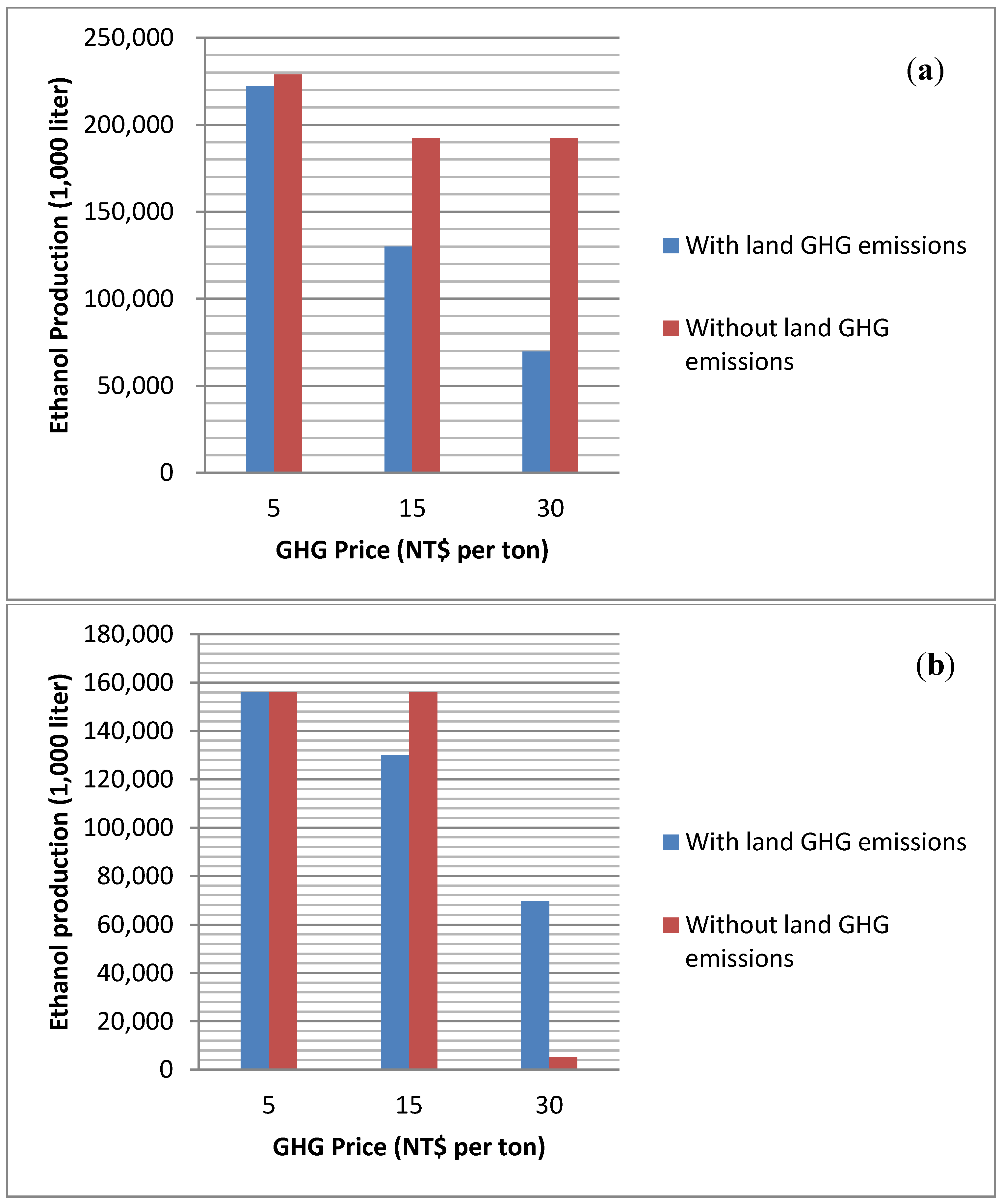
The simulation results indicate that only sweet potato should be used as a feedstock due to its higher production rate, lower cost per ton and harvest frequency (Appendix Table A1). Comparisons between bioenergy production and GHG emission reduction are also provided. Figure 1a,b shows the levels of ethanol production with and without endogenously incorporating land GHG emissions under various GHG prices. We find that when GHG prices increase, ethanol production decreases because ethanol offsets relative less GHG emissions than electricity and under higher GHG prices, ethanol production is replaced by pyrolysis-based electricity. Moreover, when biochar is used as an energy source, ethanol production is higher than when it is used as a soil amendment. This is explained by a combination of high returns to biochar use as a soil amendment, coupled with feedstock competition where more sweet potatoes are used for pyrolysis. However, if GHG price is low, ethanol is the better alternative. However, incorporation of land GHG emissions changes the ethanol production significantly. Ethanol production shrinks dramatically when land emissions are considered, especially for the burning biochar scenarios. This is because emissions from land-use change further reduces the net emissions offset of ethanol production and therefore, ethanol production drops to an even lower level at high GHG prices.

Figure 1. (a) Ethanol production when biochar is burned for energy; (b) Ethanol production when biochar is used as a soil amendment.

Figure 1. (a) Ethanol production when biochar is burned for energy; (b) Ethanol production when biochar is used as a soil amendment.

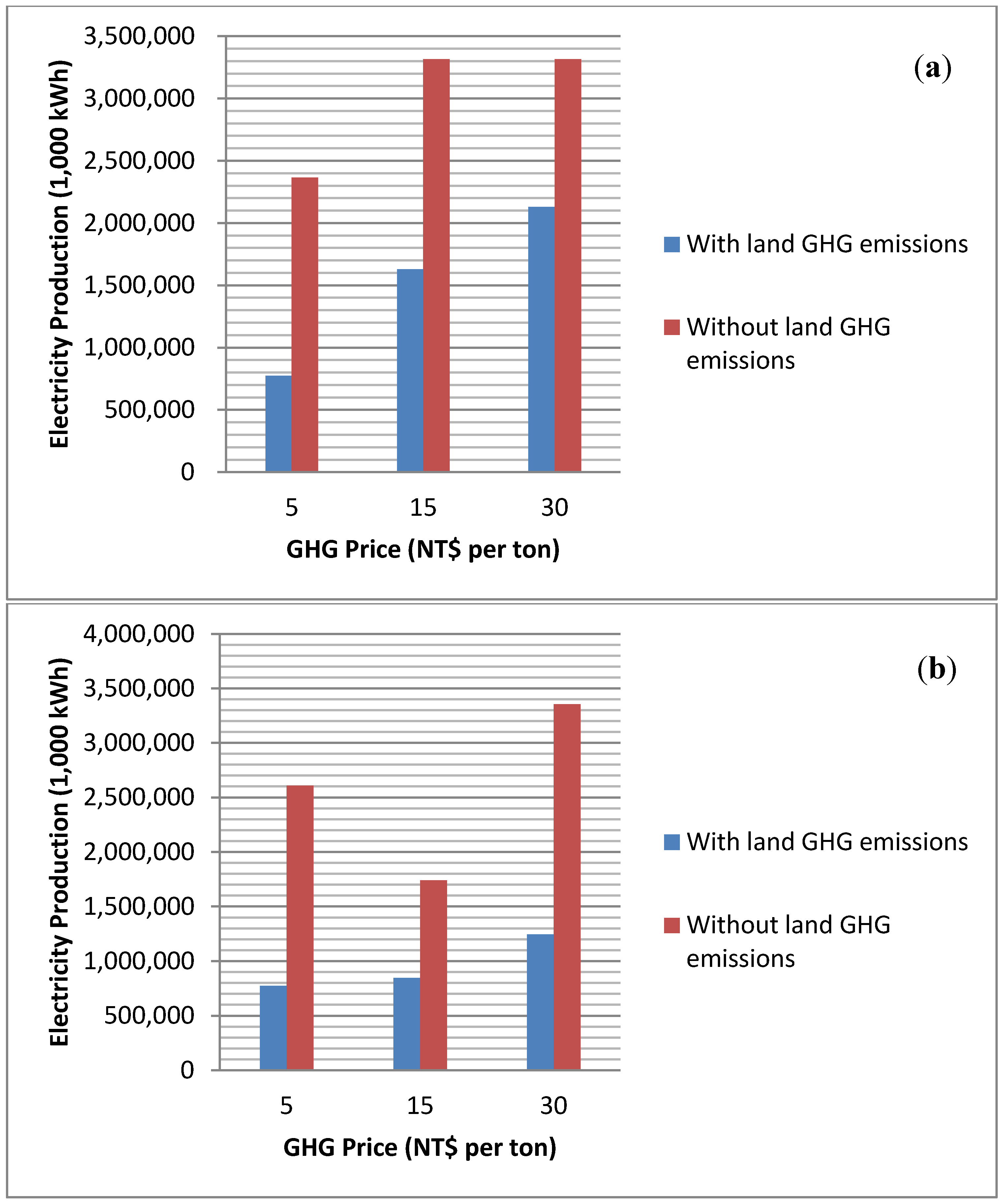
Figure 2a,b shows the levels of electricity production under alternative biochar uses. Here we see that when the GHG price is high, electricity production generally increases. When GHG price is low, producers will adopt fast pyrolysis and generate more electricity. However, when the GHG price becomes higher there is a switch to slow pyrolysis to yield more biochar with an associated reduction in electricity production but an increase in GHG emission offsets. This situation is more obvious when we compare the electricity production under land emissions scenarios. If land emissions are endogenously incorporated, electricity production is generally lower than that under no land emission scenarios. This is due to the higher GHG price has a significant impact on electricity production and hence more sweet potatoes are used in slow pyrolysis to gain better returns. This causes the net electricity production to decrease.

Figure 2. (a) Electricity production when biochar is burned for energy; (b) Electricity production when biochar is used as a soil amendment.

Figure 2. (a) Electricity production when biochar is burned for energy; (b) Electricity production when biochar is used as a soil amendment.

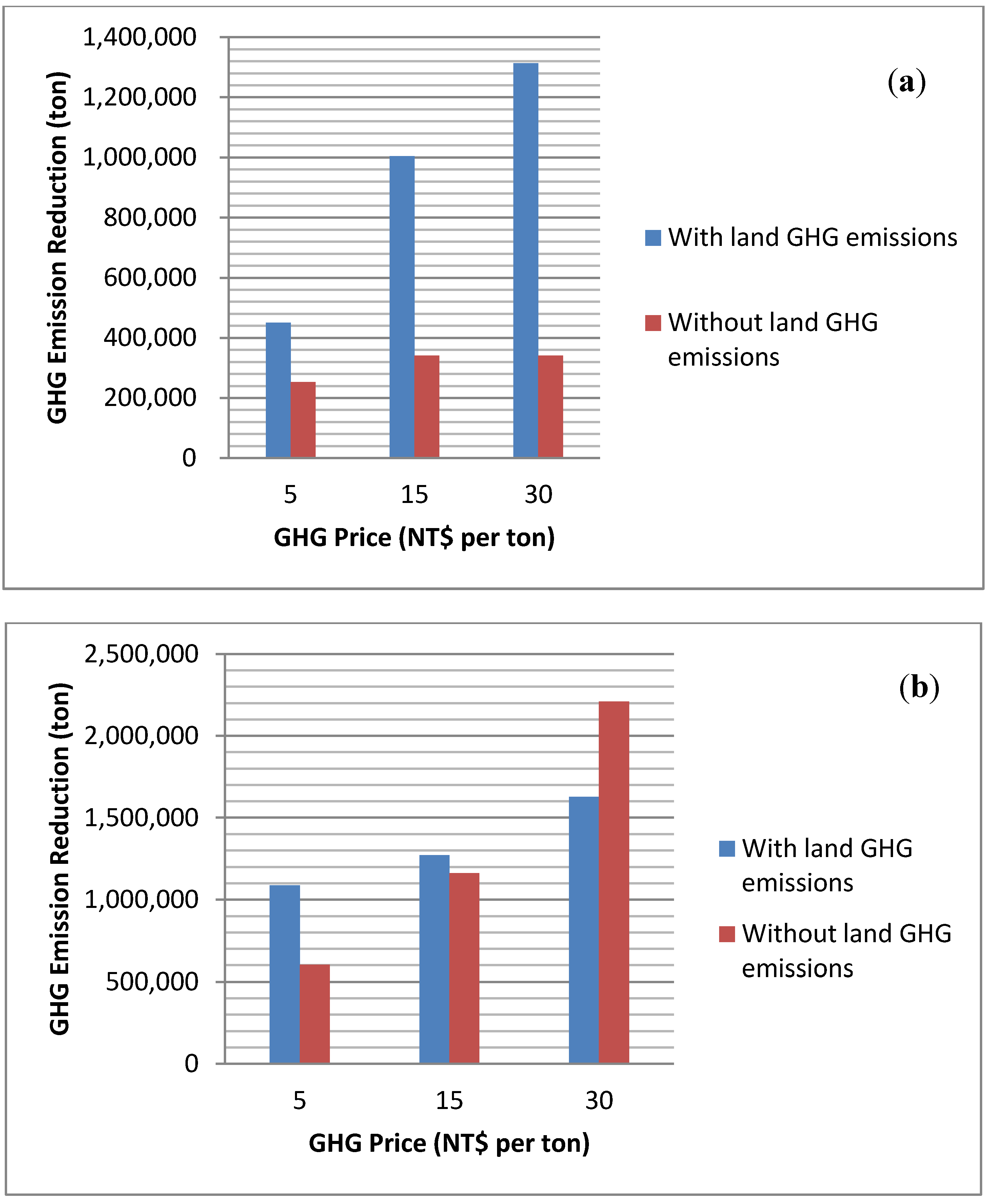
Figure 3a,b indicates the net GHG emissions from bioenergy production. As expected, net GHG emissions offsets increase when the GHG price increases. When land emissions are incorporated and biochar is applied to cropland, the highest net GHG emissions reductions are achieved. This result indicates that there is competition between domestic energy production and climate change mitigation. The result indicates that the largest net GHG emissions reduction occurs when Taiwan’s bioenergy production does not achieve the maximal. Slow pyrolysis and biochar application to crops is the best GHG alternative while fast pyrolysis with the biochar burned for electricity is the best energy alternative. The net GHG emission reduction of burning biochar scenarios when considering land emissions is higher than that in no land emissions scenarios because higher portion of electricity are produced from slow pyrolysis, which yield low electricity but high biochar. However, although slow pyrolysis produces more biochar, land emissions do offset the environmental benefits from using biochar as a soil amendment. Therefore, net emissions offset is lower when land emissions are incorporated.

Figure 3. (a) Net GHG emissions offset when biochar is burned for energy; (b) Net GHG emissions offset when biochar is used as a soil amendment.

Figure 3. (a) Net GHG emissions offset when biochar is burned for energy; (b) Net GHG emissions offset when biochar is used as a soil amendment.

The study also shows that when multiple bioenergy techniques such as ethanol, conventional electricity and pyrolysis-based electricity are competing with each other, conventional electricity is not competitive. The results also indicate that when land GHG emissions are incorporated, ethanol production decreases across all scenarios. Throughout all scenarios, simulation result can be interpreted as:

(1)

When land GHG emissions are endogenously considered, electricity and ethanol production will have a significant shrink, compared to the no land emissions scenarios.

(2)

When biochar is used as an energy source, more sweet potatoes are used in fast pyrolysis and lead to a larger reduction on ethanol production.

(3)

Slow pyrolysis dominates fast pyrolysis, ethanol and conventional electricity at high GHG price. Fast pyrolysis dominates all other alternatives at low GHG price.

(4)

Net GHG emission offset will increase in burning biochar scenarios but decrease in hauling biochar scenarios. The maximum amount of GHG emissions reduction from Taiwanese bioenergy production is lower when land emissions are endogenously considered into the production process.

(5)

If land GHG emissions are not considered, simulation result for ethanol and electricity production and GHG emissions reduction will be too optimistic.

6. Conclusions

This study examined the trade-off relationship between Taiwanese bioenergy production and associated GHG emissions when ethanol, conventional bioelectricity and pyrolysis-based bioelectricity can be produced. The results show that when biochar is for electricity that, pyrolysis can provide up to 3.8 billion kWh or about 1.73% of Taiwan’s annual electricity demand while offsetting up to 2.2 million tons of GHG emissions (or 1.58% of Taiwan’s annual GHG emissions).

We find that ethanol will not be competitive when land based emissions are considered under high GHG prices because of its low GHG offset levels. However, when ethanol price is higher than NT$40 per liter and GHG price is lower than NT$15 per ton, ethanol production is desirable and provides a substantial amount of ethanol for blended gasoline. Based on the simulation results, there are tradeoffs between energy production and GHG offsets and between electricity and ethanol production.

Those crafting Taiwan’s bioenergy strategy may well want to consider these tradeoffs. Larger amounts of imported energy can be replaced with production of ethanol and fast pyrolysis based electricity but larger GHG emissions reductions occur with slow pyrolysis based electricity and land application of biochar. The result indicates that when land use emissions are endogenously incorporated, the best technique for climate change mitigation is slow pyrolysis and both ethanol and pyrolysis based electricity will decrease significantly. However, fast pyrolysis would still be a better technique for the concern of energy security and most of ethanol and conventional bioelectricity would be driven out.

This study has limitations. The findings are a reflection of the assumptions used such as feedstock yields, energy recovery rates, pyrolysis yields and land emission rates. The accuracy of such assumptions could be improved. Also we also ignore the differences of weather and soil between counties that may actually lead to different crop yields and biochar application effects. These limitations can be addressed once related experimental data is available.

References

- Intergovernmental Panel on Climate Change (IPCC). Guidelines for National Greenhouse Gas Inventories; Cambridge University Press: Cambridge, UK, 2007. [Google Scholar]
- Kung, C.C.; McCarl, B.A.; Cao, X.Y.; Xie, H.L. Bioenergy prospects in Taiwan using set-aside land—An economic evaluation. China Agr. Econ. Rev. 2013, 4, 489–511. [Google Scholar]
- Liu, H.; Zhao, P.; Lu, P.; Wang, Y.S.; Lin, Y.B.; Rao, X.Q. Greenhouse gases fluxes from soils of different land-use types in a hilly area of south China. Agr. Ecosyst. Environ. 2007, 124, 125–135. [Google Scholar]
- Grover, S.P.P.; Liverley, S.J.; Hutley, I.B.; Jamall, H.; Fest, B.; Beringer, J.; Butterbach-Bahl, K.; Arndt, S.K. Land use change and the impact on greenhouse gas exchange in north Australian savanna soils. Biogeosciences 2012, 9, 423–437. [Google Scholar] [CrossRef]
- Ringer, M.; Putsche, V.; Scahill, J. Large-scale pyrolysis oil production: A technology assessment and economic analysis. Environ. Sci. 2006, 17, 21–33. [Google Scholar]
- Wright, M.M.; Brown, R.C.; Boateng, A.A. Distributed processing of biomass to biooil for subsequent production of Fischer-tropsch liquids. Biofuels Bioprocessing Biorefining 2008, 2, 229–238. [Google Scholar] [CrossRef]
- Lehmann, J. A handful of carbon. Nature 2007, 447, 143–144. [Google Scholar] [CrossRef]
- Lehmann, J.; Gaunt, J.; Rondon, M. Biochar sequestration in terrestrial ecosystems—A review. Mitigation Adaption Strategy Glob. Change 2006, 11, 403–427. [Google Scholar]
- Kung, C.C.; McCarl, B.A.; Cao, X.Y. Economics of pyrolysis-based energy production and biochar utilization: A case study in Taiwan. Energ. Policy 2013, 60, 317–323. [Google Scholar] [CrossRef]
- Deluca, T.H.; MacKenzie, M.D.; Gundale, M.J. Biochar Effects on Soil Nutrient Transformations. In Biochar for Environmental Management; Lehmann, J., Joseph, S., Eds.; Earthscan Publisher: London, UK, 2009; pp. 137–182. [Google Scholar]
- McCarl, B.A.; Peacocke, C.; Chrisman, R.; Kung, C.C.; Sands, R.D. Economics of Biochar Production, Utilization, and GHG Offsets. In Biochar for Environmental Management: Science and Technology; Lehmann, J., Joseph, S., Eds.; Earthscan Publisher: London, UK, 2009; pp. 341–357. [Google Scholar]
- Glaser, B.; Lehmann, J.; Zech, W. Ameliorating physical and chemical properties of highly weathered soils in the tropics with charcoal—A review. Biol. Fert. Soils 2002, 35, 219–230. [Google Scholar] [CrossRef]
- Steiner, T.; Mosenthin, R.; Zimmermann, B.; Greiner, R.; Roth, S. Distribution of phytase activity, total phosphorus and phytate phosphorus in legume seeds, cereals and cereal products as influenced by harvest year and cultivar. Anim. Feed Sci. Tech. 2007, 133, 320–334. [Google Scholar] [CrossRef]
- Lehmann, J.; Silva, J.P.; Steiner, C.; Nehls, T.; Zech, W.; Glaser, B. Nutrient availability and leaching in an archaeological anthrosol and a ferralsol of the central Amazon basin: Fertilizer, manure and charcoal amendments. Plant Soil 2003, 249, 343–357. [Google Scholar] [CrossRef]
- Chan, K.Y.; Zwieten, L.; Meszaros, I.; Downie, A.; Joseph, S. Agronomic values of green waste biochar as a soil amendment. Aust. J. Soil Res. 2007, 45, 629–634. [Google Scholar] [CrossRef]
- Free, H.F.; McGill, C.R.; Rowarth, J.S.; Hedley, M.J. The effect of biochars on maize germination. N. Z. J. Agr. Res. 2010, 53, 1–4. [Google Scholar] [CrossRef]
- Iswaran, V.; Jauhri, K.S.; Sen, A. Effect of charcoal, coal and peat on the yield of moong, soybean and pea. Soil Biol. Biochem. 1980, 12, 191–192. [Google Scholar] [CrossRef]
- Kishimoto, S.; Sugiura, G. Charcoal as a soil conditioner. Int. Ach. Future 1985, 5, 12–23. [Google Scholar]
- Chidumayo, E.N. Phenology and nutrition of miombo woodland trees in Zambia. Trees 1994, 9, 67–72. [Google Scholar] [CrossRef]
- Oguntunde, P.G.; Abiodun, B.J.; Ajayi, A.E.; Giesen, N. Effects of charcoal production on soil physical properties in Ghana. J. Plant Nutr. Soil Sci. 2004, 171, 591–596. [Google Scholar]
- Nehls, T. Fertility improvement of terra firme oxisol in central Amazonia by charcoal applications. Environ. Sci. 2002, 14, 21–45. [Google Scholar]
- Wang, M. Well-to-wheelsEnergy and Greenhouse Gas Emission Results of Fuel Ethanol; Argonne National Laboratory: Lemont, IL, USA, 2007.
- Schaufler, G.; Kitzler, B.; Schindlbacher, A.; Skiba, U.; Sutton, M.A.; Zechmeister-Boltenstern, S. Greenhouse gas emissions from european soils under different land use: Effects of soil moisture and temperature. Eur. J. Soil Sci. 2010, 61, 683–696. [Google Scholar] [CrossRef]
- Baldos, U.L.C. A Sensitivity Analysis of the Lifecycle and Global Land Use Change Greenhouse Gas Emissions of U.S. Corn Ethanol Fuel. Master Thesis, Purdue University, West Lafayette, IN, USA, 2009. [Google Scholar]
- Baggs, E.M.; Stevenson, M.; Pihlatie, M.; Regar, A.; Cook, H.; Cadisch, G. Nitrous oxide emissions following application of residues and fertilizer under zero and conventional tillage. Plant Soil 2003, 254, 361–370. [Google Scholar] [CrossRef]
- Farquharson, J.; Baldock, J. Concepts in modeling n2o emissions from land use. Plant Soil 2008, 309, 17–167. [Google Scholar]
- Wang, M.; Saricks, C.; Santini, D. Effects of Fuel Ethanol Use on Fuel-cycle Energy and Greenhouse Gas Emissions; Center for Transportation Research, Argonne National Laboratory: Argonne, IL, USA, 1999.
- Searchinger, T.; Heimlich, R.; Houghton, R.A.; Dong, F.; Elobeid, A.; Fabiosa, J.; Tokgoz, S.; Hayes, D.; Yu, T.-H. Use of U.S. croplands for biofuels increases greenhouse gases through emissions from land-use change. Science 2008, 319, 1238–1240. [Google Scholar] [CrossRef]
- Fargione, J.; Hill, J.; Tilman, D.; Polasky, S.; Hawthorne, P. Land clearing and the biofuel carbon debt. Science 2008, 319, 1235–1238. [Google Scholar] [CrossRef]
- Hill, J.; Polaskya, S.; Nelson, E.; Tilman, D.; Huo, H.; Ludwig, L.; Neumann, J.; Zheng, H.; Bonta, D. Climate change and health costs of air emissions from biofuels and gasoline. Pro. Nat. Acad. Sci. USA 2008, 106, 2077–2082. [Google Scholar]
- Kim, H.; Kim, S.; Dale, B.E. Biofuels, land use change, and greenhouse gas emissions: Some unexplored variable. Environ. Sci. Technol. 2009, 43, 961–967. [Google Scholar] [CrossRef]
- Samuelson, P.A. Spatial price equilibrium and linear programming. Amer. Econ. Rev. 1950, 42, 283–303. [Google Scholar]
- Chen, C.C.; Chang, C.C. The impact of weather on crop yield distribution in Taiwan: Some new evidence from panel data models and implications for crop insurance. J. Agr. Econ. 2005, 33, 503–511. [Google Scholar] [CrossRef]
- McCarl, B.A.; Spreen, T.H. Price endogenous mathematical programming as a tool for sector analysis. Amer. J. Agr. Econ. 1980, 62, 87–102. [Google Scholar] [CrossRef]
- Chang, C.C.; McCarl, B.A.; Mjelde, J.; Richardson, J.W. Sectoral implications of farm program modifications. Amer. J. Agr. Econ. 1992, 74, 38–49. [Google Scholar] [CrossRef]
- Coble, K.H.; Chang, C.C.; McCarl, B.A.; Eddleman, B.R. Assessing economic implications of new technology: The case of cornstarch-based biodegradable plastics. Rev. Agric. Econ. 1992, 14, 33–43. [Google Scholar] [CrossRef]
- Chang, C.C. The potential impacts of climate change on Taiwan’s agriculture. Agr. Econ. 2002, 27, 51–64. [Google Scholar] [CrossRef]
- McCarl, B.A.; Schneider, U.A. Greenhouse gas mitigation in us agriculture and forestry. Science 2001, 294, 2481–2482. [Google Scholar]
- Aylott, M.J.; Casella, E.; Farrall, K.; Taylor, G. Estimating the supply of biomass from short-rotation coppice in England. Biofuels 2009, 12, 719–727. [Google Scholar]
- McCarl, B.A.; Adams, D.M.; Alig, R.J.; Chmelik, J.T. Analysis of biomass fueled electrical power plants: Implications in the agricultural and forestry sectors. Ann. Oper. Res. 2000, 94, 37–55. [Google Scholar] [CrossRef]
- Beach, R.H.; McCarl, B.A. U.S. Agricultural and Forestry Impacts of the Energy Independence and Security Act: FASOM Results and Model Description; Office of Transportation and Air Quality, U.S. Environmental Protection Agency: Washington, DC, USA, 2010.
- Beach, R.H.; Adams, D.M.; Alig, R.J.; Baker, J.S.; Latta, G.S.; McCarl, B.A.; Murray, B.C.; Rose, S.K.; White, E. Model Documentation for the Forest and Agricultural Sector Optimization Model with Greenhouse Gases (FASOMGHG); Climate Change Division, U.S. Environmental Protection Agency: Washington, DC, USA, 2010.
- Weber, J.A.; Johannes, K. Biodiesel market opportunities and potential barriers. Amer. Soc. Agr. Eng. 1996, 25, 366–375. [Google Scholar]
- McCarl, B.A. Food, biofuel, global agriculture, and environment: Discussion. Rev. Agric. Econ. 2008, 30, 530–532. [Google Scholar] [CrossRef]
- He, F.; Yi, W.; Zha, J. Measurement of the heat of smoldering combustion in straws and stalks by means of simultaneous thermal analysis. Biomass Bioenerg. 2009, 33, 130–136. [Google Scholar] [CrossRef]
- Bridgwater, A.V.; Peacocke, G.V.C. Fast pyrolysis processes for biomass. Renew. Sustain. Energy Rev. 2002, 4, 1–73. [Google Scholar] [CrossRef]
- Tola, V.; Cau, G. Process analysis and performance evaluation of updraft coal gasifier. Clean Technol. 2007, 28, 15–31. [Google Scholar]
- Gaunt, J.L.; Lehmann, J. Energy balance and emissions associated with biochar sequestration and pyrolysis bioenergy production. Environ. Sci. Technol. 2008, 42, 4152–4158. [Google Scholar] [CrossRef]
- Qin, Z.; Zhuang, Q.; Zhu, X. Carbon and nitrogen dynamics in bioenergy ecosystems: 2. Potential greenhouse gas emissions and global warming intensity in the conterminous United States. Bioenergy 2013. [Google Scholar] [CrossRef]
- Snyder, C.S.; Bruulsema, T.W.; Jensen, T.L.; Fixen, P.E. Review of greenhouse gas emissions from crop production systems and fertilizer management effects. Agr. Ecosyst. Environ. 2009, 133, 247–266. [Google Scholar] [CrossRef]
Appendix
Table A1.
Simulation results of bioenergy production and GHG emissions offset for with and without endogenous land GHG emissions.