A GIS Based Approach for Assessing the Association between Air Pollution and Asthma in New York State, USA


Abstract
:1. Introduction
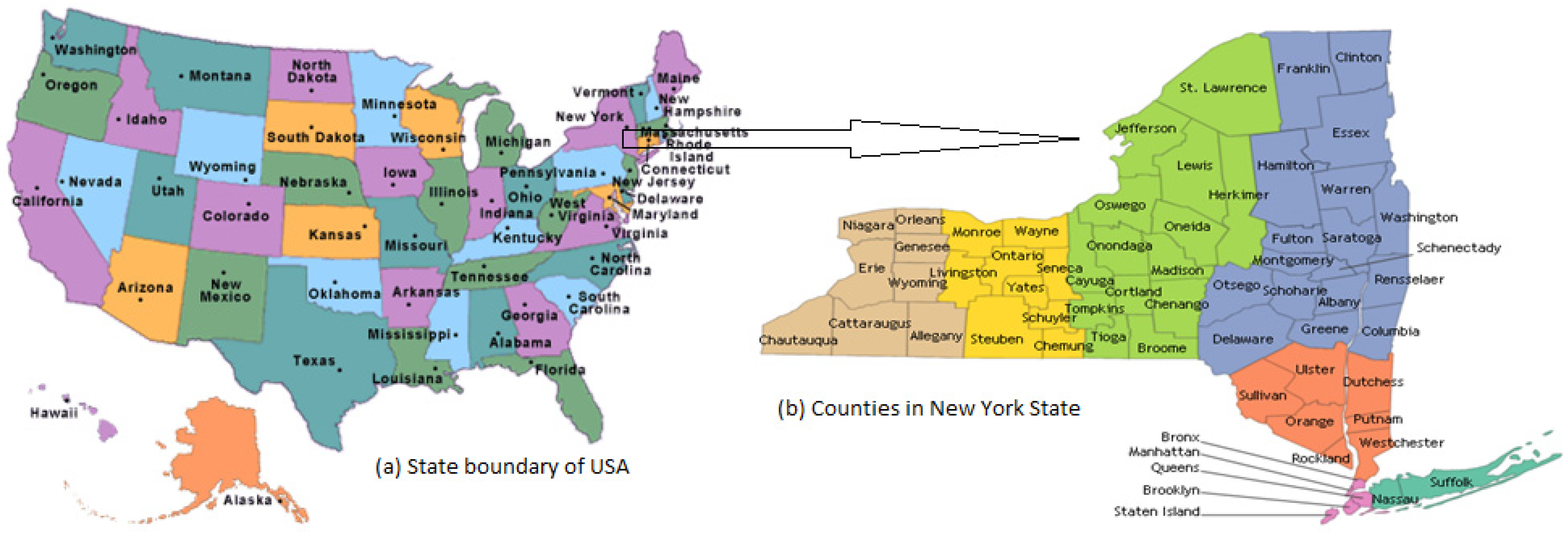
2. Study Area

3. Materials and Methods
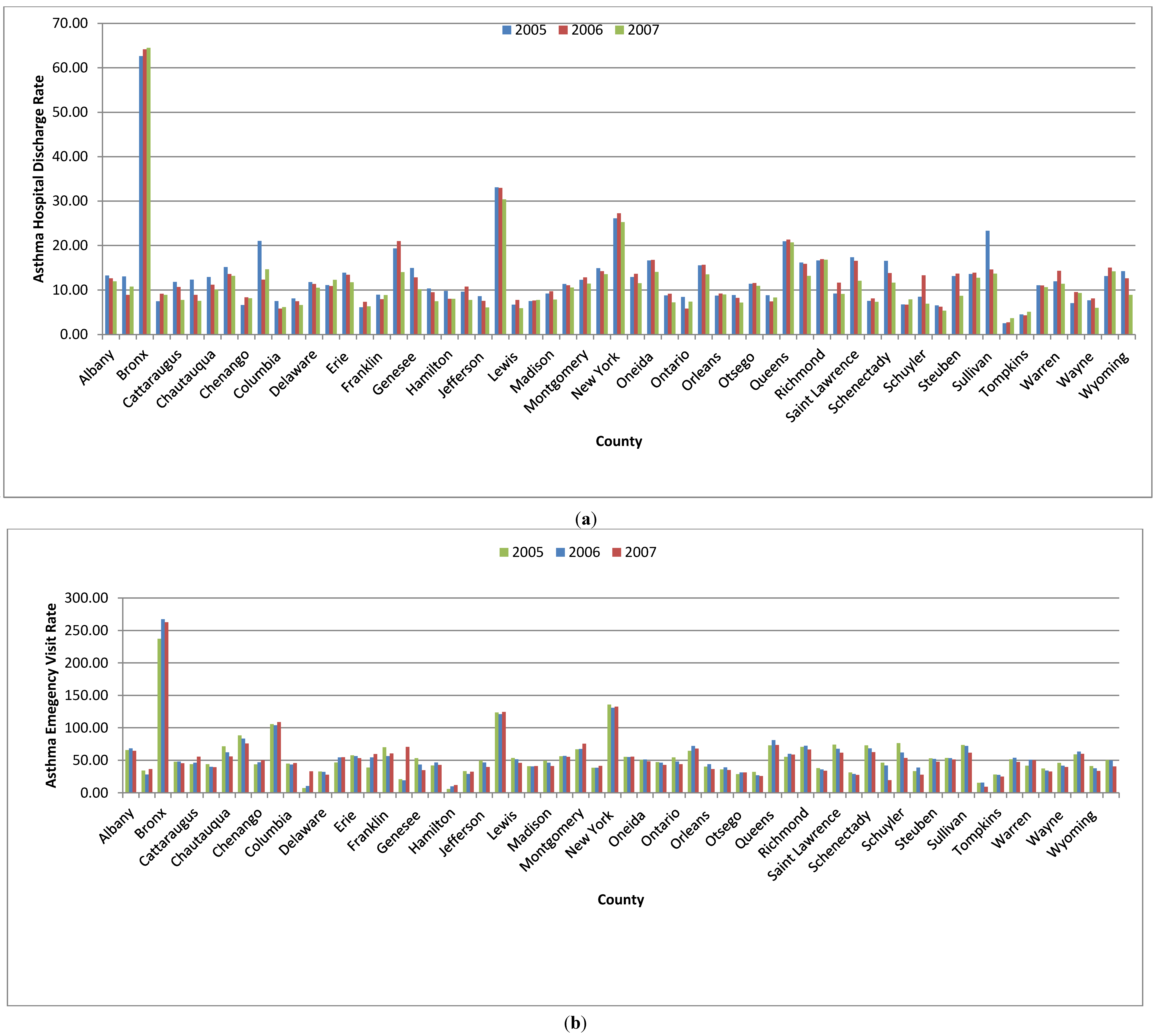
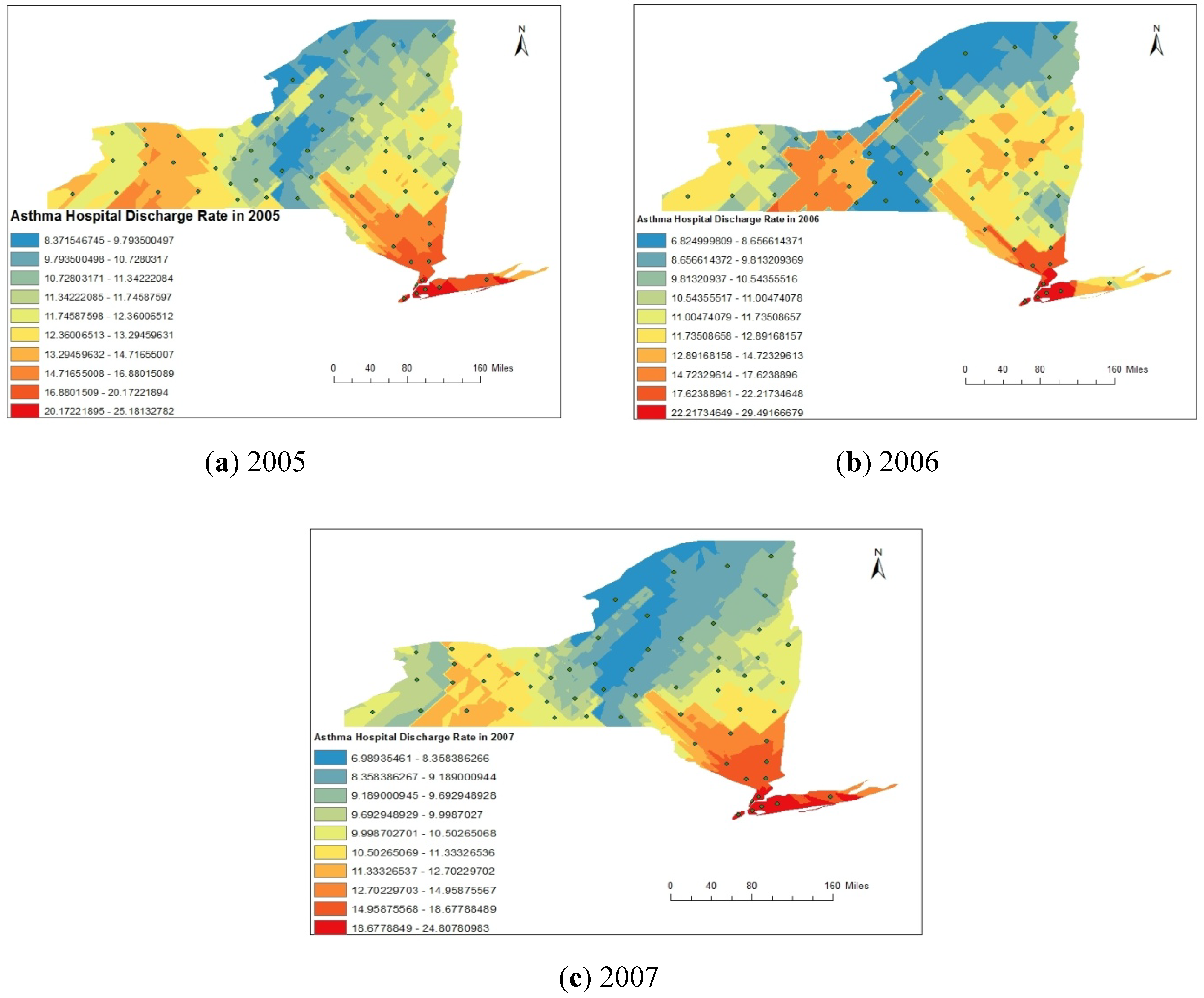
3.1. Hospital Admission Data
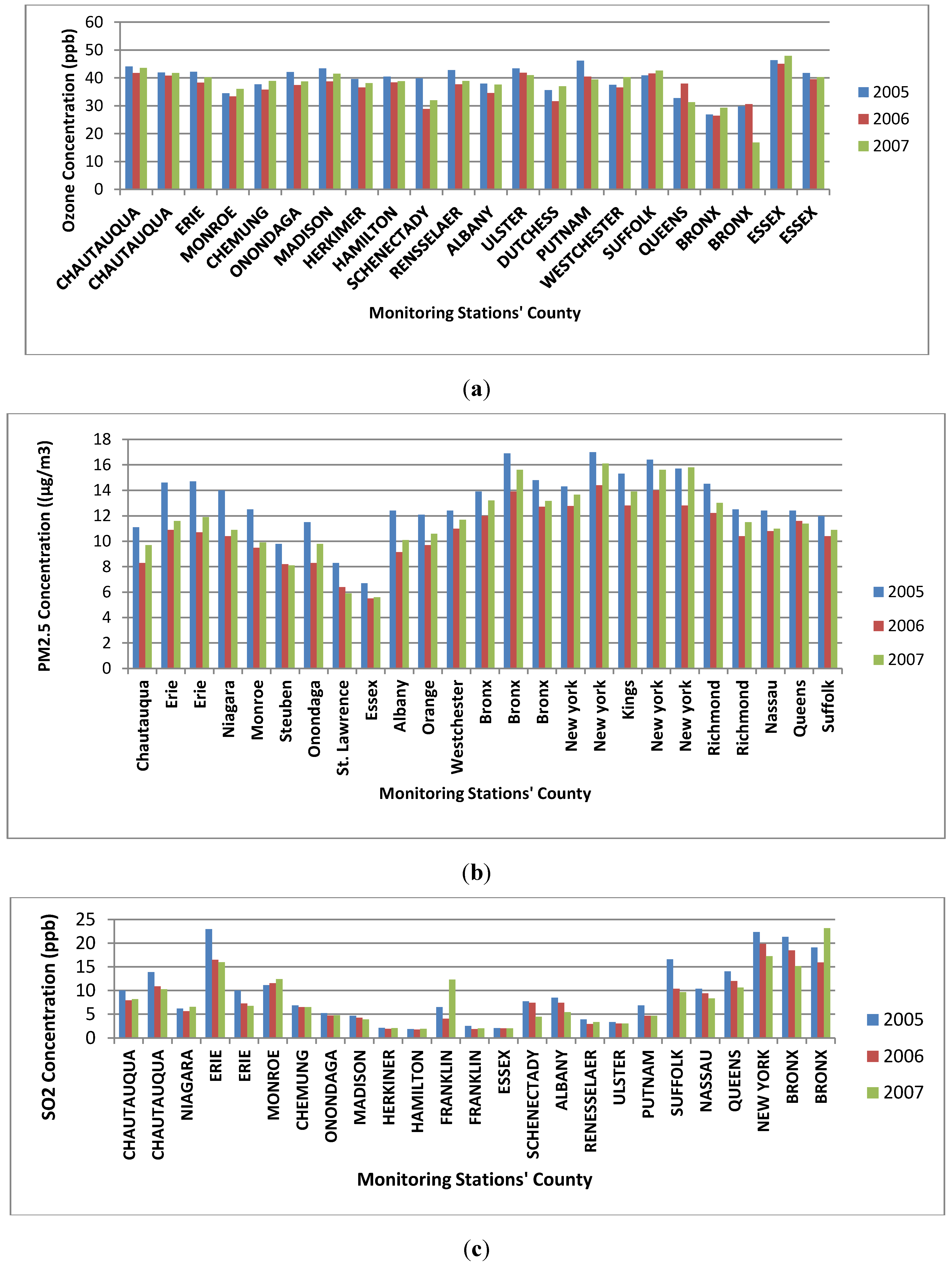
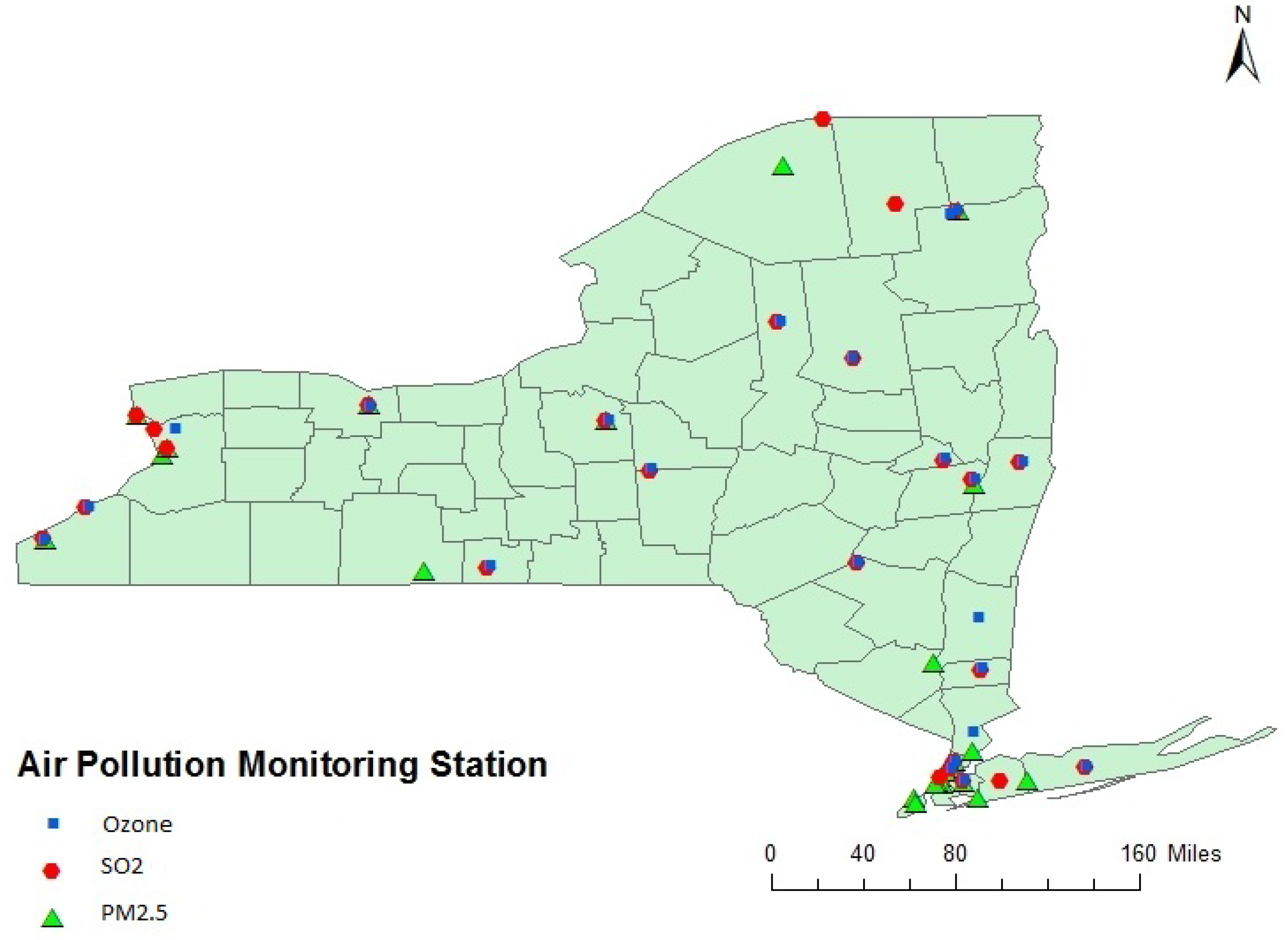
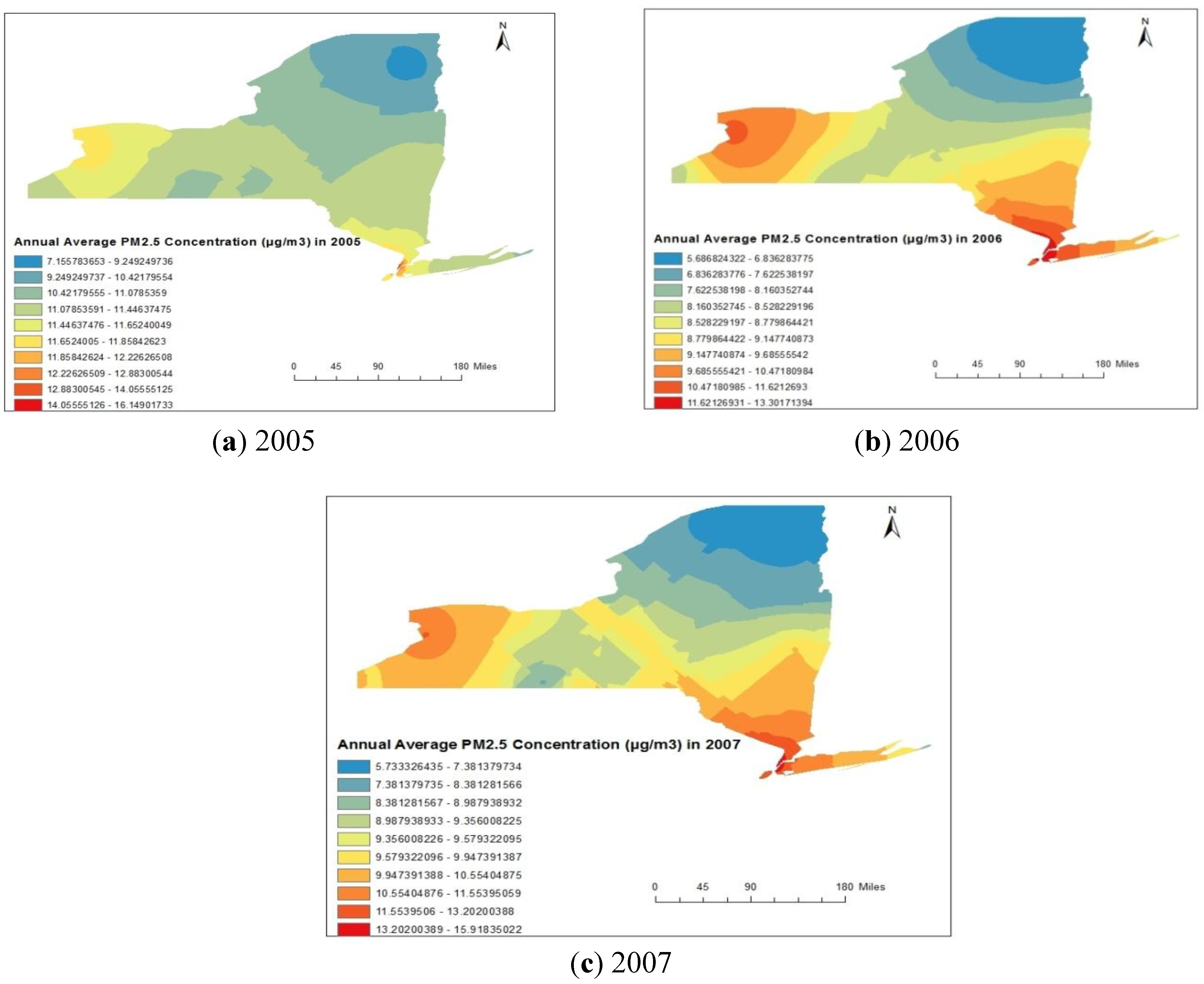
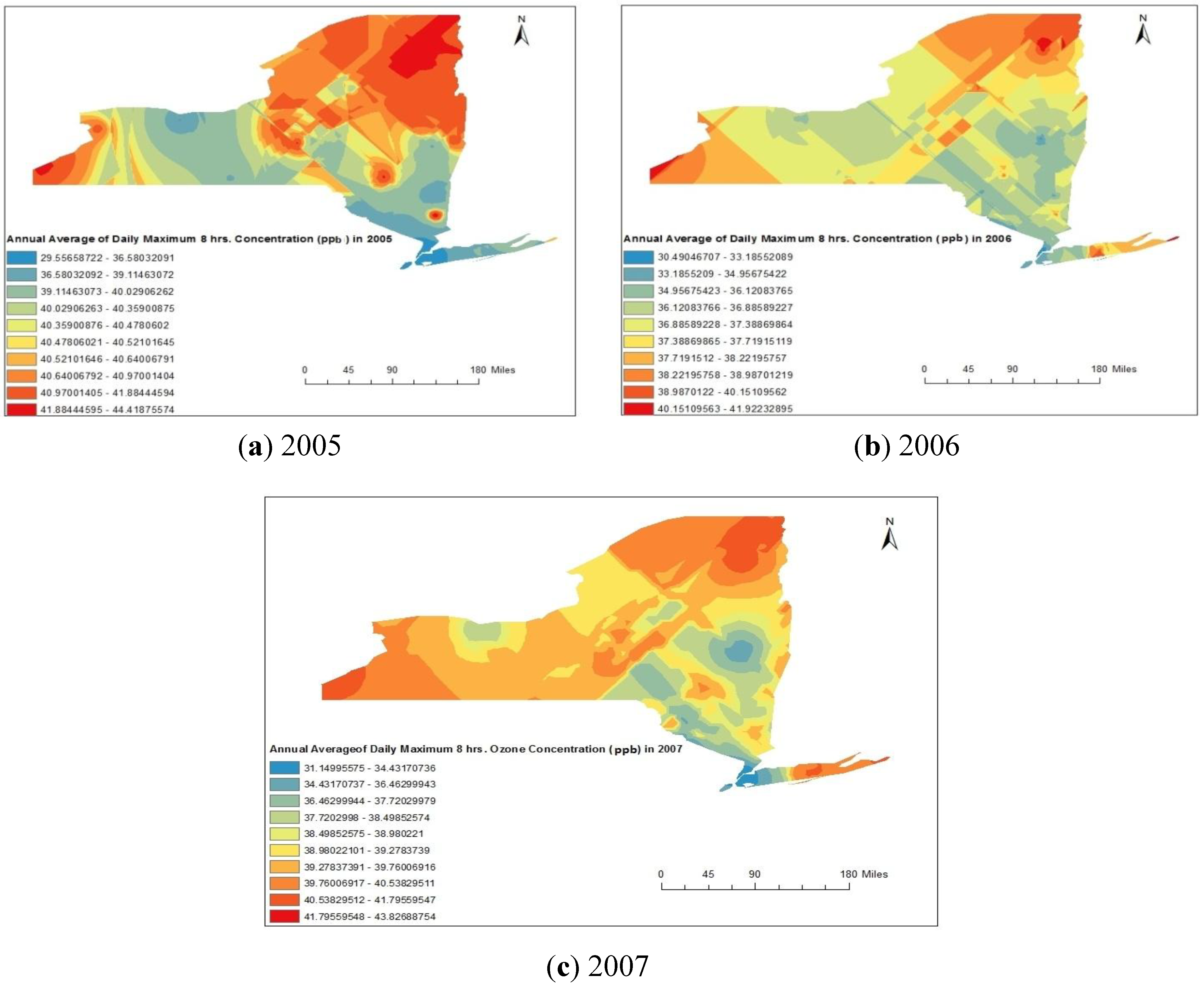
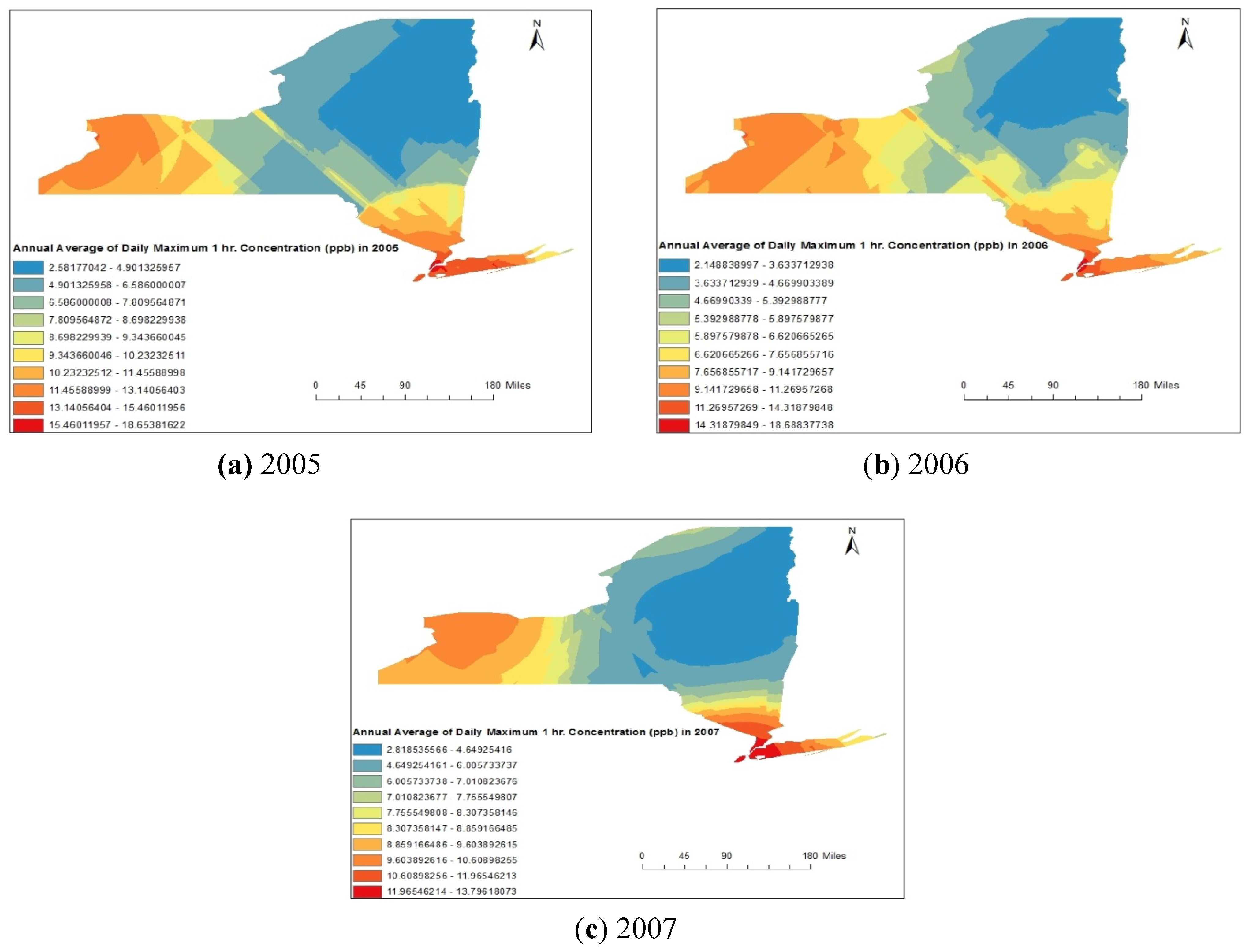
3.2. Air Pollution Data

| Items | Minimum | Maximum | Mean | Standard Deviation |
|---|---|---|---|---|
| 2005 | ||||
| Asthma Rate | 37.77 | 94.05 | 53.04 | 8.39 |
| Ozone | 29.56 | 44.48 | 40.21 | 1.17 |
| PM2.5 | 7.15 | 16.15 | 11.39 | 1.15 |
| SO2 | 2.58 | 18.65 | 8.46 | 2.88 |
| 2006 | ||||
| Asthma Rate | 37.34 | 98.30 | 52.46 | 9.77 |
| Ozone | 30.49 | 41.92 | 37.42 | 1.21 |
| PM2.5 | 5.68 | 13.30 | 8.73 | 1.05 |
| SO2 | 2.14 | 18.69 | 6.91 | 2.31 |
| 2007 | ||||
| Asthma Rate | 36.56 | 94.87 | 50.96 | 10.43 |
| Ozone | 31.75 | 42.69 | 39.08 | 1.76 |
| PM2.5 | 5.73 | 15.91 | 9.49 | 1.08 |
| SO2 | 2.81 | 13.79 | 7.18 | 2.38 |
4. Results and Discussion
4.1. Spatial Analysis Using GIS

| Parameter | Fitted Model | Nugget | Partial Sill | Lag Size (in degree) | Range(in degree) | MSE | RMSSE |
|---|---|---|---|---|---|---|---|
| Ozone | |||||||
| 2005 | Stable | 0 | 29.78 | 0.32 | 3.79 | −0.03 | 0.80 |
| 2006 | Stable | 0 | 30.11 | 0.08 | 0.66 | −0.006 | 0.83 |
| 2007 | Stable | 9.66 | 16.72 | 0.08 | 0.67 | 0.001 | 0.77 |
| PM2.5 | |||||||
| 2005 | Stable | 0.85 | 6.52 | 0.30 | 2.46 | 0.09 | 0.76 |
| 2006 | Stable | 0.72 | 7.68 | 0.34 | 2.70 | 0.07 | 0.68 |
| 2007 | Stable | 0.01 | 8.13 | 0.30 | 2.41 | 0.08 | 0.69 |
| SO2 | |||||||
| 2005 | Stable | 0 | 31.79 | 0.17 | 1.38 | 0.00 | 0.83 |
| 2006 | Stable | 0 | 24.14 | 0.17 | 1.42 | 0.02 | 0.77 |
| 2007 | Stable | 21.49 | 13.22 | 0.26 | 2.14 | −0.01 | 0.85 |

4.2. Statistical Analyses
4.2.1. Map Correlation Analysis
| 2005 | |||||
|---|---|---|---|---|---|
| AEVR | ADR | O3 | PM2.5 | SO2 | |
| AEVR * | 1.00 | ||||
| ADR ** | 0.84 | 1.00 | |||
| O3 | −0.54 | −0.55 | 1.00 | ||
| PM2.5 | 0.29 | 0.39 | −0.56 | 1.00 | 0.82 |
| SO2 | 0.46 | 0.52 | −0.59 | 0.82 | 1.00 |
| 2006 | |||||
| AEVR | ADR | O3 | PM2.5 | SO2 | |
| AEVR | 1.00 | ||||
| ADR | 0.54 | 1.00 | |||
| O3 | −0.25 | −0.25 | 1.00 | ||
| PM2.5 | 0.39 | 0.46 | −0.41 | 1.00 | |
| SO2 | 0.31 | 0.38 | −0.30 | 0.86 | 1.00 |
| 2007 | |||||
| AEVR | ADR | O3 | PM2.5 | SO2 | |
| AEVR | 1.00 | ||||
| ADR | 0.86 | 1.00 | |||
| O3 | −0.42 | −0.49 | 1.00 | ||
| PM2.5 | 0.25 | 0.53 | −0.48 | 1.00 | |
| SO2 | 0.13 | 0.41 | −0.33 | 0.73 | 1.00 |
4.2.2. Point Correlation Analysis
| County Name | ADR | AEVR | Ozone Concentration (ppb) | PM2.5 Concentration (µg/m3) | SO2 Concentration (ppb) | ||||||||||
|---|---|---|---|---|---|---|---|---|---|---|---|---|---|---|---|
| 2005 | 2006 | 2007 | 2005 | 2006 | 2007 | 2005 | 2006 | 2007 | 2005 | 2006 | 2007 | 2005 | 2006 | 2007 | |
| Clinton | 21.04 | 12.36 | 14.66 | 105.55 | 103.94 | 108.77 | 42.38 | 39.91 | 41.97 | 8.45 | 6.04 | 6.94 | 3.20 | 2.40 | 4.18 |
| Franklin | 8.97 | 7.96 | 8.88 | 69.84 | 56.49 | 60.45 | 41.54 | 38.86 | 40.49 | 8.63 | 6.09 | 7.04 | 3.67 | 2.82 | 4.88 |
| Essex | 6.10 | 7.34 | 6.35 | 38.66 | 54.19 | 59.69 | 42.02 | 38.08 | 39.41 | 8.56 | 6.21 | 7.13 | 3.66 | 3.05 | 3.21 |
| Hamilton | 9.82 | 8.02 | 8.05 | 5.89 | 10.03 | 12.07 | 41.04 | 37.67 | 39.62 | 9.97 | 7.24 | 8.14 | 4.03 | 3.05 | 3.06 |
| Herkimer | 9.64 | 10.78 | 7.77 | 33.44 | 29.05 | 32.48 | 40.87 | 36.37 | 38.18 | 10.50 | 7.75 | 8.70 | 4.00 | 3.40 | 3.25 |
| Washington | 7.04 | 9.56 | 9.36 | 37.14 | 34.25 | 32.83 | 41.15 | 38.31 | 40.23 | 10.46 | 8.06 | 8.72 | 4.16 | 3.64 | 3.68 |
| Warren | 11.96 | 14.34 | 11.41 | 41.56 | 50.95 | 50.05 | 41.28 | 37.37 | 39.31 | 9.80 | 7.40 | 8.07 | 4.01 | 3.45 | 3.14 |
| Saratoga | 17.38 | 16.58 | 12.10 | 74.10 | 67.59 | 61.48 | 41.12 | 36.43 | 39.01 | 10.96 | 8.31 | 9.13 | 4.28 | 4.07 | 3.57 |
| Fulton | 19.35 | 20.97 | 10.06 | 20.98 | 19.16 | 70.46 | 40.67 | 36.06 | 38.10 | 10.76 | 8.16 | 8.98 | 4.50 | 3.66 | 3.22 |
| Montgomery | 12.32 | 12.87 | 11.45 | 66.86 | 67.37 | 75.51 | 40.53 | 35.97 | 38.09 | 10.99 | 8.43 | 9.17 | 4.83 | 4.15 | 3.66 |
| Rensselaer | 16.21 | 15.89 | 13.21 | 55.22 | 59.82 | 58.71 | 40.64 | 36.38 | 38.81 | 11.63 | 8.91 | 9.66 | 6.32 | 4.90 | 4.67 |
| Schenectady | 7.56 | 8.11 | 7.37 | 31.41 | 29.07 | 27.53 | 40.30 | 35.67 | 39.10 | 11.35 | 8.69 | 9.41 | 5.02 | 4.99 | 4.03 |
| Otsego | 11.42 | 11.58 | 10.97 | 28.70 | 31.57 | 31.31 | 40.13 | 36.36 | 35.98 | 11.00 | 8.57 | 9.28 | 7.37 | 5.92 | 4.08 |
| Schoharie | 16.58 | 13.84 | 11.69 | 72.84 | 68.13 | 62.52 | 40.61 | 36.10 | 38.10 | 11.25 | 8.76 | 9.42 | 4.89 | 4.22 | 4.14 |
| Albany | 13.28 | 12.63 | 11.95 | 65.72 | 68.16 | 64.60 | 39.90 | 35.72 | 38.23 | 11.70 | 8.98 | 9.69 | 6.91 | 6.04 | 4.39 |
| Delaware | 11.78 | 11.39 | 10.53 | 32.87 | 32.32 | 27.86 | 40.14 | 35.54 | 34.66 | 11.19 | 8.91 | 9.50 | 7.58 | 6.15 | 5.09 |
| Columbia | 7.53 | 5.83 | 6.15 | 44.89 | 43.20 | 45.72 | 39.36 | 36.12 | 38.20 | 11.82 | 9.20 | 10.01 | 7.60 | 6.24 | 5.39 |
| Greene | 10.38 | 9.49 | 7.47 | 41.92 | 46.45 | 42.80 | 40.22 | 36.39 | 38.22 | 11.65 | 9.11 | 9.81 | 6.82 | 5.60 | 5.11 |
| Ulster | 11.07 | 11.05 | 10.67 | 51.52 | 53.76 | 47.31 | 39.92 | 36.78 | 36.60 | 11.83 | 9.40 | 10.19 | 9.71 | 7.09 | 6.81 |
| Dutchess | 11.11 | 10.89 | 12.33 | 46.41 | 54.32 | 54.69 | 37.66 | 35.17 | 39.37 | 11.95 | 9.47 | 10.37 | 10.05 | 7.50 | 7.79 |
| Sullivan | 23.31 | 14.63 | 13.72 | 73.59 | 72.12 | 61.55 | 39.19 | 35.33 | 36.09 | 11.96 | 9.58 | 10.35 | 10.63 | 8.21 | 7.27 |
| Orange | 15.55 | 15.70 | 13.54 | 64.58 | 72.01 | 68.04 | 38.90 | 36.30 | 35.64 | 12.42 | 10.47 | 10.96 | 11.23 | 8.73 | 9.74 |
| Putnam | 8.84 | 7.45 | 8.35 | 32.44 | 21.17 | 25.94 | 41.49 | 37.18 | 36.30 | 12.24 | 10.01 | 10.84 | 10.79 | 7.09 | 9.52 |
| Westchester | 13.15 | 15.04 | 14.23 | 59.00 | 63.31 | 59.89 | 38.22 | 36.12 | 35.29 | 12.73 | 10.74 | 11.50 | 12.26 | 9.70 | 10.97 |
| Rockland | 9.21 | 11.69 | 9.12 | 37.69 | 36.17 | 34.01 | 37.53 | 35.78 | 35.04 | 13.29 | 11.35 | 12.03 | 12.23 | 10.16 | 11.37 |
| Bronx | 62.64 | 64.16 | 64.16 | 237.17 | 267.27 | 262.73 | 31.92 | 33.21 | 33.73 | 13.94 | 12.20 | 12.91 | 16.04 | 14.65 | 12.51 |
| Nassau | 14.92 | 14.26 | 13.57 | 38.35 | 38.41 | 41.19 | 36.11 | 36.16 | 33.35 | 12.35 | 10.79 | 11.18 | 13.09 | 10.21 | 12.11 |
| New York | 26.09 | 27.25 | 25.27 | 135.63 | 130.72 | 132.69 | 32.14 | 32.45 | 32.40 | 15.41 | 13.15 | 14.55 | 16.35 | 16.25 | 12.88 |
| Queens | 20.95 | 21.32 | 20.67 | 72.92 | 81.13 | 73.35 | 33.48 | 35.39 | 33.17 | 13.04 | 11.81 | 11.67 | 15.18 | 12.78 | 12.83 |
| Suffolk | 13.61 | 13.91 | 12.76 | 53.52 | 53.06 | 51.12 | 39.01 | 37.46 | 39.76 | 11.43 | 9.64 | 10.15 | 11.74 | 9.00 | 9.23 |
| Kings | 33.11 | 32.98 | 30.37 | 123.53 | 121.08 | 124.33 | 33.82 | 34.46 | 33.50 | 14.42 | 12.28 | 13.29 | 15.28 | 13.93 | 13.27 |
| Richmond | 16.67 | 16.98 | 16.82 | 70.52 | 72.36 | 66.42 | 35.49 | 33.62 | 32.13 | 13.37 | 11.37 | 11.93 | 14.58 | 12.68 | 13.40 |
| St. Lawrence | 6.54 | 6.25 | 5.36 | 33.54 | 38.61 | 27.91 | 41.04 | 38.27 | 40.22 | 9.37 | 6.74 | 7.22 | 5.05 | 4.11 | 5.90 |
| Jefferson | 8.64 | 7.57 | 6.08 | 49.79 | 46.46 | 39.54 | 40.80 | 37.12 | 38.92 | 10.37 | 7.86 | 8.35 | 5.75 | 5.15 | 5.56 |
| Lewis | 6.72 | 7.78 | 5.91 | 53.41 | 51.48 | 45.78 | 40.84 | 37.13 | 38.92 | 10.25 | 7.61 | 8.33 | 5.24 | 4.28 | 4.46 |
| Oswego | 8.89 | 8.25 | 7.20 | 36.20 | 39.07 | 35.10 | 40.99 | 37.14 | 38.93 | 11.07 | 8.25 | 9.09 | 5.89 | 5.08 | 5.62 |
| Oneida | 16.65 | 16.78 | 14.07 | 50.45 | 51.23 | 48.23 | 41.20 | 38.09 | 39.52 | 10.81 | 8.07 | 9.02 | 4.26 | 3.71 | 3.99 |
| Cayuga | 12.33 | 8.90 | 7.57 | 43.77 | 39.81 | 39.32 | 40.24 | 36.69 | 39.09 | 11.47 | 8.51 | 9.37 | 7.28 | 6.34 | 6.72 |
| Niagara | 12.96 | 13.65 | 11.54 | 55.12 | 54.92 | 55.38 | 40.49 | 37.25 | 39.25 | 13.55 | 10.41 | 10.76 | 11.75 | 9.58 | 9.90 |
| Orleans | 8.74 | 9.21 | 9.00 | 40.25 | 43.76 | 33.22 | 40.28 | 36.99 | 39.23 | 12.82 | 10.02 | 10.29 | 11.68 | 9.67 | 10.25 |
| Monroe | 11.36 | 11.09 | 10.55 | 56.10 | 56.76 | 55.12 | 38.66 | 36.49 | 39.08 | 12.42 | 9.57 | 9.95 | 10.21 | 9.28 | 9.68 |
| Wayne | 7.68 | 8.12 | 5.99 | 45.88 | 41.67 | 39.45 | 39.43 | 36.53 | 39.07 | 11.66 | 8.85 | 9.37 | 7.71 | 7.31 | 8.11 |
| Onondaga | 8.79 | 9.18 | 7.24 | 47.06 | 46.08 | 42.73 | 40.97 | 36.87 | 39.10 | 11.55 | 8.41 | 9.75 | 8.37 | 6.43 | 6.14 |
| Madison | 8.40 | 9.72 | 7.84 | 49.39 | 46.22 | 40.99 | 40.60 | 37.27 | 36.38 | 11.18 | 8.32 | 9.39 | 5.51 | 4.71 | 4.84 |
| Genesee | 14.98 | 12.85 | 10.18 | 53.27 | 43.23 | 35.04 | 40.26 | 36.99 | 39.23 | 12.81 | 10.03 | 10.30 | 11.68 | 9.66 | 9.96 |
| Erie | 13.92 | 13.46 | 11.75 | 57.63 | 56.42 | 53.08 | 40.59 | 38.06 | 40.10 | 13.86 | 10.54 | 11.13 | 11.70 | 9.27 | 9.80 |
| Ontario | 8.44 | 5.83 | 7.41 | 54.29 | 48.07 | 43.81 | 39.34 | 37.05 | 39.50 | 11.64 | 9.01 | 9.39 | 9.97 | 8.66 | 8.92 |
| Seneca | 8.47 | 13.33 | 6.95 | 76.27 | 61.86 | 53.46 | 39.96 | 36.61 | 39.08 | 11.44 | 8.60 | 9.31 | 7.40 | 6.59 | 7.81 |
| Livingston | 7.50 | 7.65 | 7.79 | 40.72 | 40.55 | 41.09 | 39.76 | 36.92 | 39.12 | 11.94 | 9.39 | 9.58 | 10.13 | 8.68 | 9.48 |
| Wyoming | 14.26 | 12.65 | 8.94 | 40.91 | 37.49 | 33.87 | 40.41 | 37.04 | 39.23 | 12.71 | 9.93 | 10.26 | 11.67 | 9.54 | 9.99 |
| Cortland | 8.11 | 7.48 | 6.65 | 7.50 | 10.52 | 33.05 | 40.67 | 36.68 | 38.75 | 11.35 | 8.48 | 9.50 | 5.57 | 5.19 | 5.12 |
| Yates | 50.14 | 49.55 | 40.42 | 50.14 | 49.55 | 40.42 | 39.71 | 37.18 | 39.51 | 11.30 | 8.67 | 9.15 | 9.79 | 8.26 | 8.21 |
| Chenango | 6.65 | 8.37 | 8.16 | 43.59 | 46.90 | 49.94 | 40.63 | 37.72 | 39.20 | 11.65 | 8.53 | 9.84 | 6.90 | 6.10 | 4.94 |
| Tompkins | 4.53 | 4.32 | 5.10 | 28.26 | 27.60 | 24.92 | 40.14 | 36.66 | 38.94 | 11.31 | 8.44 | 9.33 | 6.61 | 5.84 | 6.36 |
| Steuben | 13.15 | 13.71 | 8.73 | 52.80 | 51.99 | 47.59 | 40.00 | 36.99 | 39.12 | 10.97 | 8.57 | 9.02 | 10.11 | 8.16 | 8.80 |
| Chautauqua | 12.93 | 11.21 | 9.74 | 71.54 | 62.22 | 55.65 | 41.34 | 38.64 | 40.16 | 11.94 | 8.81 | 10.01 | 11.48 | 9.24 | 9.26 |
| Schuyler | 6.76 | 6.74 | 7.90 | 46.11 | 41.95 | 19.46 | 39.74 | 37.16 | 39.52 | 11.06 | 8.43 | 9.10 | 9.12 | 7.40 | 7.93 |
| Cattaraugus | 11.82 | 10.70 | 7.77 | 43.88 | 46.35 | 55.39 | 40.32 | 38.05 | 40.10 | 12.62 | 9.66 | 10.26 | 11.46 | 9.30 | 9.53 |
| Allegany | 13.06 | 8.91 | 10.80 | 34.36 | 28.36 | 36.68 | 40.40 | 37.24 | 39.29 | 12.04 | 9.28 | 9.84 | 10.64 | 8.80 | 9.23 |
| Broome | 7.48 | 9.16 | 8.91 | 47.59 | 47.98 | 45.25 | 40.03 | 37.29 | 38.94 | 11.60 | 8.67 | 9.79 | 5.48 | 5.20 | 4.85 |
| Tioga | 2.52 | 2.72 | 3.68 | 15.50 | 15.91 | 9.50 | 39.93 | 37.48 | 39.18 | 10.99 | 8.58 | 9.07 | 5.60 | 5.44 | 5.48 |
| Chemung | 15.19 | 13.64 | 13.20 | 88.23 | 83.40 | 75.70 | 38.97 | 36.97 | 39.43 | 11.46 | 8.52 | 9.64 | 7.08 | 6.45 | 6.55 |
| 2005 | |||||
|---|---|---|---|---|---|
| ADR | AEVR | Ozone | SO2 | PM2.5 | |
| ADR | 1 | ||||
| AEVR | 749 ** | 1 | |||
| Ozone | −0.575 ** | −0.638 ** | 1 | ||
| SO2 | 0.449 ** | 0.448 ** | −0.759 ** | 1 | |
| PM2.5 | 0.371 ** | 0.395 ** | −0.709 ** | 0.868 ** | 1 |
| 2006 | |||||
| ADR | AEVR | Ozone | SO2 | PM2.5 | |
| ADR | 1 | ||||
| AEVR | 0.765 ** | 1 | |||
| Ozone | −0.490 ** | −0.479 ** | 1 | ||
| SO2 | 0.470 ** | 0.446 ** | −0.716 ** | 1 | |
| PM2.5 | 0.505 ** | 0.511 ** | −0.608 ** | 0.922 ** | 1 |
| 2007 | |||||
| ADR | AEVR | Ozone | SO2 | PM2.5 | |
| ADR | 1 | ||||
| AEVR | 0.822 ** | 1 | |||
| Ozone | −0.455 ** | −0.400 ** | 1 | ||
| SO2 | 0.509 ** | 0.469 ** | −0.741 ** | 1 | |
| PM2.5 | 0.431 ** | 0.343 ** | −0.535 ** | 0.794 ** | 1 |
5. Limitations of the Study
6. Conclusions
Acknowledgments
Author Contributions
Conflicts of Interest
References
- Cohen, A.J.; Anderson, H.R.; Ostra, B.; Pandey, K.D.; Krzyzanowski, M.; Kunzli, N.; Guschmidt, K.; Pope, A.; Romieu, I.; Samet, J.M.; Smith, K. The global burden of disease due to outdoor air pollution. J. Toxicol. Environ. Health. Pt. A 2005, 68, 1–7. [Google Scholar] [CrossRef]
- US Environmental Protection Agency. Air Quality Criteria for Ozone and Related Photochemical Oxidants. February 2006. Available online: http://oaspub.epa.gov/eims/eimscomm.getfile?p_download_id=456384 (accessed on 13 December 2013). [Google Scholar]
- US Environmental Protection Agency. Integrated Science Assessment for Particulate Matter. December 2009. Available online: http://www.epa.gov/ncea/pdfs/partmatt/Dec2009/PM_ISA_full.pdf (accessed on 13 December 2013). [Google Scholar]
- Levy, J.I.; Hammitt, J.K.; Spengler, J.D. Estimating the mortality impacts of particulate matter: What can be learned from between-study variability? Environ. Health Perspect. 2000, 108, 109–117. [Google Scholar] [CrossRef]
- Pope, C.A., III; Burnett, R.T.; Thurston, G.D.; Thun, M.J.; Calle, E.E.; Krewski, D.; Godleski, J.J. Cardiovascular mortality and long-term exposure to particulate air pollution: Epidemiological evidence of general pathophysiological pathways of disease. Circulation 2004, 109, 71–77. [Google Scholar]
- Goodman, P.G.; Dockery, D.W.; Clancy, L. Cause-specific mortality and the extended effects of particulate pollution and temperature exposure. Environ. Health Perspect. 2004, 112, 179–185. [Google Scholar] [CrossRef]
- Schwartz, J. The effects of particulate air pollution on daily deaths: A multi-city case-crossover analysis. Occup. Environ. Med. 2004, 61, 956–961. [Google Scholar] [CrossRef]
- Analitis, A.; Katsouyanni, K.; Dimakopoulou, K.; Samoli, E.; Nikoloulopoulos, A.K.; Petasakis, Y.; Touloumi, G.; Schwartz, J.; Anderson, H.R.; Cambra, K.; et al. Short-term effects of ambient particles on cardiovascular and respiratory mortality. Epidemiology 2006, 17, 230–233. [Google Scholar] [CrossRef]
- Delfino, R.J.; Coate, B.D.; Zeiger, R.S.; Seltzer, J.M.; Street, D.H.; Koutrakis, P. Daily asthma severity in relation to personal ozone exposures and outdoor fungal spores. Amer. J. Respir. Crit. Care Med. 1996, 154, 633–641. [Google Scholar] [CrossRef]
- Delfino, R.J.; Zeiger, R.S.; Seltzer, J.M.; Street, D.H.; Matteucci, R.M.; Anderson, P.R.; Koutrakis, P. The effect of outdoor fungal spore concentrations on daily asthma severity. Environ. Health Perspect. 1997, 105, 622–635. [Google Scholar] [CrossRef]
- International Classification of Diseases (Ninth Revision, Clinical Modification); Department of Health and Human Services, Public Health Service, U.S.: Washington, DC, USA, 1988.
- WAO White Book on Allergy; World Allergy Organization: Milwaukee, WI, USA, 2011. Available online: http://www.worldallergy.org/UserFiles/file/WAO-White-Book-on-Allergy_web.pdf (accessed on 14 November 2013).
- Global Surveillance, Prevention and Control of Chronic Respiratory Diseases: A Comprehensive Approach; World Allergy Organization: Geneva, Switzerland, 2007. Available online: http://whqlibdoc.who.int/publications/2007/9789241563468_eng.pdf?ua=1 (accessed on 14 November 2013).
- Yang, C.-Y.; Chen, C.-C.; Chen, C.-Y.; Kuo, H.-W. Air pollution and hospital admissions for asthma in a subtropical city: Taipei, Taiwan. J. Toxicol. Environ. Health. Pt. A 2007, 70, 111–117. [Google Scholar] [CrossRef]
- Yang, C.-Y. Air pollution and hospital admissions for congestive heart failure in a subtropical city: Taipei, Taiwan. J. Toxicol. Environ. Health. Pt. A 2008, 71, 1085–1090. [Google Scholar] [CrossRef]
- Hsieh, Y.-L.; Yang, Y.-H.; Wu, T.-N.; Yang, C.-Y. Air pollution and hospital admissions for myocardial infarction in a subtropical city: Taipei, Taiwan. J. Toxicol. Environ. Health. Pt. A 2010, 73, 757–765. [Google Scholar] [CrossRef]
- Chang, C.-C.; Tsai, S.-S.; Ho, S.-C.; Yang, C.-Y. Air pollution and hospital admissions for cardiovascular disease in Taipei, Taiwan. Environ. Res. 2005, 98, 114–119. [Google Scholar] [CrossRef]
- Chiu, H.-F.; Cheng, M.-H.; Yang, C.-Y. Air pollution and hospital admissions for pneumonia in a subtropical city: Taipei, Taiwan. Inhal. Toxicol. 2009, 21, 32–37. [Google Scholar]
- Dominici, F.; Peng, R.D.; Bell, M.L.; Pham, L.; McDermott, A.; Zeger, S.L.; Samet, J.M. Fine particulate air pollution and hospital admission for cardiovascular and respiratory diseases. J. Amer. Med. Assoc. 2006, 295, 1127–1134. [Google Scholar] [CrossRef]
- Halonen, J.I.; Lanki, T.; Yli-Tuomi, T.; Kulmala, M.; Tiittanen, P.; Pekkanen, J. Urban air pollution and asthma and COPD hospital emergency room visits. Thorax 2008, 63, 635–641. [Google Scholar]
- Halonen, J.I.; Lanki, T.; Yli-Tuomi, T.; Tiittanen, P.; Kulmala, M.; Pekkanen, J. Particulate air pollution and acute cardio-respiratory hospital admissions and mortality among the elderly. Epidemiology 2009, 20, 143–153. [Google Scholar] [CrossRef]
- Belleudi, V.; Faustini, A.; Stafoggia, M.; Cattani, G.; Marconi, A.; Perucci, C.A.; Forastiere, F. Impact of fine and ultrafine particles on emergency hospital admissions for cardiac and respiratory disease. Epidemiology 2010, 21, 414–423. [Google Scholar] [CrossRef]
- Hinwood, A.L.; de Klerk, N.; Rodriguez, C.; Jacoby, P.; Runnion, T.; Rye, P.; Landau, L.; Murray, F.; Feldwick, M.; Spickett, J. The relationship between changes in daily air pollution and hospitalizations in Perth, Australia 1992–1998: A case-crossover study. Int. J. Environ. Health Res. 2006, 16, 27–46. [Google Scholar] [CrossRef]
- Chen, Y.; Yang, Q.; Krewski, D.; Shi, Y.; Burnett, R.T.; McGrail, K. Influence of relatively low level of particulate air pollution on hospitalization for COPD in elderly people. Inhal. Toxicol. 2004, 16, 21–25. [Google Scholar]
- Epton, M.J.; Martin, I.R.; Graham, P.; Healy, P.E.; Smith, H.; Balasubramaniam, R.; Harvey, I.C.; Fountain, D.W.; Hedley, J.; Town, G.I. Climate and aero allergen levels in asthma: A 12-month prospective study. Thorax 1997, 52, 528–534. [Google Scholar]
- Rosas, I.; McCartney, H.A.; Payne, R.W.; Calderón, C.; Lacey, J.; Chapela, R.; Ruiz-Velazco, S. Analysis of the relationships between environmental factors (aeroallergens, air pollution, and weather) and asthma emergency admissions to a hospital in Mexico City. Allergy 1998, 53, 394–401. [Google Scholar]
- Dales, R.E.; Cakmak, S.; Burnett, R.T.; Judek, S.; Coates, F.; Brook, J.R. Influence of ambient fungal spores on emergency visits for asthma to a regional children’s hospital. Amer. J. Respir. Crit. Care Med. 2000, 162, 2087–2090. [Google Scholar] [CrossRef]
- Gasana, J.; Dillikar, D.; Mendy, A.; Forno, E.; Vieira, E.R. Motor vehicle air pollution and asthma in children: A meta-analysis. Environ. Res. 2012, 117, 36–45. [Google Scholar] [CrossRef]
- Amâncio, C.T.; Nascimento, L.F.C. Asthma and air pollutants: A time series study. Rev. Ass. Med. Bras. 2012, 58, 302–307. [Google Scholar]
- Hanna, A.F.; Yeatts, K.B.; Xiu, A.; Zhu, Z.; Smith, R.L.; Davis, N.N.; Talgo, K.D.; Arora, G.; Robinson, P.J.; Meng, Q.; Pinto, J.P. Associations between ozone and morbidity using the spatial synoptic classification system. Environ. Health 2011, 10. [Google Scholar] [CrossRef]
- Newhouse, C.P.; Levetin, E. Correlation of environmental factors with asthma and rhinitis symptoms in Tulsa, OK. Ann. Allergy Asthma Immunol. 2004, 92, 356–366. [Google Scholar] [CrossRef]
- Nawahda, A. The association of PM2.5 and surface ozone with asthma prevalence among school children in Japan: 2006–2009. Health 2013, 5, 1–7. [Google Scholar] [CrossRef]
- Jerrett, M.; Burnett, R.T.; Ma, R.; Pope, C.A., 3rd; Krewski, D.; Newbold, K.B.; Thurston, G.; Shi, Y.; Finkelstein, N.; Calle, E.E.; Thun, M.J. Spatial analysis of air pollution and mortality in Los Angeles. Epidemiology 2005, 16, 727–736. [Google Scholar] [CrossRef]
- Croner, C.M.; Sperling, J.; Broome, F.R. Geographic information systems (GIS): New perspectives in understanding human health and environmental relationships. Stat. Med. 1996, 15, 1961–1977. [Google Scholar] [CrossRef]
- USA Census Bureau. Resident Population Data—2010 Census. Available online: http://www.census.gov/2010census/ (accessed on 13 December 2013).
- USA Census Bureau. State Area Measurement. Available online: http://www.census.gov/geo/reference/state-area.html (accessed on 13 December 2013).
- New York State Climate Office. Available online: http://nysc.eas.cornell.edu/climate_of_ny.html (accessed on 13 December 2013).
- Johnson, C.P.; Johnson, J. GIS: A Tool for Monitoring and Management of Epidemics. In Proceedings of Map India 2001—4th Annual International Conference and Exhibition, New Delhi, India, 7–9 February 2001.
- Duanping, L.; Peuquet, J.D.; Yinkang, D.; Whitsel, A.E.; Jianwei, D.; Smith, L.R.; Mo, L.H.; Chen, J.-C.; Heiss, G. GIS Approaches for the Estimation of Residential Level Ambient PM Concentrations. Environ. Health Perspect. 2006, 114, 1374–1380. [Google Scholar] [CrossRef]
- English, P.; Neutra, R.; Scalf, R.; Sullivan, M.; Waller, L.; Zhu, L. Examining associations between childhood asthma and traffic flow using a geographic information system. Environ. Health Perspect. 1999, 107, 761–767. [Google Scholar] [CrossRef]
- Oyana, T.J.; Rogerson, P.; Lwebuga-Mukasa, J.S. Geographic clustering of adult asthma hospitalization and residential exposure to pollution at a United States-Canada border crossing. Amer. J. Public Health 2004, 94, 1250–1257. [Google Scholar] [CrossRef]
- Oyana, T.J.; Rivers, P.A. Geographic variations of childhood asthma hospitalization and outpatient visits and proximity to ambient pollution sources at a USA-Canada border crossing. Int. J. Health Geogr. 2005, 4. [Google Scholar] [CrossRef] [Green Version]
- Sahsuvaroglu, T.; Jerrett, M.; Sears, M.R.; McConnell, R.; Finkelstein, N.; Arain, A.; Newbold, B.; Burnett, R. Spatial analysis of air pollution and childhood asthma in Hamilton, Canada: Comparing exposure methods in sensitive subgroups. Environ. Health 2009, 8. [Google Scholar] [CrossRef]
- New York State Department of Health; Public Health Information Group. National Asthma Survey—New York State Summary Report. Available online: https://www.health.ny.gov/statistics/ny_asthma/pdf/2009_asthma_surveillance_summary_report.pdf (accessed on 13 December 2013).
- USA Census Bureau. Intercensal Estimates of the Resident Population for Counties and States: 1 April 2000 to 1 July 2010, New York State. Available online: http://www.census.gov/popest/data/intercensal/county/tables/CO-EST00INT-01/CO-EST00INT-01–36.csv (accessed on 13 December 2013).
- US Environmental Protection Agency, Technology Transfer Network (TTN) Air Quality System (AQS) Data Mart. Available online: http://www.epa.gov/airdata/ad_rep_mon.html/ (accessed on 15 December 2013).
- Wong, D.W.; Yuan, L.; Perlin, S.A. Comparison of spatial interpolation methods for the estimation of air quality data. J. Expo. Sci. Environ. Epidemiol. 2004, 14, 404–415. [Google Scholar] [CrossRef]
- ESRI: Using Analytic Tools When Generating Surfaces, Geostatistical Analyst Extension Redlands; ESRI Inc.: Redlands, CA, USA, 2001; pp. 128–167.
- Brunekreef, B.; Dockery, D.W.; Krzyzanowski, M. Epidemiologic studies on short-term effects of low levels of major ambient air pollution components. Environ. Health Perspect. 1995, 103, 3–13. [Google Scholar] [CrossRef]
- Delfino, R.J.; Gong, H., Jr.; Linn, W.S.; Pellizzari, E.D.; Hu, Y. Asthma symptoms in Hispanic children and daily ambient exposures in toxic and criteria air pollutants. Environ. Health Perspect. 2003, 111, 647–656. [Google Scholar]
- Chan, T.; Chen, M.; Lin, I.; Lee, C.; Chiang, P.; Wang, D.; Chuang, J. Spatiotemporal analysis of air pollution and asthma patient visits in Taipei, Taiwan. Int. J. Health Geogr. 2009, 8. [Google Scholar] [CrossRef]
- Koenig, J.Q. Effect of Ozone on respiratory responses in subjects with asthma. Environ. Health Perspect. 1995, 103, 103–105. [Google Scholar] [CrossRef]
© 2014 by the authors; licensee MDPI, Basel, Switzerland. This article is an open access article distributed under the terms and conditions of the Creative Commons Attribution license (http://creativecommons.org/licenses/by/3.0/).
Share and Cite
Gorai, A.K.; Tuluri, F.; Tchounwou, P.B. A GIS Based Approach for Assessing the Association between Air Pollution and Asthma in New York State, USA. Int. J. Environ. Res. Public Health 2014, 11, 4845-4869. https://doi.org/10.3390/ijerph110504845
Gorai AK, Tuluri F, Tchounwou PB. A GIS Based Approach for Assessing the Association between Air Pollution and Asthma in New York State, USA. International Journal of Environmental Research and Public Health. 2014; 11(5):4845-4869. https://doi.org/10.3390/ijerph110504845
Chicago/Turabian StyleGorai, Amit K., Francis Tuluri, and Paul B. Tchounwou. 2014. "A GIS Based Approach for Assessing the Association between Air Pollution and Asthma in New York State, USA" International Journal of Environmental Research and Public Health 11, no. 5: 4845-4869. https://doi.org/10.3390/ijerph110504845