Article

Bi-Objective Modelling for Hazardous Materials Road–Rail Multimodal Routing Problem with Railway Schedule-Based Space–Time Constraints

1
School of Traffic and Transportation, Beijing Jiaotong University, Beijing 100044, China
2
Ministry of Education Key Laboratory for Urban Transportation Complex Systems Theory and Technology, Beijing Jiaotong University, Beijing 100044, China
3
Transportation and Economics Research Institute, China Academy of Railway Sciences, Beijing 100081, China
*
Author to whom correspondence should be addressed.
Int. J. Environ. Res. Public Health 2016, 13(8), 762; https://doi.org/10.3390/ijerph13080762
Submission received: 12 June 2016 / Revised: 19 July 2016 / Accepted: 22 July 2016 / Published: 28 July 2016

Abstract

:
The transportation of hazardous materials is always accompanied by considerable risk that will impact public and environment security. As an efficient and reliable transportation organization, a multimodal service should participate in the transportation of hazardous materials. In this study, we focus on transporting hazardous materials through the multimodal service network and explore the hazardous materials multimodal routing problem from the operational level of network planning. To formulate this problem more practicably, minimizing the total generalized costs of transporting the hazardous materials and the social risk along the planned routes are set as the optimization objectives. Meanwhile, the following formulation characteristics will be comprehensively modelled: (1) specific customer demands; (2) multiple hazardous material flows; (3) capacitated schedule-based rail service and uncapacitated time-flexible road service; and (4) environmental risk constraint. A bi-objective mixed integer nonlinear programming model is first built to formulate the routing problem that combines the formulation characteristics above. Then linear reformations are developed to linearize and improve the initial model so that it can be effectively solved by exact solution algorithms on standard mathematical programming software. By utilizing the normalized weighted sum method, we can generate the Pareto solutions to the bi-objective optimization problem for a specific case. Finally, a large-scale empirical case study from the Beijing–Tianjin–Hebei Region in China is presented to demonstrate the feasibility of the proposed methods in dealing with the practical problem. Various scenarios are also discussed in the case study.

1. Introduction

Transportation of hazardous materials has always been a highlighted problem in both the public security and transportation planning fields. Hazardous materials have five characteristics: corrosivity, toxicity, ignitability, reactivity, and infectivity [1]. Therefore, unlike regular goods or materials transportation, the transportation of hazardous materials often involves many risk factors [2]. Once accidents happen in the transportation of hazardous materials, severe consequences, such as loss of life, public damage (e.g., environment pollution, infrastructure unavailability, and economic losses) [3], and social instability, will emerge. In China, hazardous materials are plentiful. The freight volume of hazardous materials reaches more than 4 billion tons per year [4]. However, accidents happen frequently, e.g., transportation accidents involving chemicals account for 30%–40% of total accidents involving hazardous chemicals [4] and cause 3% of fatalities [5], which tremendously affects the normal operation of the social system. Also, the transportation of hazardous materials is difficult to avoid, and, according to statistics, 95% of hazardous materials in China need to be transported between different regions [4,6]. As a result, great importance has been attached to the effective management of the transportation of hazardous materials not only by the Chinese government but also by researchers in the field of transportation planning.
It has been widely recognized that the risk of the transportation of hazardous materials can be considerably reduced by advanced routing that minimizes accident probability and/or the expected consequences of an accident [7,8]. Considerable attention to this fact has been paid by many countries. Taking the United States as an example, the Hazardous Materials Transportation Uniform Act of 1993 emphasized that decision-making on routing is a way of reducing public risk from the transportation of hazardous materials [2]. Consequently, studies on the hazardous materials routing problem have been carried out in recent decades.
The majority (approx. 80% [4,6,9]) of the transportation of hazardous materials is served by road. Many publications have explored the relevant routing problem in the road network based on the well-known Vehicle Routing Problem. Some of them were from a tactical level (network design viewpoint), e.g., Verter and Kara [10], Erkut and Gzara [11], Kara and Verter [12], Erkut and Alp [13], Zhao et al. [1], and so on. Others were from an operational level and considered specific customer demands, e.g., Tarantilis and Kiranoudis [2], Androutsopoulos and Zografos [7], Boyer et al. [14], and so on. Moreover, many studies stressed the siting of disposal or treatment facilities for hazardous wastes when routing such materials, e.g., Boyer et al. [14], Alumur and Kara [15], Zhao and Verter [16], Shuai and Zhao [17], Helander and Melachrinoudis [18], Giannikos [19], Zografros and Samara [20], and so on. In this case, the routing problem of hazardous materials is extended to the location-routing problem of hazardous materials.
Actually in practice, for the transportation of hazardous materials, compared with road services, rail services have proved to achieve higher safety and lower risk [3,21]. Hence, they should take corresponding responsibilities and actively participate in the transportation of hazardous materials. Moreover, the recent U.S. commodity flow survey suggests that the transportation of hazardous materials often involves road–rail multimodal service, especially for long-haul transportation [16]. Additionally, many case studies have also indicated the necessity of multimodal mode in the transportation of hazardous materials [3]. However, so far, as mentioned above, almost all the current studies of the routing problem of hazardous materials dealt with the single mode, usually the road services.
Currently, Xie et al. [22] and Jiang et al. [23] independently explored the road–rail multimodal location-routing problem of hazardous materials from the viewpoint of multi-commodity flow. In their studies, the risk was evaluated in terms of the population exposure (the population within the potential impact zones along the hazardous materials routes). To deal with the cost–risk bi-objective optimization, different weights were distributed to the cost and risk objectives. Then the two weighted objectives were linearly combined to transform the bi-objective optimization into a single objective one. Nonlinear constraints in their models were linearized by inequalities, so that the location-routing problem could be effectively solved by any standard mathematical programming software. Finally, the weight-based solutions of the cases were generated to better support the decision-making. Moreover, in Xie et al.’s study [22], the risk was also controlled by the given risk thresholds, which means the risk at the nodes and on the arcs should not exceed determined values.
Both of these studies are from a tactical level (network design viewpoint). The specific customer demands are not fully considered and the schedules of the freight trains are not formulated. As for the hazardous materials road–rail multimodal routing problem, at the operational level, only two studies can be found, e.g., Verma and Verter [24] and Verma et al. [25]. However, neither of the studies formulate rail services as a kind of scheduled-based service. Besides, in their studies, the solution strategies are based on heuristic algorithms that are an approximate solution method. How to solve the problem exactly and how to test the performance of the heuristic algorithm are not indicated in their studies.
In this study, in order to further develop the road–rail multimodal routing problem of hazardous materials, we discuss it from the operational level of network planning, and comprehensively consider the following formulation characteristics.
(1)
Customer demands, including origins, destinations, volumes, release times, and due dates.
(2)
Multiple hazardous materials flows but single type of hazardous materials, i.e., multiple origin–destination pairs.
(3)
Capacitated schedule-based rail services and uncapacitated time-flexible road services [26]. In particular, the restrictions of railway schedules on the routing decision are formulated as the railway schedule-based space–time constraints.
(4)
Environmental risk constraint to lower and balance the environmental risk under a given threshold.
(5)
Bi-objective optimization, including minimizing the total generalized costs of transporting the multiple hazardous materials and the social risk along the planned routes.
The remaining sections of this study are organized as follows. In Section 2, the specific transportation scenario for the hazardous materials and some background information are introduced and described, and the railway schedule-based space–time constraints are presented and explained. In Section 3, we evaluate and formulate the transportation risk of hazardous materials from the viewpoints of society and the environment. In Section 4, we build a bi-objective mixed integer nonlinear programming to model the road–rail multimodal routing problem of hazardous materials that comprehensively considers the above five characteristics. In Section 5, linear reformulations are developed to gain the equivalent linear programming of the initial model so that it can be effectively solved by exact solution algorithms on standard mathematical programming software. The normalized weighted sum method is also introduced in this section to address the bi-objective optimization. In Section 6, an empirical case study from the Beijing–Tianjin–Hebei Region in China is designed to demonstrate the feasibility of the proposed methods in dealing with the practical problem. Some discussions on various scenarios are also presented in this section. Finally, the conclusions of this study are drawn in Section 7.

2. Transportation Scenario Description

The road–rail multimodal service network is composed of three kinds of nodes, including origins, destinations, and hazardous materials stations. The hazardous materials stations are also the transshipment nodes, where transshipments between rail services and road services and between different rail services are conducted. We focus on combining the rail services and road services to generate the optimal routes for transporting the multiple hazardous materials flows. The two kinds of services adopt different operation modes in the transportation practice. The operation of a rail service is based on its prescribed schedule, while a road service is a kind of flexible service [26].
For a certain rail service, its schedule formulates its operation from both time and space viewpoints. These include its route, loading/unloading operation time windows at the goods yards, and classification/disassembly operation windows at the marshalling yards of the stations on the scheduled route. Arrival times and departure times at and from these stations are also included. The two kinds of operation time windows are intervals from operation start times to corresponding cutoff times. In addition, due to the limitations of the effective length of the rail tracks and of the locomotives’ tractions, rail services are a kind of capacitated service. On the contrary, the organization of the road service is relatively flexible and is not restricted in terms of time and space. It is also easy to assign enough road vehicles to carry the hazardous materials. Hence, we formulate road services as a kind of uncapacitated service. Additionally, in this study, we neglect the operation times of loading/unloading hazardous materials on/from the trains and road vehicles as well as the operation times of classifying/disassembling rail wagons carrying the hazardous materials into/from the trains. That is, the hazardous materials will complete the unloading operation once they arrive at a node by road service, or complete unloading/disassembly operation at the corresponding unloading/disassembly start time at the node when arriving by the rail service.
As described above, the prescribed schedules of rail services restrict their operations from the space–time viewpoint. Cases 1–3 describe the railway schedule-based space–time constraints, and should be comprehensively modelled in hazardous materials routing.
Case 1. When adopting a certain rail service to transport hazardous materials from the current node to the successor node, the arrival time of the hazardous materials at the current node should not be later than the operation (loading/classification) cutoff time of the rail service at the same node. If the arrival time is earlier than the operation (loading/classification) start time, it should wait until that time at the current node, and then get processed further. This case has two sub-cases as follows:
Case 1.1. If the hazardous materials arrive at the current node by road service, they should be loaded on the rail service at the goods yard current node. Consequently, in Case 1, the operation start time and operation cutoff time separately refer to the loading start time and loading cutoff time of the rail service. In this case, the selection of a rail service is constrained by its loading operation time window at the current node, and the inventory costs and loading/unloading costs will be charged.
Case 1.2. If the hazardous materials arrive at the current node by another rail service, carried by rail wagons, they will get classified into the rail service at the marshalling yards of the current node, and there is no loading operation. Consequently, in Case 1, the operation start time and operation cutoff time separately refer to the classification start time and classification cutoff time of the rail service. In this case, the selection of a rail service is constrained by its classification operation time window at the current node. Contrary to Case 1.1, because there are no loading/unloading operations and inventory services in this case, corresponding costs do not exist.
Case 2. The hazardous materials will not depart from the current node once the loading/classification operation is completed. They will wait until the scheduled departure time of the rail service at the same node, and then depart from the current node along with the train.
Case 3. The hazardous materials will arrive at the successor node covered on the scheduled route along with the rail service at its scheduled arrival time at the same node. After arriving at the node, they cannot get unloaded/disassembled immediately and should wait until the unloading/disassembled operation start time of the rail service at the same node.
Contrary to the rail service, the organization of the road service is time-flexible. Transshipment is unnecessary if the hazardous materials both arrive at and then depart from the node by road services. A road service route can be entirely or partly covered in the hazardous materials multimodal routes. For the convenience of modelling, we can divide the road service routes into several segments, e.g., a road service route (1, 2, 3, 4) is divided into (1, 2), (1, 3), (1, 4), (2, 3), (2, 4), and (3, 4). The adjacent segments should not be covered in a hazardous materials route at the same time to avoid extra loading/unloading costs and transportation delay. Furthermore, there are no such constraints (Case 1 to Case 3) above when utilizing the road service to transport hazardous materials from the current node to the successor node. Consequently, there exist the following Cases 4 and 5 for road service in the multimodal service network.
Case 4. The hazardous materials can immediately be loaded onto the road vehicles once they arrive at the current node. Once the loading operation is finished, the hazardous materials can immediately depart from the current node.
Case 5. The hazardous materials can immediately be unloaded from the road vehicles once they arrive at the successor node.

3. Risk Evaluation and Modelling

In order to manage and control the potential risk, risk evaluation on the planned route for the transportation of hazardous materials is quite important and necessary in decision-making. People and the environment are the key factors and indexes to evaluate the risk.

3.1. Social Risk Evaluation

The purpose of social risk evaluation is to determine how many people along the transportation routes of hazardous materials will be potentially impacted and how much the degree of potential risk will be. The degree can be reflected by the volume of the hazardous materials: the larger the volume, the higher the risk degree will be. We can multiply the population exposure and its corresponding volume of the hazardous materials in order comprehensively to express the two aspects of the social risk quantitatively, i.e.,
Social risk = population exposure × volume of the hazardous materials
The population exposure can be calculated from the population density and exposure area (area of the potential dispersion zone of the hazardous materials once an accident occurs). The exposure area is determined by the dispersion distance threshold in the accidental release of hazardous materials. The dispersion distance is related to the spatial distribution of the toxic concentration level. In addition, such spatial distribution is influenced by various factors, including the types of the hazardous materials, atmospheric and geographical conditions of the accident, and so on [27]. Specifically, in this study, we consider that hazardous materials such as chlorine and methane become airborne in the accidental release.
There are many models for estimating such spatial distribution, among which the Gaussian plume model is the one commonly used [18]. Also, many standards formulated by the U.S. Environmental Protection Agency refer to this model [28,29]. So, in this study, we adopt the Gaussian plume model to estimate the spatial distribution of the toxic concentration level. The Gaussian plume model comprehensively considers the distance to the release source, the release rate, and the wind speed and direction in order to evaluate the toxic concentration level of the hazardous materials in the accidental release [24]. It assumes that the release rate of the hazardous materials and the surrounding atmospheric conditions remain constant during the dispersion process. When the release source and impact zone are at zero elevation, the concentration C ( x ) (unit: mg/m3) at downwind distance x to the release source is formulated by Equation (1) [17]:
C ( x ) = Q π u σ y σ z
In Equation (1), Q is the source release rate of the hazardous materials (unit: mg/s); u is the average downwind speed (unit: m/s); σ y and σ z are separately horizontal and vertical dispersion coefficients, and are determined by the atmospheric stability category and downwind distance x . There exist σ y = a x b and σ z = c x d , where a , b , c , and d are the dispersion parameters. In China, their values are formulated by the Technical Methods for Making Local Emission standards for Air Pollutants (GB/T 3840-91) according to the atmospheric stability category and downwind distance. Q is determined by various factors, including the type of the hazardous materials, the size of the damaged container, the pressure and temperature inside the container, and so on. Let V O L and T denote the maximal volume that a container can carry and the release duration, respectively. The estimation of Q can be simplified by Equation (2) [17]:
Q = V O L T
For each hazardous material, the concentration threshold C ¯ that is immediately dangerous to life and health (IDLH concentration threshold) is known. By using this threshold value and modifying Equation (1), we can get the impact distance threshold x ¯ from Equation (3):
x ¯ = Q π u a b C ¯ c + d
In this study, we consider that the potential dispersion direction of the hazardous materials in the accidental release is 360°. When evaluating the population exposure, we should consider the worst cases at the nodes and on the arcs. For node i , its population exposure is given by Equation (4), where ρ i is the population density around node i :
P O P i = ρ i π ( Q π u a b C ¯ c + d ) 2
For arc ( i ,   j ) , when using service s to transport the hazardous materials, its population exposure is given by Equation 5, where ρ i j s is the population density along path ( i ,   j ,   s ) and d i j s is the transportation distance of service s on arc ( i ,   j ) :
P O P i j s = ρ i j s d i j s 2 Q π u a b C ¯ c + d

3.2. Environmental Risk Evaluation

Besides people, the environment will also be potentially impacted by the transportation of hazardous materials. For airborne hazardous materials, once accidental release occurs, surrounding ambient air and some sensitive zones (e.g., nature reserves, forests, rivers, lakes, and farmland) will be polluted. If the release volume of the hazardous materials in the ambient air exceeds the environmental capacity, the environment will be permanently damaged and so is difficult to clean up. Therefore, the environmental capacity should be considered in the hazardous materials road–rail multimodal routing problem. When evaluating the environmental risk, we first calculate the environmental capacities of the nodes and of the arcs.
We simplify by assuming that the potential impact spaces at nodes and at arcs are as in the box model, i.e., the potential impact space at a node is hemispherical while that at an arc is semi-cylindrical. Under this assumption, we can easily estimate the environmental capacity as follows. For node i , environmental capacity is given by Equation (6):
C A P i = C * 1 2 4 3 π R * 3 = 2 3 π C * R * 3
For arc ( i ,   j ) , when using service s to transport the hazardous materials, its environmental capacity is given by Equation (7):
C A P i j s = 1 2 C * d i j s π R * 2
where C * is the allowed emission concentration threshold. It is formulated by the Integrated Emission Standard of Air Pollutants (GB 16297-1996). R * is the potential impact radius of the hazardous materials when accidental release occurs.
After determining the environmental capacity, we can then evaluate the environmental risk according to the definition proposed by Zhao in her doctoral dissertation [30]. For node i , environment risk is given by Equation (8), where q i is the cumulative hazardous materials volume that node i takes:
E R i = q i C A P i
For arc ( i ,   j ) , when using service s to transport the hazardous materials, environmental risk is given by Equation (9), where q i j s is cumulative hazardous materials volume that path ( i ,   j ,   s ) takes:
E R i j s = q i j s C A P i j s
The values of E R i and of E R i j s reflect the aggregation degrees of the risk at a certain node and on a certain path, respectively, and can also reflect the environmental risk distribution in the multimodal service network.

4. Mathematical Model

4.1. Notations

In this study, G = ( N ,   A ,   S ) represents a road–rail multimodal service network, where N , A , and S are the node set, the directed arc set, and transportation service set in the network, respectively. In addition, for hazardous materials flow k ( k K , where K is the flow set), its transportation demands, including origin o k , destination d k , release time at origin t release k , due date T k , and the volume q k (unit: ton), are all determined and known in the location-routing problem. The remaining symbols in the model and their representations are listed as follows. Some of the following symbols are similar to our previous study [26].
  • Indices
h , i ,   j index of the nodes, and h , i ,   j N .
s , r index of the transportation services, and s , r S .
( i ,   j ) directed arc from node i to node j , and ( i ,   j ) A .
( i ,   j , s ) path from node i to node j served by service s .
  • Sets
S i j set of transportation services on arc ( i ,   j ) , S i j S and S i j = Γ i j Ω i j , where Γ i j and Ω i j are separately the rail service set and road service set on arc ( i ,   j ) .
δ ( i ) predecessor node set to terminal i , and δ ( i ) N .
δ + ( i ) successor node set to terminal i , and δ + ( i ) N .
  • Parameters
[ e i s , f i s   ] classification/disassembly operation time window of rail service s at node i , where e i s is the operation start time and f i s is the operation cutoff time.
[ l i s , u i s   ] loading/unloading operation time window of rail service s at node i , where l i s is the operation start time and u i s is the operation cutoff time, and i N .
S A i s scheduled arrival time of rail service s at node i .
S D i s scheduled departure time of rail service s from node i .
Q i j s capacity of rail service s on arc ( i ,   j ) , unit: ton.
d i j s transportation distance of path ( i ,   j ,   s ) , unit: km.
t i j s transportation time of service s on arc ( i ,   j ,   ) , unit: h.
P O P i j s population exposure along path ( i ,   j ,   s ) .
P O P i population exposure around node i .
C A P i j s environmental capacity of path ( i ,   j ,   s ) , unit: ton.
C A P i environmental capacity of node i , unit: ton.
E R max environmental risk threshold for the multimodal service network.
c i j s unit costs of transporting hazardous materials flow on arc ( i ,   j ) by service s , unit: ¥/ton.
c s unit costs of loading/unloading operation of service s at the node, unit: ¥/ton. Specifically: c rail unit costs of loading/unloading operation of rail service at nodes, unit: ¥/ton.
τ inventory period free of charge, unit: h.
c store unit inventory costs of rail service at node, unit: ¥/ton-h.
M a significant large positive number.
  • Decision Variables
W i k 0–1 decision variable. If node i is included in the route for hazardous materials flow k , W i k = 1; otherwise W i k = 0.
X i j s k 0–1 decision variable. If hazardous materials flow k is transported along path ( i ,   j , s ) , X i j s k = 1; otherwise X i j s k = 0.
Y i k arrival time of hazardous materials flow k at node i .
Z i j s k charged inventory time of hazardous materials flow k at node i before transported by rail service s on arc ( i ,   j ) , unit: h.

4.2. A Node–Arc-Based Model

Using the symbols above, the specific routing problem is first formulated as a bi-objective mixed integer nonlinear programming model in Equations/Components (10)–(31).
  • Objective 1
    minimize  k K ( i , j ) A s S i j c i j s q k X i j s k
    + k K i N ( j δ + ( i ) s S i j c s q k X i j s k + h δ ( i ) r S h i c r q k X h i r k ) k K i N \ { o k ,   d k } ( 2 c rail q k max { h δ ( i ) r Γ h i X h i r k + j δ + ( i ) s Γ i j X i j s k 1 ,   0 } )
    + k K ( i , j ) A s Γ i j ( c store q k Z i j s k h δ ( i ) r Ω i j X h i r k )
Objective 1 is to minimize the total generalized costs of routing the multiple hazardous material flows. Objective 1 consists of three components including the transportation costs (Component (10)), loading/unloading operation costs (Component (11)), and inventory costs (Component (12)) at the nodes. Objective 1 reflects the private goal of transportation demanders to pay the least capital to realize their transportation demands. Note that loading/unloading costs are only created (1) at the goods yards of the hazardous materials stations, where there are transshipments between road services and rail services; and (2) at the origins and destinations of the flows of hazardous materials. Therefore, the extra loading and unloading costs calculated in the transshipments between different rail services should be deducted. However, the inventory costs are only created in the first case. Consequently, we formulate the total loading/unloading costs and inventory costs as Components (11) and (12), respectively.
  • Objective 2
    minimize  k K i N W i k P O P i q k
    + k K ( i , j ) A s S i j X i j s k P O P i j s q k
Objective 2 is to minimize the cumulative social risk along the planned routes for the transportation of hazardous materials. Objective 2 consists of two components, including the cumulative social risk at the nodes (Component (13)) and the cumulative social risk on the paths (Component (14)). Objective 2 reflects the public goal of lowering the potential impacted population and the potential risk degree in the multimodal service network.
  • Subject to
    j δ + ( i ) s S i j X i j s k h δ ( i ) r S h i X h i r k = { 1 , i = o k 0 , i N \ { o k ,   d k   } 1 , i = d k   k K ,   i N
    s S i j X i j s k 1   k K ,   ( i ,   j ) A
Equation (15) is the general flow conservation constraint. The combination of Equations (15) and (16) ensures that each hazardous materials flow is non-bifurcated [31].
h δ ( i ) r Ω h i X h i r k + j δ + ( i ) s Ω i j X i j s k 1   k K ,   i N \ { o k ,   d k   }
Equation (17) ensures that after dividing the road services route into several segments according to the method in Section 3.1, transshipments between road services are extra and unnecessary and should be avoided in the routing [26].
W i k = { j δ + ( i ) s S i j X i j s k , i N \ { o k ,   d k   } 1 , i { o k ,   d k   }   k K ,   i N
Equation (18) ensures the compatibility requirements between decision variables W i k and X i j s k . Because the origins and destinations are always included in the routes, for i { o k ,   d k   } and k K , there exists W i k = 1. For the other nodes, if and only if a path linked with node i is selected for hazardous materials flow k , i.e., j δ + ( i ) s S i j X i j s k = 1, there exists W i k = 1, otherwise W i k = 0. Consequently, we formulate Equation (18) as above.
i N k K W i k q k C A P i + k K ( i , j ) A s S i j X i j s k q k C A P i j s E R max
Equation (19) is the environmental risk constraint. It ensures that the total environmental risk in the multimodal service network does not exceed a given threshold, so that the environmental risk distribution in the multimodal service network will be balanced and not excessively aggregated.
k K q k X i j s k Q i j s   ( i ,   j ) A ,   s Γ i j
Equation (20) is the rail service capacity constraint. It ensures that the loaded and classified volume of the hazardous materials should not exceed its available carrying capacity.
Y i k u i s X i j s k h δ ( i ) s Ω i j X h i r k + f i s X i j s k h δ ( i ) s Γ i j X h i r k + M ( 1 X i j s k )   ( i ,   j ) A ,   s Γ i j
Equation (21) is the operation time window constraint of the rail service that is adopted to move the hazardous materials from the current node to the successor node. This constraint contains three independent cases:
(i)
If X i j s k   = 0, Y i k M (which is always satisfied), which means the arrival time of the hazardous materials at the node is not restricted by the unselected rail services.
(ii)
If X i j s k   = 1 and h δ ( i ) s Ω i j X h i r k   = 1, according to Equation (16), h δ ( i ) s Γ i j X h i r   k = 0, i.e., the hazardous materials k arrive at node i by road service, then according to Equation (21), Y i k u i s , which matches the description of Case 1.1 in Section 2.
(iii)
If X i j s k   = 1 and h δ ( i ) s Γ i j X h i r k   = 1, just contrary to Equation (2), there is Y i k f i s , which matches the description of Case 1.2 in Section 2.
Y o k k = t release k   k K
We assume that the arrival times of the flows of hazardous materials at their origins are their release times. Therefore, we have Equation (22) as above.
( Y i k + t i j s Y j k ) X i j s k = 0   k K ,   ( i , j ) A ,   s Ω i j
( l i s j δ + ( i ) s Ω i j X i j s k + e i s j δ + ( i ) s Γ i j X i j s k Y i k ) X h i r k = 0   k K ,   ( h , i ) A ,   r Γ h i
Equations (23) and (24) ensure the compatibility requirements between decision variables X i j s k and Y i k . They calculate the arrival times of the flow of each hazardous material at the selected nodes. Especially for Equation (24), when adopting rail service r to transport hazardous materials k from predecessor node h to current node i ( X h i r k   = 1):
(i)
If the following transportation is by road service ( j δ + ( i ) s Ω i j X i j s k = 1 , and according to Equation (15), there exists j δ + ( i ) s Γ i j X i j s k = 0); we are far more concerned about the unloading start time l i s instead of S A i s , because the following operations cannot be conducted until l i s . Therefore, in such a case, Y i k = l i s , which is more effective than Y i k = S A i s .
(ii)
If the following transportation is by rail service ( j δ + ( i ) s Γ i j X i j s k = 1 , and according to Equation (16), there exists j δ + ( i ) s Ω i j X i j s k =0), for similar reasons Y i k = e i s instead of S A i s .
Y d k k T k   k K
Equation (25) is the due date constraint. It ensures that the arrival times of the flows of hazardous materials at their respective destinations should be later than the due dates claimed by customers.
( max { 0 ,   l i s Y i k τ } Z i j s k ) X i j s k = 0   k K ,   ( i , j ) A ,   s Γ i j
Equation (26) ensures the compatibility requirements among decision variables X i j s k , Y i k and Z i j s k . It calculates the charged inventory times of the flow of each hazardous material at the nodes. Note that, when X i j s k = 0 , Z i j s k 0 all satisfy Equation (26), but the minimization of Component (12) in Objective 1 will finally restrict Z i j s k = 0 .
W i k { 0 ,   1 }   k K ,   i N
X i j s k { 0 ,   1 }   k K ,   ( i , j ) A ,   s S i j
Y i k 0   k K ,   i N
Z i j s k 0   k K ,   ( i , j ) A ,   s Γ i j
Equations (27)–(30) are the variable domain constraints.

5. Solution Strategy for the Bi-Objective Nonlinear Programming

5.1. Improved Linear Reformulation

The initial model built in Section 4.2 is easy to understand. However, due to the nonlinear Components (11) and (12) in Objective 1 and nonlinear Equations (21), (23), (24), and (26), which contain both multiplications of decision variables and the maximum function, this model is a typical nonlinear programming. These nonlinear functions make the model quite difficult to be solved by the exact solution algorithms. So, in this section, we design equivalent linear forms for the nonlinear components in order to reformulate the initial model. Then the model can be easily solved with the help of standard mathematical programming software, in which many exact solution algorithms can be effectively implemented. Although the equivalent linear forms are not very straightforward, the effectiveness of solving the reformulated mixed integer linear programming model is significantly improved. For detailed linear reformulation proofs, readers can refer to Appendix A: Model Linear Reformulation.
By replacing these nonlinear objective functions and constraints with the equivalent linear formulations given in Appendix A, the initial model is transformed to a mixed integer linear programming model shown as follows. We can then straightforwardly utilize the standard mathematical programming software (e.g., Lingo) to implement the exact solution algorithm (e.g., Branch-and-Bound Algorithm) to solve the model effectively.
  • Objective 1
    minimize  k K ( i , j ) A s S i j c i j s q k X i j s k
    + k K i N ( j δ + ( i ) s S i j c s q k X i j s k + h δ ( i ) r S h i c r q k X h i r k ) k K i N \ { o k ,   d k   } ( 2 c rail q k U i k )
    + k K ( i , j ) A s Γ i j c store q k V i j s k
  • Objective 2
    minimize  k K i N W i k P O P i q k + k K ( i , j ) A s S i j X i j s k P O P i j s q k
  • Subject to
    j δ + ( i ) s S i j X i j s k h δ ( i ) r S h i X h i r k = { 1 , i = o k 0 , i N \ { o k ,   d k   } 1 , i = d k   k K ,   i N
    s S i j X i j s k 1   k K ,   ( i ,   j ) A
    h δ ( i ) r Ω h i X h i r k + j δ + ( i ) s Ω i j X i j s k 1   k K ,   i N \ { o k ,   d k   }
    W i k = { j δ + ( i ) s S i j X i j s k , i N \ { o k ,   d k   } 1 , i { o k ,   d k   }   k K ,   i N
    U i k h δ ( i ) r Γ h i X h i r k + j δ + ( i ) s Γ i j X i j s k W i k   k K ,   i N \ { o k ,   d k   }
    i N k K W i k q k C A P i + k K ( i , j ) A s S i j X i j s k q k C A P i j s E R max
    k K q k X i j s k Q i j s   ( i ,   j ) A ,   s Γ i j
    Y i k u i s ( X i j s k + h δ ( i ) s Ω i j X h i r k 1 ) + f i s ( X i j s k + h δ ( i ) s Γ i j X h i r k 1 ) + M ( 1 X i j s k )   ( i ,   j ) A ,   s Γ i j
    Y o k k = t release k   k K
    Y i k + t i j s Y j k M ( X i j s k 1 )   k K ,   ( i , j ) A ,   s Ω i j
    Y i k + t i j s Y j k M ( 1 X i j s k )   k K ,   ( i , j ) A ,   s Ω i j
    l i s j δ + ( i ) s Ω i j X i j s k + e i s j δ + ( i ) s Γ i j X i j s k Y i k M ( X h i r k 1 )   k K ,   ( h , i ) A ,   r Γ h i
    l i s j δ + ( i ) s Ω i j X i j s k + e i s j δ + ( i ) s Γ i j X i j s k Y i k M ( 1 X h i r k )   k K ,   ( h , i ) A ,   r Γ h i
    Z i j s k M ( X i j s k 1 ) + ( l i s Y i k τ )   k K ,   ( i , j ) A ,   s Γ i j
    Z i j s k M X i j s k   k K ,   ( i , j ) A ,   s Γ i j
    V i j s k Z i j s k + M ( h δ ( i ) r Ω i j X h i r k 1 )   k K ,   ( i , j ) A ,   s Γ i j
    U i k 0   k K ,   i N \ { o k ,   d k   }
    V i j s k 0   k K ,   ( i , j ) A ,   s Γ i j
    W i k { 0 ,   1 }   k K ,   i N
    X i j s k { 0 ,   1 }   k K ,   ( i , j ) A ,   s S i j
    Y i k 0   k K ,   i N
    Z i j s k 0   k K ,   ( i , j ) A ,   s Γ i j

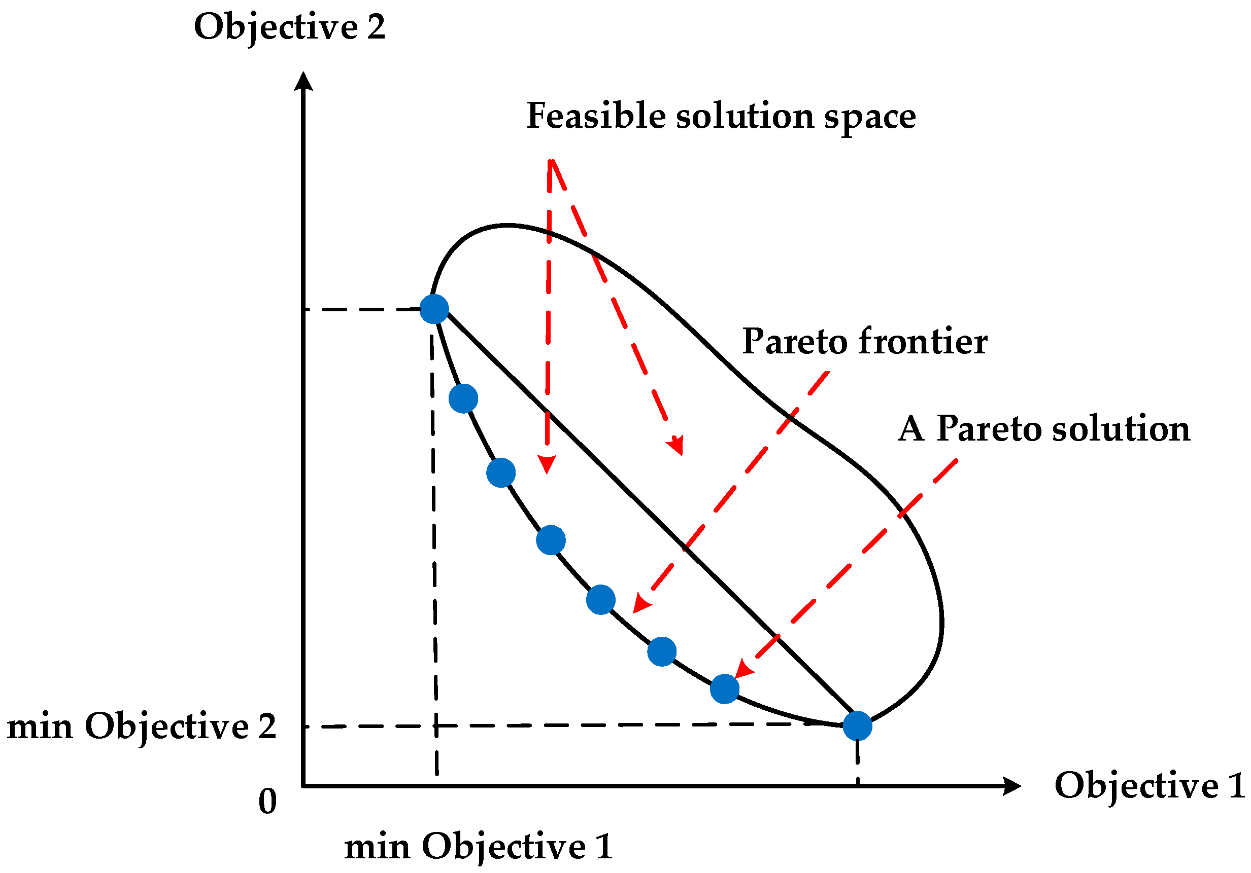
5.2. Normalized Weighted Sum Method for the Bi-Objective Optimization

Multi-objective optimization problems have two kinds of solutions, dominated solutions and Pareto solutions (non-dominated). For the multi-objective optimization with dominated solutions, its multiple objectives will reach their respective optimum simultaneously, i.e., the optimal solution for a certain objective is also the optimal one for the remaining objectives. Consequently, there only exists one optimal solution for such a multi-objective optimization. However, in most cases, the objectives in the multi-objective optimization are in mutual conflict, and the objectives cannot reach their optimum simultaneously, i.e., the respective optimal solutions for the objectives are different. There usually exists a group of solutions to such multi-objective optimization, namely Pareto solutions or non-dominated solutions. A group of Pareto solutions forms the Pareto frontier of the multi-objective optimization problem. An example of the Pareto solutions to the multi-objective optimization can be seen in Figure 1 [32]. In multi-objective decision making, with the help of the Pareto frontier of the problem, decision-makers can make a trade-off between different objectives.
There are many methods that can be utilized to generate Pareto solutions to a multi-objective optimization problem. One of the most classical and extensively used methods is the weighted sum method. In this method, different weights are distributed to the objectives, and then the weighted objectives are combined linearly to transform the multi-objective optimization problem into a single-objective one. It is a simple method that is easy to understand and utilize. Hence it has already received wide application, e.g., Xie et al. [22], Sheu [33], Samanlioglu [34], and Rakas et al. [35]. Specifically for the bi-objective optimization model constructed in this study, after weighted summation, there are:
minimize  λ 1 f 1 + λ 2 f 2
λ 1 + λ 2 = 1
0 λ 1 1
0 λ 2 1
where f 1 and f 2 represent the objective functions of minimizing the generalized costs and of minimizing the social risk along the planned routes, λ 1 and λ 2 are the distributed weights to the two objectives, and their values are determined by decision makers before model simulation. We can gain different solutions when different values are assigned to λ 1 and λ 2 , and finally generate the Pareto frontier for the problem.
In the classical weighted sum method, the objectives usually have different units and magnitudes, which will affect the optimization result when directly utilizing this method to address the multi-objective optimization problem. Consequently, in this study, we adopt an improved weighted sum method, namely the normalized weighted sum method, to solve our bi-objective optimization problem.
The normalized weighted sum method first solves the multi-objective optimization problem as a series of single-objective ones, and obtains their respective optimal solution. For the specific model in this study, let f 1 * and f 2 * separately denote the optimal values of Objective 1 and of Objective 2. After dividing by their respective optimal values, the objectives become normalized and there is no difference regarding the unit and magnitude among the different objectives. Therefore, in the normalized weighted sum method, the objective function is as below instead of as in Equation (31):
minimize  λ 1 f 1 f 1 * + λ 2 f 2 f 2 *
By using the normalized weighted sum method introduced in this section, we can generate the Pareto frontier for the case that will be discussed in the next section.

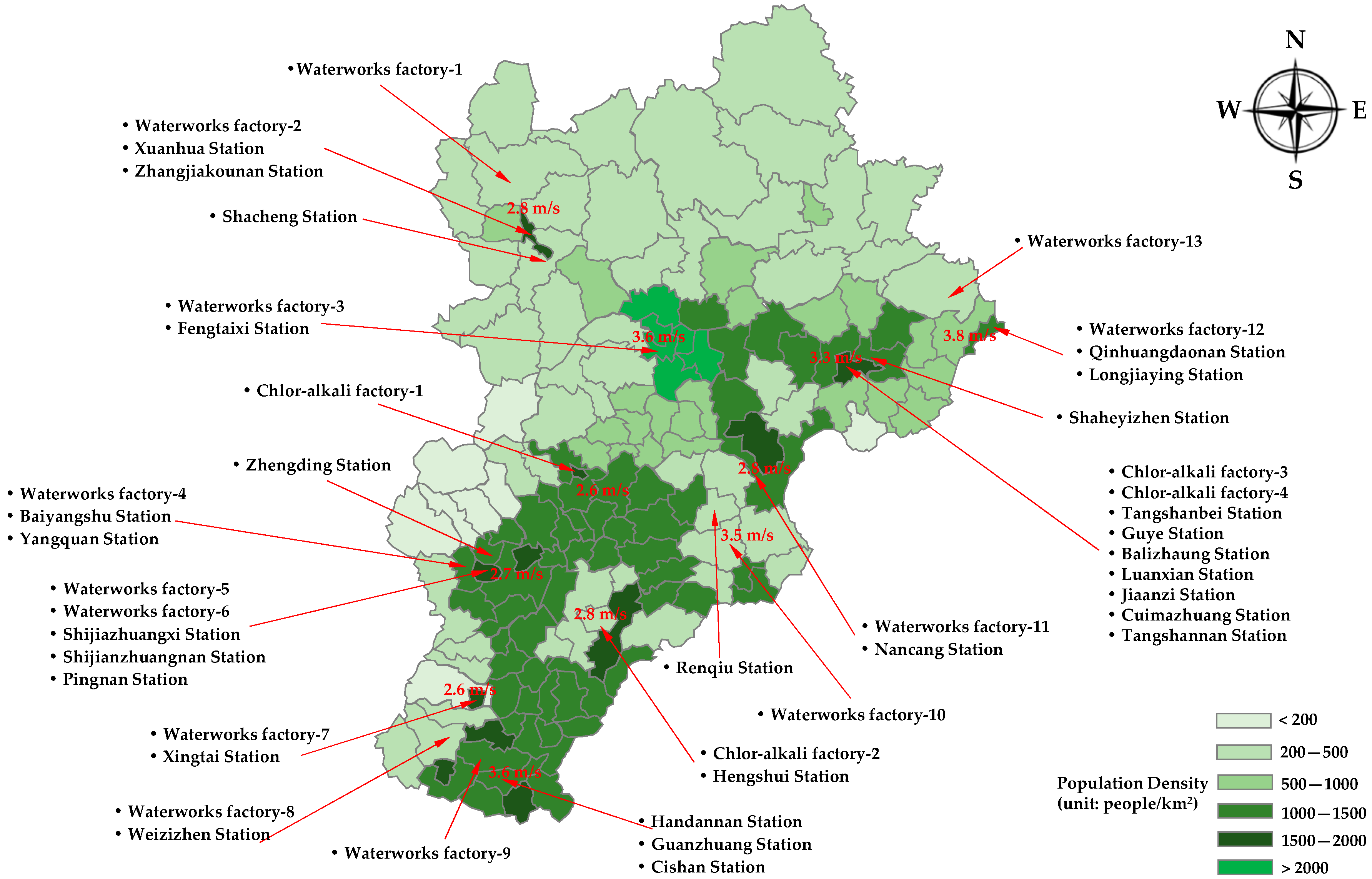
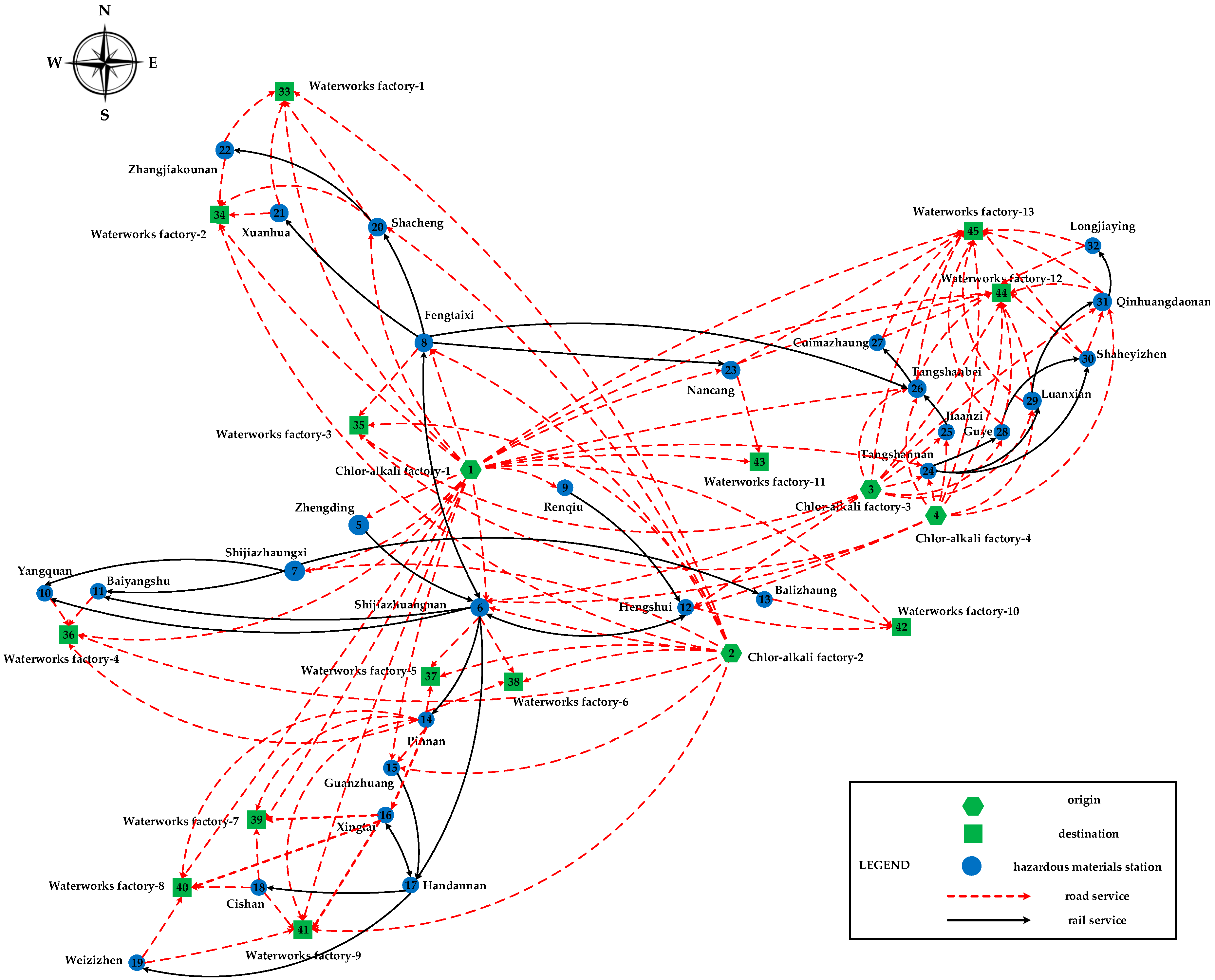
6. Empirical Case Study from the Beijing–Tianjin–Hebei Region in China

6.1. Case Description and Parameter Setting

In this section, we design an empirical case regarding liquefied chlorine transportation to demonstrate the feasibility of the proposed methods in dealing with a practical problem. The empirical case is based on a Beijing–Tianjin–Hebei Region scenario in China, in which four chlorine–alkali chemical factories in Hebei Province supply liquefied chlorine to several waterworks factories in the Beijing–Tianjin–Hebei Region. The locations of the nodes in the region are shown in Figure 2. The population density distribution and average wind speed distribution of the region are also illustrated in Figure 2. They can be used to estimate the population exposure in the empirical case.
In the large-scale empirical case, we assume that the liquefied chlorine is carried in 40-ft tank containers (in Equation (2), V O L   = 30,480 kg). The most common consequence in the liquefied chlorine transportation accidents is that the liquefied chlorine constantly releases from the damaged tank container and disperses into the surroundings as gas. This kind of accident accounts for 95% of total liquefied chlorine transportation accidents [36]. In such a transportation accident, the release of chlorine usually lasts about one hour (in Equation (2), T   = 3600 s) [37]. Therefore, according to Equation (2), when evaluating the population exposure, the release rate Q = 8.5 kg/s (8.5 × 10⁶ mg/s). The IDLH concentration threshold C ¯ in Equations (4) and (5) is 2500 mg/m3 [37]. Considering the conservative evaluation of the social risk, the atmospheric stability category is set to Level D. Consequently, in Equations (4) and (5), a   = 0.15, b   = 0.89, c   = 0.40, and d   = 0.63. Based on the information provided above, we can obtain the population exposure and environmental capacity of each node shown in Appendix B, Table B1. When evaluating the environmental capacity, in Equations (6) and (7), the allowed emissions concentration threshold C * is 80 mg/m3 according to GB 16297-1996, and the potential impact radius R *   = 8 km [38]. Therefore, the environmental capacity of each node is 85,743 tons.
The detailed topological structure of the multimodal service network for this empirical case is shown as Figure 3. It is composed of 45 nodes (including four origin nodes, 13 destination nodes, and 28 hazardous materials station nodes) and 132 directed arcs (including 31 rail service arcs and 101 road service arcs). The corresponding information on the road services in the multimodal service network is presented in Table B2. The schedules of the rail services in the multimodal service network as well as their risk parameters are given in Table B3. In Table B3, all the time data are discretized into real numbers (e.g., 10:30 on the first day is transformed into 10.5; on the second day, it is transformed into 34.5), and the same rail services operated in different periods are treated as different ones. In addition, the operation periods of all the rail services are one day/train.
The cost parameters in the road–rail multimodal routing problem of hazardous materials are stated as follows. For the rail service, its transportation unit costs can be determined by c i j s = c rail 1 + c rail 2 d i j s , where c rail  1 = 27.9 ¥/ton and c rail  2 = 0.206 ¥/ton-km. Its unit loading/unloading costs c rail   = 5.8 ¥/ton. The unit inventory costs c store   = 0.1 ¥/ton-h. The free-of-charge inventory period is 48 h. For the road service, its transportation unit costs can be determined by c i j s = c road 2 d i j s , where c road 2   = 0.76 ¥/ton-km. Its unit loading/unloading costs c road = 5.5 ¥/ton. In this empirical case, there are 25 hazardous material flows that need to be routed. Their origins, destinations, volumes, release times, and due dates are all listed in Table 1. In Table 1, the release times and due dates are all real numbers.

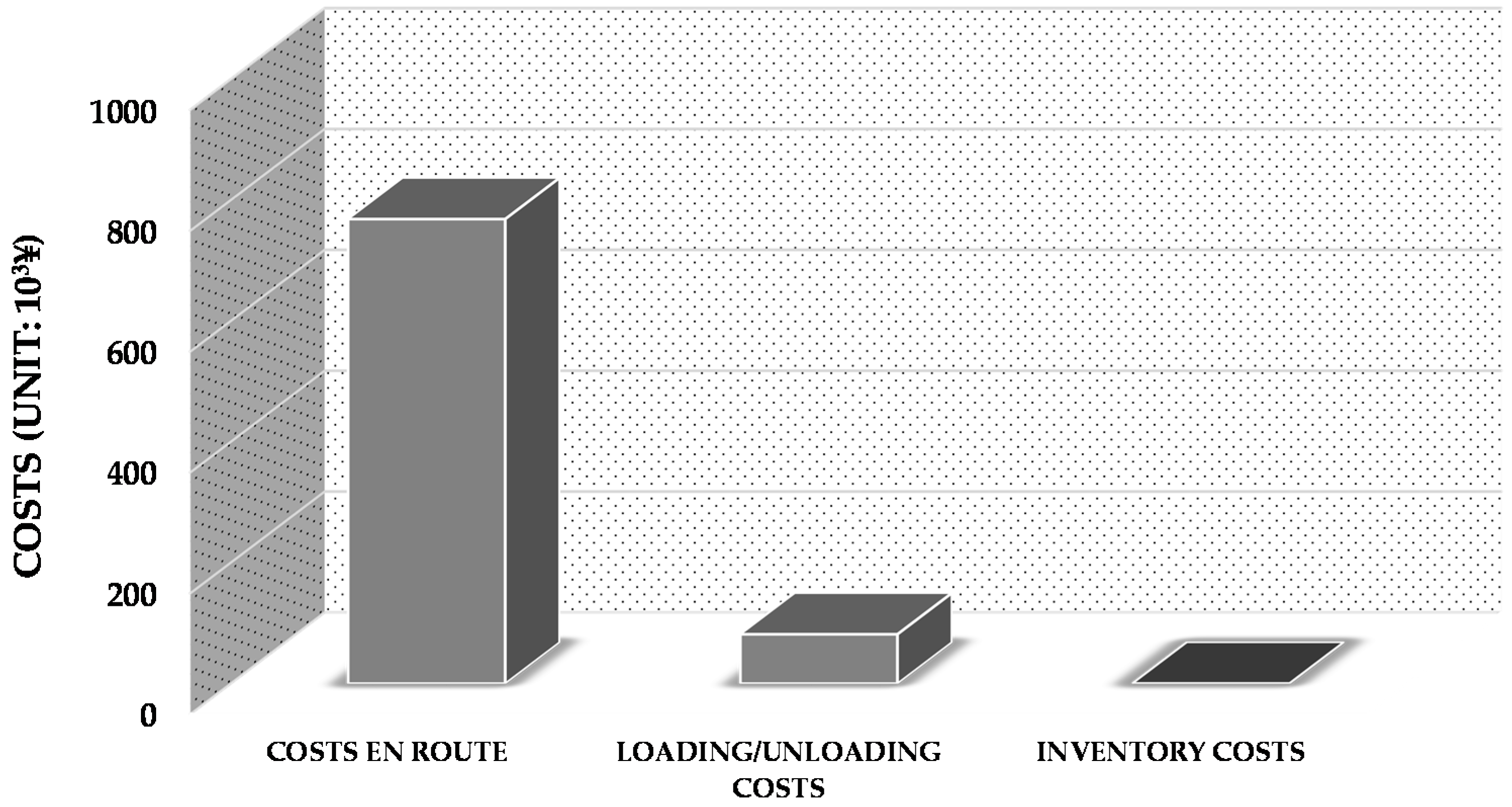
6.2. Optimization Results and Discussions

6.2.1. Simulation Environment

We set the environmental risk threshold E R max   = 0.6. Then this empirical case, which is formulated as a linear programming problem, can be solved by the exact solution algorithms. In this study, we utilize the Branch-and-Bound Algorithm to solve the specific routing problem. This algorithm is implemented by the mathematical programming software Lingo 12 (LINDO Systems Inc., Chicago, IL, USA) on a ThinkPad Laptop with Intel Core i5-5200U 2.20 GHz CPU 8 GB RAM. The scale of the empirical case problem is indicated in Table 2.

6.2.2. Multimodal Routes Illustration

First of all, we use the optimal routes with minimal generalized costs as examples to indicate how to transport hazardous materials in the road–rail multimodal service network. In this empirical case, the least-costs road–rail multimodal routes are presented in Table 3, where items such as #40103 and #32123 represent the train numbers of the rail services. As we can see from Table 3, there are two kinds of routes for the transportation of hazardous materials in the multimodal service network, including single road service routes and road–rail multimodal routes. In the latter, rail services are dominant, and road services are helpful supplements to realize the through transportation from shippers to receivers. Such routes are quite suitable for transporting hazardous materials with longer lead times.
The minimal generalized costs are 850,192 ¥ in this empirical case. The structure of these costs is shown in Figure 4. As we can see from Figure 4, costs en route account for the majority of the total generalized costs (in this case, approximately 90%). The planning horizon of the empirical case is limited; the inventory times of the hazardous materials are hence shorter than the free-of-charge inventory period. Consequently, as for this empirical case, there are no inventory costs in the minimal generalized costs.

6.2.3. Single-Objective Scenarios

First we address the two single-objective optimization problems that separately aim at minimizing the total generalized costs (unit: ¥) and the social risk (unit: 104 people-ton). The respective optimal solutions to the three objectives are given in Table 4. Table 4 clearly indicates that the two objectives cannot reach their respective optimal values simultaneously, i.e., the optimal solution to a certain objective is not the optimal one for the remaining objective. Therefore, there exist Pareto solutions for the bi-objective optimization problem.

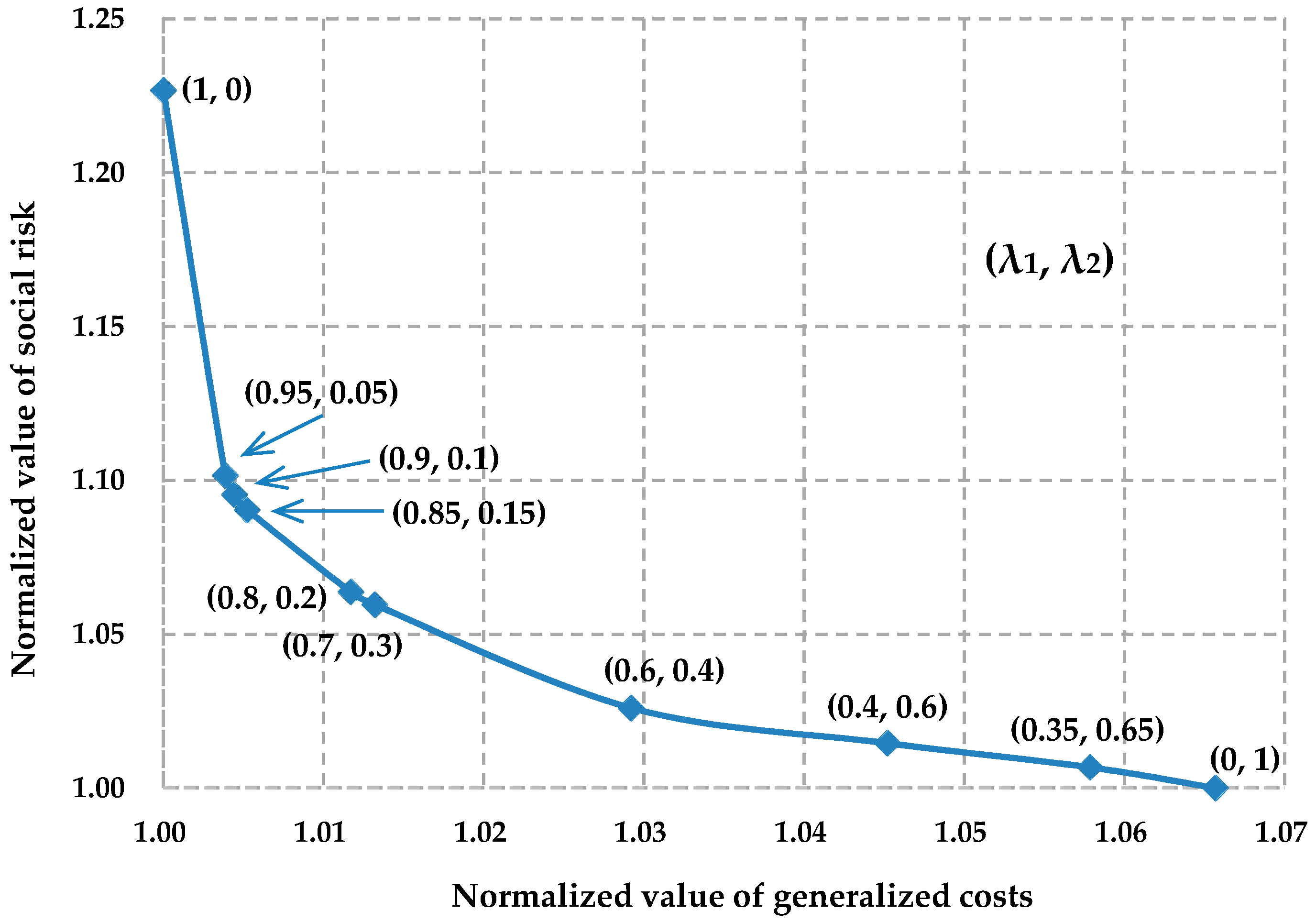
6.2.4. Bi-Objective Scenario

In bi-objective decision making, because the two objectives are conflicting, decision-makers should make a trade-off between lowering the generalized costs and reducing the social risk. By using the normalized weighted sum method introduced in Section 5, we can generate Pareto solutions (Pareto frontier) to the bi-objective optimization problem as in Figure 5. Figure 5 shows that improving the economy of the multimodal routing will lead to an increase in the social risk along the planned routes, and reducing the social risk along the planned routes will lower the economy of the multimodal routing.
Figure 5 provides various candidate solutions to the bi-objective optimization problem that will be helpful for decision-makers trying to balance the conflict between cost objectives and risk objectives. For example, in the trade-off between generalized costs and social risk, if decision-makers consider that it is acceptable as long as the normalized social risk is lower than 1.05, then the last four Pareto solutions in Figure 5 can be their candidate multimodal route schemes. Considering minimization of the generalized costs, decision-makers will finally select the multimodal route corresponding to the 7th Pareto solution to transport the hazardous materials.

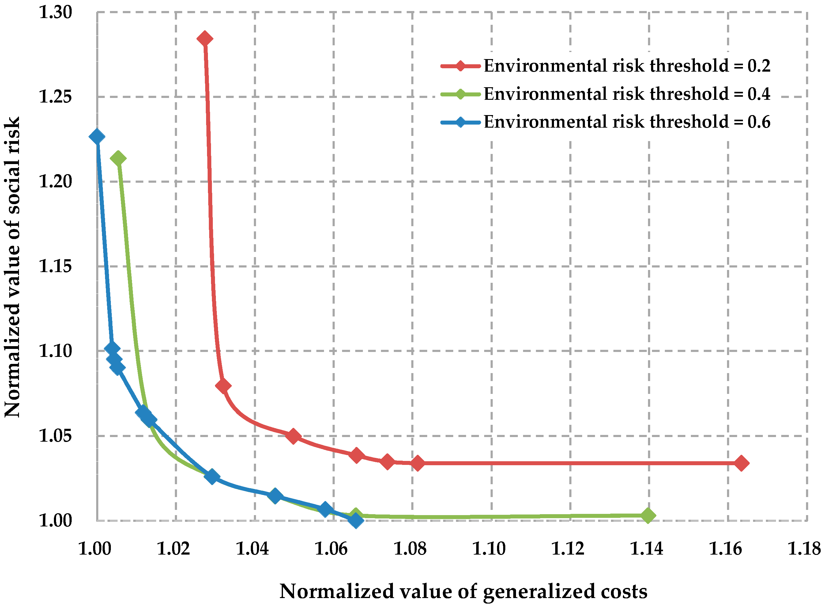
6.2.5. Sensitivity of the Pareto Solutions with Respect to the Environmental Risk Threshold

In this section, we conduct sensitivity analysis of the Pareto solutions with respect to the environmental risk threshold. Because the minimal environmental risk in the multimodal service network is 0.135, we generate three Pareto frontiers corresponding to the thresholds 0.2, 0.4, and 0.6. Figure 6 shows the variation of the Pareto frontiers when the environmental risk threshold increases. In Figure 6, the generalized costs and social risk are separately normalized by 850,192 and 506,362, which are the optimal values of generalized costs and social risk, respectively, when the environmental risk threshold is 0.6.
As we can see from Figure 6, the Pareto frontier of the bi-objective optimization problem will move to the left with the increase of the environmental risk threshold. That is to say, we can lower the generalized costs and the social risk simultaneously if we relax the environmental risk constraint by enlarging the environmental risk threshold. The extrapolated Figure 6 can also provide a reference for decision-makers when they are not sure of the setting of the environmental risk threshold for the multimodal service network.

7. Conclusions

In this study, we explore the road–rail multimodal routing problem of hazardous materials from the operational level of network planning. The main contribution made in this study is its comprehensive formulation of the following characteristics, so that the specific routing problem can be addressed from an improved practical viewpoint: (1) specific customer demands from transportation economy and efficiency; (2) multiple hazardous materials flows; (3) railway schedule-based space–time constraints; (4) environmental risk constraint; and (5) bi-objective optimization from the viewpoint of generalized costs vs. social risk management. Consideration of all these formulation characteristics significantly enhances the feasibility of the proposed model in dealing with practical problems, which is also a good development of current studies on the routing problem of hazardous materials.
Besides the improvement in model formulation, this study also develops concise linear reformulations that transform the initial nonlinear model into its equivalent linear programming. On the one hand, the linear reformulations enable the problem to be solved effectively by an exact solution algorithm that can be easily implemented by standard mathematical programming software. On the other hand, the linearization method can also provide an exact benchmark in order to systematically test the performance of various heuristic algorithms in dealing with the specific routing problem. In addition, the exact solution algorithm, e.g., the Branch-and-Bound Algorithm, can also test whether the model itself is mathematically logical or not.
In this large-scale empirical case study, by using the Branch-and-Bound Algorithm in Lingo 12, the optimal solution for a certain scenario can be generated within 3 min. Although the computational time for a single solution is acceptable, a large amount of computational time will be consumed when several Pareto solutions are required and a sensitivity analysis needs to be conducted. Therefore, it is still necessary to design a heuristic algorithm to address the problem more efficiently. Consequently, our further study will focus on the design of the heuristic algorithm. As claimed above, this study has provided an exact benchmark for testing the heuristic algorithm, which has provided a solid foundation for us to carry on such a study.

Acknowledgments

This study was supported by the National Natural Science Foundation Project of China (No. 71390332-3) and a Scientific Research Developing Project of the China Railway Corporation (No. 2014X009-B). The authors would also like to thank Cyril Bernard Lucas from the United Kingdom, author of the book Atomic and Molecular Beams: Production and Collimation, for his great contributions in helping us edit and polish the language of this paper.

Author Contributions

Yan Sun constructed the mathematical model, designed the solution strategy, conducted the empirical case experiment, and wrote the paper. Maoxiang Lang thoroughly reviewed and improved the paper. Danzhu Wang participated in the Lingo simulation in the case study. All authors have discussed and contributed to the manuscript. All authors have read and approved the final manuscript.

Conflicts of Interest

The authors declare no conflict of interest.

Appendix A. Model Linear Reformulation

  • Reformulation 1. By using a non-negative variable U i k to replace the nonlinear function max { h δ ( i ) r Γ h i X h i r k + j δ + ( i ) s Γ i j X i j s k 1 ,   0 } and adding two linear Equations (A2) and (A3), nonlinear Component (11) in Objective 1 can be reformulated as a linear function (A1).
    k K i N ( j δ + ( i ) s S i j c s q k X i j s k + h δ ( i ) r S h i c r q k X h i r k ) k K i N \ { o k ,   d k   } ( 2 c rail q k U i k )
    U i k h δ ( i ) r Γ h i X h i r k + j δ + ( i ) s Γ i j X i j s k W i k   k K ,   i N \ { o k ,   d k   }
    U i k 0   k K ,   i N \ { o k ,   d k   }
U i k has the same function of max { h δ ( i ) r Γ h i X h i r k + j δ + ( i ) s Γ i j X i j s k 1 ,   0 } . If and only if U i k   = 1, there ought to be no loading and unloading costs for hazardous materials k at node i , and the extra loading and unloading costs contained in k K i N ( j δ + ( i ) s S i j c s q k X i j s k + h δ ( i ) r S h i c r q k X h i r k ) should be deducted. The following explanation proves that U i k is equivalent to max { h δ ( i ) r Γ h i X h i r k + j δ + ( i ) s Γ i j X i j s k 1 ,   0 } .
There are three independent cases in Component (11):
(i)
Hazardous materials k get transshipped between rail services at node i , i.e., h δ ( i ) r Γ h i X h i r k = 1 and j δ + ( i ) s Γ i j X i j s k = 1, in this case, max { h δ ( i ) r Γ h i X h i r k + j δ + ( i ) s Γ i j X i j s k 1 ,   0 }   = 1.
(ii)
Hazardous materials k get transshipped between road service and rail service at node i , i.e., h δ ( i ) r Γ h i X h i r k   =1 and j δ + ( i ) s Γ i j X i j s k = 0 or h δ ( i ) r Γ h i X h i r k = 0 and j δ + ( i ) s Γ i j X i j s k   = 1, in this case, max { h δ ( i ) r Γ h i X h i r k + j δ + ( i ) s Γ i j X i j s k 1 ,   0 }   = 0.
(iii)
Node i is not covered in the route of hazardous materials k , i.e., h δ ( i ) r Γ h i X h i r   k = 0 and j δ + ( i ) s Γ i j X i j s k   = 0, in this case, max { h δ ( i ) r Γ h i X h i r k + j δ + ( i ) s Γ i j X i j s k 1 ,   0 }   = 0.
For Case (i), obviously, W i k   = 1, and U i k 1 according to Equation (A2). Then Equation (A3) and the minimization of Component (A1) will restrict U i k   = 1. For Case (ii), W i k   = 1 also exists, and U i k 0 according to Equation (A2). Due to the restriction of Equation (A3), U i k   = 0. For Case (iii), W i k   = 0, similarly to Case ii, U i k will finally equal to 0. Above all, when inputting the same cases into Equations (32)~(34), U i k will contribute the same results to max  { h δ ( i ) r Γ h i X h i r k + j δ + ( i ) s Γ i j X i j s k 1 ,   0 } . Consequently, the equivalency above is verified.
  • Reformulation 2. By using a non-negative decision variable V i j s k to replace the nonlinear function Z i j s k h δ ( i ) r Ω i j X h i r k and adding two linear Equations (A5) and (A6), the nonlinear Component (12) in Objective 1 can be reformulated as a linear function (A4).
    k K ( i , j ) A s Γ i j c store q k V i j s k
    V i j s k Z i j s k + M ( h δ ( i ) r Ω i j X h i r k 1 )   k K ,   ( i , j ) A ,   s Γ i j
    V i j s k 0   k K ,   ( i , j ) A ,   s Γ i j
In this reformulation, the following two cases obviously exist, which proves the equivalency above.
(i)
If h δ ( i ) r Ω i j X h i r k = 0, i.e., hazardous materials k arrive at node i by the rail service, there are V i j s k M and V i j s k 0 according to Equations (A5) and (A6), and the minimization of Component (A4) will restrict V i j s k   = 0, which matches the setting that there are no inventory costs at the node if the hazardous materials are transshipped between different rail services.
(ii)
If h δ ( i ) r Ω i j X h i r k = 1, i.e., hazardous materials k arrive at node i by road service, there are V i j s k Z i j s k and V i j s k 0 , and minimization of Component (A4) will restrict V i j s k = Z i j s k , which matches the setting that inventory costs will be charged at the node according to the charged inventory time if the hazardous materials are transshipped from road service to rail service.
  • Reformulation 3. Nonlinear Equation (21) is equivalent to linear Equation (A7) as follows.
    Y i k u i s ( X i j s k + h δ ( i ) s Ω i j X h i r k 1 ) + f i s ( X i j s k + h δ ( i ) s Γ i j X h i r k 1 ) + M ( 1 X i j s k )   ( i ,   j ) A ,   s Γ i j
It is obvious that we can gain the same results as Equation (21) after we separately input the three given cases, Case (i)–Case (iii), from Equation (21) into Equation (A7). Therefore, the two constraints are equivalent to each other.
  • Reformulation 4. Nonlinear Equations (23), (24) and (26) are separately equivalent to linear Equations (A8)–(A13). For detailed proofs of the above three equivalencies, readers can refer to our previous study [26].
    Y i k + t i j s Y j k M ( X i j s k 1 )   k K ,   ( i , j ) A ,   s Ω i j
    Y i k + t i j s Y j k M ( 1 X i j s k )   k K ,   ( i , j ) A ,   s Ω i j
    l i s j δ + ( i ) s Ω i j X i j s k + e i s j δ + ( i ) s Γ i j X i j s k Y i k M ( X h i r k 1 )   k K ,   ( h , i ) A ,   r Γ h i
    l i s j δ + ( i ) s Ω i j X i j s k + e i s j δ + ( i ) s Γ i j X i j s k Y i k M ( 1 X h i r k )   k K ,   ( h , i ) A ,   r Γ h i
    Z i j s k M ( X i j s k 1 ) + ( l i s Y i k τ )   k K ,   ( i , j ) A ,   s Γ i j
    Z i j s k M X i j s k   k K ,   ( i , j ) A ,   s Γ i j

Appendix B

Table B1. Population exposures around the nodes in the empirical case.
NodePopulation Exposure (Unit: 104 People)NodePopulation Exposure (Unit: 104 People)NodePopulation Exposure (Unit: 104 People)
13.44162.87311.74
20.66171.32321.74
32.29180.58330.50
42.29190.58342.48
52.31200.66353.56
62.13212.48362.13
72.84222.48372.84
83.56232.32382.84
90.32242.29392.87
102.13252.29400.58
112.13262.29411.12
120.66272.29420.43
132.29282.29432.32
142.13292.29441.74
151.32301.69450.82
Table B2. Transportation distances, times, and risk parameters for road services in the large-scale empirical example.
ArcDistance (Unit: km)Time (Unit: h)Population Exposure (Unit: 104 People)Environmental Capacity (Unit: 104 Ton)ArcDistance (Unit: km)Time (Unit: h)Population Exposure (Unit: 104 People)Environmental Capacity (Unit: 104 Ton)
(1, 5)1291.857.177.47(4, 26)80156.724.64
(1, 6)1532.381.368.86(4, 29)1081.876.576.26
(1, 7)162296.929.39(4, 45)2152.8117.4712.46
(1, 8)1481.862.318.57(6, 37)80.26.740.46
(1, 9)901.552.425.27(6, 38)100.38.420.58
(1, 15)2432.8123.8414.08(8, 35)30.23.990.17
(1, 20)2353.357.2813.62(10, 36)90.44.390.52
(1, 23)1742.561.6910.08(11, 36)80.33.900.46
(1, 24)2913.477.3716.86(12, 42)152272.418.81
(1, 26)3083.776.4317.84(13, 42)150.66.480.87
(1, 33)403598.2223.35(14, 15)1011.449.235.85
(1, 34)2483.363.7414.37(14, 16)1231.731.677.13
(1, 36)2383.2137.1113.79(14, 36)1141.875.786.60
(1, 39)2623.3156.7415.18(14, 37)90.45.580.52
(1, 40)3824.2169.2822.13(14, 38)90.45.580.52
(1, 41)3333.8162.3219.29(14, 39)1191.965.926.89
(1, 42)1642.383.589.50(14, 40)2392.7119.6813.85
(1, 43)1712.364.419.91(14, 41)1912.463.4811.07
(1, 44)4344.9211.5625.15(16, 39)60.23.990.35
(1, 45)4455.4226.7825.78(16, 40)1431.822.188.29
(2, 6)1501.876.448.69(16, 41)951.543.365.50
(2, 7)1511.776.958.75(18, 39)711.615.104.11
(2, 8)2656131.5215.35(18, 40)560.89.933.24
(2, 12)30.30.400.17(18, 41)45113.962.61
(2, 15)1502.166.478.69(19, 40)751.113.294.35
(2, 20)3774.5125.3021.84(19, 41)1612.146.848.75
(2, 33)5776.6145.7433.43(20, 33)2152.6100.0412.46
(2, 34)4225.2114.0724.45(20, 34)59141.833.42
(2, 35)2653131.5215.35(21, 33)1682.272.219.73
(2, 36)2373119.5213.73(21, 34)40.12.390.21
(2, 37)1551.978.998.98(22, 33)1131.948.576.55
(2, 38)1401.871.358.11(22, 34)230.515.291.33
(2, 41)2562.8113.4414.83(23, 43)80.33.370.46
(3, 6)4394.8184.8125.43(23, 44)2663.1126.1315.41
(3, 12)3764.4159.9621.78(23, 45)2784.2123.1916.11
(3, 24)230.617.841.33(26, 44)1371.677.717.94
(3, 25)100.37.760.58(26, 45)1492.281.418.63
(3, 26)270.719.141.56(27, 44)1401.779.418.11
(3, 28)170.416.870.98(27, 45)1522.283.058.81
(3, 29)42132.572.43(28, 44)1261.676.777.30
(3, 31)1441.973.388.34(28, 45)1382.170.338.00
(3, 35)2012.7172.8011.65(29, 44)1011.558.955.85
(3, 44)1421.880.558.23(29, 45)1012.261.545.85
(3, 45)1542.384.148.92(30, 31)971.559.105.62
(4, 6)4124.4173.4523.87(30, 44)951.357.895.50
(4, 12)3594.4152.7220.80(30, 45)1071.759.276.20
(4, 24)590.841.833.42(31, 44)70.36.200.41
(4, 25)74152.474.29(31, 45)1311.7101.597.59
(4, 31)1712.196.999.91(32, 44)140.512.410.81
(4, 35)2042.8175.3811.82(32, 45)1421.8100.688.23
(4, 44)1691.9145.299.79
Table B3. Schedules and risk parameters of the rail services in the multimodal service network.
Train No.4750147503475054750721018210202102221024210263402934035
Origin55556666666
Loading start time20.42.810.615.11.60.83.1610.31.55.8
Loading cutoff time20.93.811.515.83.12.34.67.511.837.3
Classification start time20.73.511.315.62.62.84.56.510.826.3
Classification cutoff time21.2412.216.23.63.85.1812.33.57.8
Departure time21.44.312.616.54.14.35.68.512.848.3
Destination6666888881010
Arrival time22.35.113.417.41818.418.718.819.57.510.8
Disassembly start time22.55.313.617.718.518.919.218.319710.3
Disassembly cutoff time235.714.218.42020.520.720218.512
Unloading start time22.85.514181919.419.719.820.58.511.8
Unloading cutoff time23.5614.51920.52121.221.3221013.3
Distance (unit: km)17171717273273273273273115115
Capacity (unit: ton)70689499476219731354118115411668799994
Population exposure (unit: 104 people)9.869.869.869.86146.59146.59146.59146.59146.5964.2264.22
Environmental capacity (unit: 104 ton)13.6713.6713.6713.67219.45219.45219.45219.45219.4592.4492.44
Train No.3404734055340013404547551475554755732101321053210932119
Origin66666666666
Loading start time9.311.816.18.617.95.511.716.317.117.32.8
Loading cutoff time10.813.317.610.118.46.212.317.818.618.84.3
Classification start time9.812.316.69.118.3611.916.817.617.83.3
Classification cutoff time11.313.818.110.618.66.512.418.319.119.34.8
Departure time11.814.318.611.118.96.912.718.819.619.85.3
Destination1010111114141417171717
Arrival time14.316.82113.519.1712.821.422.522.97.5
Disassembly start time13.816.320.51319.47.513.220.92222.47
Disassembly cutoff time15.51822.314.719.9813.722.423.8248.7
Unloading start time15.317.82214.5207.813.522.423.523.98.5
Unloading cutoff time16.819.323.516218.51423.92525.410
Distance (unit: km)115115107107999162162162162
Capacity (unit: ton)106617471062109487410809721680118111451786
Population exposure (unit: 104 people)64.2264.2259.7559.754.254.254.2580.0380.0380.0380.03
Environmental capacity (unit: 104 ton)92.4492.4486.0186.017.237.237.23130.22130.22130.22130.22
Train No.3212330002300043000634005340113403734041340493401334025
Origin66667777777
Loading start time6.816.717.418.318.320.16.67.810.321.41.6
Loading cutoff time8.318.218.919.819.821.68.19.311.822.93.1
Classification start time7.317.217.918.818.820.67.18.310.821.92.1
Classification cutoff time8.818.719.420.320.322.18.69.812.323.43.6
Departure time9.319.219.920.820.822.69.110.312.823.94.1
Destination1712121210101010101111
Arrival time11.921.522.223.1230.811.312.41526.1
Disassembly start time11.42121.722.622.50.310.811.914.51.55.6
Disassembly cutoff time1322.823.524.324.6212.513.516.73.37.3
Unloading start time12.922.523.224.1241.812.313.41637.1
Unloading cutoff time14.42424.725.625.53.313.814.917.54.58.6
Distance (unit: km)1621211211211071071071071079999
Capacity (unit: ton)100115051109150819878281134172718369401620
Population exposure (unit: 104 people)80.0353.6953.6953.6959.7559.7559.7559.7559.7555.2855.28
Environmental capacity (unit: 104 ton)130.2297.2697.2697.2686.0186.0186.0186.0186.0179.5879.58
Train No.3403133912339142100121017210192102321025210273303933041
Origin77788888888
Loading start time3.620.40.419.12.53.54.16.811.118.520.5
Loading cutoff time5.121.91.120.6455.68.312.62022
Classification start time4.120.90.119.6344.67.311.61921
Classification cutoff time5.622.41.621.14.55.56.18.813.120.522.5
Departure time6.122.92.121.6566.69.313.62123
Destination1113136666662020
Arrival time8.23.35.25.711.313.515.320.50.722.90.9
Disassembly start time7.72.84.75.210.81314.8200.222.40.4
Disassembly cutoff time9.54.66.3712.714.516.621.6223.92
Unloading start time9.24.36.26.712.314.516.321.51.723.91.9
Unloading cutoff time10.75.87.78.213.81617.8233.225.43.4
Distance (unit: km)99185185273273273273273273121121
Capacity (unit: ton)1469117412531840199011461075139314951170922
Population exposure (unit: 104 people)55.2875.4975.49146.59146.59146.59146.59146.59146.5933.2633.26
Environmental capacity (unit: 104 ton)79.58148.71148.71219.45219.45219.45219.45219.45219.4597.2697.26
Train No.3305733061330673554735553355573550538001380113802740103
Origin88888888889
Loading start time810.114.512.713.614.918.616.3113.715.9
Loading cutoff time9.511.61614.215.116.420.117.82.515.216.4
Classification start time8.510.61513.214.115.419.116.81.514.216.1
Classification cutoff time1012.116.514.715.616.920.618.3315.716.9
Departure time10.512.61715.216.117.421.118.83.516.217.3
Destination2020212323232326262612
Arrival time12.414.42016.818.619.223.721.362120.6
Disassembly start time11.913.919.516.318.118.723.220.85.520.521
Disassembly cutoff time13.515.721.2182020.524.722.5722.321.6
Unloading start time13.415.42117.819.620.224.722.372221.4
Unloading cutoff time14.916.922.519.321.121.726.223.88.523.522
Distance (unit: km)121121171113113113113262262262127
Capacity (unit: ton)1546994110294412391462100985614841135864
Population exposure (unit: 104 people)33.2633.2649.2182.5282.5282.5282.52225.09225.09225.0994.54
Environmental capacity (unit: 104 ton)97.2697.26137.4690.8390.8390.8390.83210.61210.61210.61102.09
Train No.3000130003300054008147405474063910139109391113911339115
Origin1212121516171717171717
Loading start time23.15.57.117.722.514.217.35.58.211.514.7
Loading cutoff time24.678.619.22415.718.879.71316.2
Classification start time23.667.618.22314.717.868.71215.2
Classification cutoff time25.17.59.119.724.516.219.37.510.213.516.7
Departure time25.689.620.22516.719.8810.71417.2
Destination6661717161818181818
Arrival time28.110.812.122.325.917.621.29.412.215.418.7
Disassembly start time27.610.311.621.825.417.120.78.911.714.918.2
Disassembly cutoff time29.51213.723.52718.822.210.513.616.420
Unloading start time29.111.813.123.326.918.622.210.413.216.419.7
Unloading cutoff time30.613.314.624.828.420.123.711.914.717.921.2
Distance (unit: km)12112126752524444444444
Capacity (unit: ton)190188413928571893110720111892146912421058
Population exposure (unit: 104 people)55.415.495.4931.6620.1020.1011.3420.7920.7920.7920.79
Environmental capacity (unit: 104 ton)97.269.659.6553.8641.8041.8035.3735.3735.3735.3735.37
Train No.3918139183391853320133203467214672382114/386662/14691546947
Origin1717172020242424242525
Loading start time22.71.513.718.31.922.54.82.57.98.65
Loading cutoff time24.2315.219.83.4235.449.49.25.7
Classification start time23.2214.218.82.4235.238.48.95.5
Classification cutoff time24.73.515.720.33.923.564.59.99.66.2
Departure time25.2416.220.84.423.86.4510.4106.5
Destination1919192222282829302626
Arrival time34.814.70.722.25.81.47712.810.57
Disassembly start time34.314.20.221.75.31.87.56.512.310.87.2
Disassembly cutoff time3615.91.923.472.88.18.21411.57.8
Unloading start time35.815.71.723.26.82.17.8813.811.47.5
Unloading cutoff time37.317.23.224.78.338.59.515.3128.1
Distance (unit: km)2032032037575262649691313
Capacity (unit: ton)7221284167511561786102311111987150911601283
Population exposure (unit: 104 people)52.3252.3252.3245.1045.1018.9918.9935.7835.579.499.49
Environmental capacity (unit: 104 ton)163.18163.18163.1860.2960.2920.9020.9039.3955.4710.4510.45
Train No.4695146944468214682946833468354683943093469814698346981
Origin2526282828282829313131
Loading start time211.218.53.97.58.61110.9207.519.5
Loading cutoff time21.7219.24.58.39.41211.6218.621
Classification start time21.91.8194.28911.511.220.88.420.7
Classification cutoff time22.32.419.558.81012.41221.79.221.6
Departure time22.52.719.75.48.110.312.612.6229.622
Destination2627303030303031323232
Arrival time233.120.46.28.91113.31422.712.422.7
Disassembly start time23.33.5216.59.111.413.714.53012.823
Disassembly cutoff time23.94.121.57.19.812.314.415.230.81423.8
Unloading start time23.73.921.46.79.511.71414.830.413.423.4
Unloading cutoff time24.24.622.27.510.412.71515.831.41524.2
Distance (unit: km)138535353535388101010
Capacity (unit: ton)8791930103621437781456122016961987972762
Population exposure (unit: 104 people)9.495.8427.3227.3227.3227.3227.3245.364.944.944.94
Environmental capacity (unit: 104 ton)10.456.4342.6042.6042.6042.6042.6070.748.048.048.04

References

  1. Zhao, J.; Huang, L.X.; Lee, D.H.; Peng, Q.Y. Improved approaches to the network design problem in regional hazardous waste management systems. Transp. Res. Part E Logist. Transp. Rev. 2016, 8, 52–75. [Google Scholar] [CrossRef]
  2. Tarantilis, C.D.; Kiranoudis, C.T. Using the vehicle routing problem for the transportation of hazardous materials. Oper. Res. 2001, 1, 67–78. [Google Scholar] [CrossRef]
  3. Bubbico, R.; Maschio, G.; Mazzarotta, B.; Milazzo, M.F.; Parisi, E. Risk management of road and rail transport of hazardous materials in Sicily. J. Loss Prev. Proc. 2006, 19, 32–38. [Google Scholar] [CrossRef]
  4. Chu, Q.Z.; Zhang, J.Y.; Xie, Z.Q. Road Network Design for Hazardous Materials Transportation Based on Bi-level Programming. J. Chongqing Jiaotong Univ. (Nat. Sci.) 2010, 29, 597–603. [Google Scholar]
  5. Wu, Z.Z.; Zhang, S.Z.; Zhang, Y.; Shi, C.; Liu, N.; Yang, G.L. Statistical analysis of hazardous chemicals accidents occurring in China during 2006–2010. J. Saf. Sci. Technol. 2011, 7, 5–9. [Google Scholar]
  6. Ren, C.X.; Wu, Z.Z. Probe into methods of optimal road transportation routing for hazardous materials. China Saf. Sci. J. 2006, 16, 129–134. [Google Scholar]
  7. Androutsopoulos, K.N.; Zografos, K.G. Solving the bicriterion routing and scheduling problem for hazardous materials distribution. Transp. Res. Part C Emerg. Technol. 2010, 18, 713–726. [Google Scholar] [CrossRef] [Green Version]
  8. List, G.F.; Mirchandani, P.B.; Turnquist, M.A.; Zografos, K.G. Modeling and analysis for hazardous materials transportation: Risk analysis, routing/scheduling and facility location. Transp. Sci. 1991, 25, 100–114. [Google Scholar] [CrossRef]
  9. Ren, C.X.; Wu, Z.Z. On route-choice analysis of hazardous materials transportation. J. Saf. Environ. 2006, 6, 84–88. [Google Scholar]
  10. Verter, V.; Kara, B.Y. A path-based approach for hazmat transport network design. Manag. Sci. 2008, 54, 29–40. [Google Scholar] [CrossRef]
  11. Erkut, E.; Gzara, F. Solving the hazmat transport network design problem. Comput. Oper. Res. 2008, 35, 2234–2247. [Google Scholar] [CrossRef] [Green Version]
  12. Kara, B.Y.; Verter, V. Designing a road network for hazardous materials transportation. Transp. Sci. 2004, 38, 188–196. [Google Scholar] [CrossRef]
  13. Erkut, E.; Alp, O. Designing a road network for hazardous materials shipments. Comput. Oper. Res. 2007, 34, 1389–1405. [Google Scholar] [CrossRef]
  14. Boyer, O.; Sai Hong, T.; Pedram, A.; Mohd Yusuff, R.B.; Zulkifli, N. A mathematical model for the industrial hazardous waste location-routing problem. J. Appl. Math. 2013, 2013, 1–10. [Google Scholar] [CrossRef]
  15. Alumur, S.; Kara, B.Y. A new model for the hazardous waste location-routing problem. Comput. Oper. Res. 2007, 34, 1406–1423. [Google Scholar] [CrossRef]
  16. Zhao, J.; Verter, V. A bi-objective model for the used oil location-routing problem. Comput. Oper. Res. 2015, 62, 157–168. [Google Scholar] [CrossRef]
  17. Shuai, B.; Zhao, J. Bi-objective 0–1 linear programming model for combined location–routing problem in hazardous waste logistics system. J. Southwest Jiaotong Univ. 2011, 46, 326–332. [Google Scholar]
  18. Helander, M.E.; Melachrinoudis, E. Facility location and reliable route planning in hazardous material transportation. Transp. Sci. 1997, 31, 216–226. [Google Scholar] [CrossRef]
  19. Giannikos, I. A multiobjective programming model for locating treatment sites and routing hazardous wastes. Eur. J. Oper. Res. 1998, 104, 333–342. [Google Scholar] [CrossRef]
  20. Zografros, K.G.; Samara, S. Combined location-routing model for hazardous waste transportation and disposal. Transp. Res. Rec. J. Transp. Res. Board 1989, 1245, 52–59. [Google Scholar]
  21. Bubbico, R.; Di Cave, S.; Mazzarotta, B. Risk analysis for road and rail transport of hazardous materials: A simplified approach. J. Loss Prevent. Proc. 2004, 17, 477–482. [Google Scholar] [CrossRef]
  22. Xie, Y.; Lu, W.; Wang, W.; Quadrifoglio, L. A multimodal location and routing model for hazardous materials transportation. J. Hazard. Mater. 2012, 227, 135–141. [Google Scholar] [CrossRef] [PubMed]
  23. Jiang, Y.; Zhang, X.; Rong, Y.; Zhang, Z. A Multimodal Location and Routing Model for Hazardous Materials Transportation based on Multi-commodity Flow Model. Procedia-Soc. Behav. Sci. 2014, 138, 791–799. [Google Scholar] [CrossRef]
  24. Verma, M.; Verter, V. A lead-time based approach for planning rail–truck intermodal transportation of dangerous goods. Eur. J. Oper. Res. 2010, 202, 696–706. [Google Scholar] [CrossRef]
  25. Verma, M.; Verter, V.; Zufferey, N. A bi-objective model for planning and managing rail-truck intermodal transportation of hazardous materials. Transp. Res. Part E Logist. Transp. Rev. 2012, 48, 132–149. [Google Scholar] [CrossRef]
  26. Sun, Y.; Lang, M.X. Modeling the Multicommodity Multimodal Routing Problem with Schedule-Based Services and Carbon Dioxide Emission Costs. Math. Probl. Eng. 2015, 2015, 406218. [Google Scholar] [CrossRef]
  27. Erkut, E.; Tjandra, S.A.; Verter, V. Hazardous materials transportation. In Handbooks in Operations Research and Management Science; Elsevier: Amsterdam, The Netherlands, 2007; Volume 14, pp. 539–621. [Google Scholar]
  28. Ding, X.W.; Wang, S.L.; Xu, G.Q. A review of studies on the discharging dispersion of flammable and toxic gases. Chem. Ind. Eng. 1999, 16, 118–122. [Google Scholar]
  29. Verma, M.; Verter, V. Railroad transportation of dangerous goods: Population exposure to airborne toxins. Comput. Oper. Res. 2007, 34, 1287–1303. [Google Scholar] [CrossRef]
  30. Zhao, J. The Location-Routing Problem of Hazardous Waste Recycling Considering the Environmental Risk. Ph.D. Thesis, Southwest Jiaotong University, Chengdu, China, 2 November 2015. [Google Scholar]
  31. Sun, Y.; Lang, M.; Wang, D. Optimization models and solution algorithms for freight routing planning problem in the multi-modal transportation networks: A review of the state-of-the-art. Open Civ. Eng. J. 2015, 9, 714–723. [Google Scholar] [CrossRef]
  32. Sun, Y.; Lang, M.X. Bi-objective optimization for multi-modal transportation routing planning problem based on Pareto optimality. J. Ind. Eng. Manag. 2015, 8, 1195–1217. [Google Scholar] [CrossRef]
  33. Sheu, J.B. A coordinated reverse logistics system for regional management of multi-source hazardous wastes. Comput. Oper. Res. 2007, 34, 1442–1462. [Google Scholar] [CrossRef]
  34. Samanlioglu, F. A multi-objective mathematical model for the industrial hazardous waste location-routing problem. Eur. J. Oper. Res. 2013, 226, 332–340. [Google Scholar] [CrossRef]
  35. Rakas, J.; Teodorović, D.; Kim, T. Multi-objective modeling for determining location of undesirable facilities. Transp. Res. Part D Transp. Environ. 2004, 9, 125–138. [Google Scholar] [CrossRef]
  36. Zhang, J.R.; Li, P.; Wang, W.X. Analysis on diffusion risk of leakage accident for liquid chlorine in transportation. J. Saf. Sci. Technol. 2015, 11, 104–108. [Google Scholar]
  37. Chen, G.H.; Liang, T.; Zhang, H.; Yan, W.W.; Chen, Q.G. Quantitative Risk Assessment of Liquefied Chlorine Leakage Accident via SAFETI. J. South China Univ. Technol. (Nat. Sci. Ed.) 2006, 35, 103–108. [Google Scholar]
  38. Ren, C.X.; Wu, Z.Z. Progress of risk assessment and optical routing for hazardous materials transportation by road. J. Saf. Environ. 2007, 7, 127–131. [Google Scholar]
Figure 1. An example of the Pareto solutions to a bi-objective optimization.
Ijerph 13 00762 g001
Figure 2. Distribution of the nodes in the empirical case.
Ijerph 13 00762 g002
Figure 3. Topological structure of the multimodal service network for the empirical case.
Ijerph 13 00762 g003
Figure 4. Structure of the minimal generalized costs.
Ijerph 13 00762 g004
Figure 5. Pareto solutions to the bi-objective optimization problem of the empirical case.
Ijerph 13 00762 g005
Figure 6. Sensitivity of the Pareto frontier with respect to the environmental risk threshold.
Ijerph 13 00762 g006
Table 1. Information on the hazardous materials flows in the large-scale empirical example.
No.OriginDestinationVolume (Unit: Ton)Release TimeDue Date
113327009.5
2134120814
313660526
41391801440
5140120625
6141901439
71421202847
814321032.540
914427024.548
1014590125
1123360058
122341802560
13235270819
1423625013.939
152379021.545.5
162381802741
172412103042
183351503.219
193441202341
203442102842
213451808.523
224351201830.5
2344421012.531
2444524009
25445270515
Table 2. Scale of the empirical case problem.
Total VariablesInteger VariablesConstraints
22,403892560,006
Table 3. Multimodal routes with minimal generalized costs for the large-scale empirical case.
No.Multimodal RoutesArrival Time at Destination
11 road service 335
21 road service 3411.3
31 road service 368.2
41 road service 9 # 40103 12 #   30003 16 road service 3936
51 road service 6 #   32123 17 #   39101 18 road service 4023
61 road service 9 #   40103 12 #   30003 16 road service 4137.3
71 road service 4230.3
81 road service 4334.8
91 road service 8 #   38027 26 road service 4447.6
101 road service 8 #   38001 26 road service 4524.5
112 road service 6 #   21018 8 #   33057 20 #   33203 22 road service 338.7
122 road service 8 #   33067 21 road service 3445.1
132 road service 3511
142 road service 3616.9
152 road service 3723.4
162 road service 3828.8
172 road service 12 #   30003 16 road service 4137.3
183 road service 355.9
193 road service 29 #   43093 31 road service 4439.1
203 road service 29 #   43093 31 road service 4439.1
213 road service 4510.8
224 road service 3520.8
234 road service 4414.4
244 road service 452.8
254 road service 457.8
Table 4. Optimization results of the three single-objective scenarios.
PerformanceScenario 1: Min Objective 1Scenario 2: Min Objective 2
Objective 1850,192 *906,037
Objective 2621,099506,362 *
Environmental risk0.5530.459
Solver stateGlobal optGlobal opt
Computational time2 min 51 s **2 min 38 s **
* optimal values of the objectives; ** average value of 10 simulations.

