Hazard Assessment of Debris-Flow along the Baicha River in Heshigten Banner, Inner Mongolia, China

Abstract

This study focused on a cloud model approach for considering debris-flow hazard assessment, in which the cloud model provided a model for transforming the qualitative and quantitative expressions. Additionally, the entropy method and analytical hierarchy process were united for calculating the parameters weights. The weighting method avoids the disadvantages inherent in using subjective or objective methods alone. Based on the cloud model and component weighting method, a model was established for the analysis of debris-flow hazard assessment. There are 29 debris-flow catchments around the pumped storage power station in the study area located near Zhirui (Inner Mongolia, China). Field survey data and 3S technologies were used for data collection. The results of the cloud model calculation process showed that of the 29 catchments, 25 had low debris-flow hazard assessment, three had moderate hazard assessment, and one had high hazard assessment. The widely used extenics method and field geological surveys were used to validate the proposed approach. This approach shows high potential as a useful tool for debris-flow hazard assessment analysis. Compared with other prediction methods, it avoids the randomness and fuzziness in uncertainty problems, and its prediction results are considered reasonable.

1. Introduction

Debris-flow (DF) is a common nature disaster that always occurs in the catchments of mountain areas. The high mobility of DF has a great impact on people’s lives and properties, as well as infrastructure [1,2,3,4]. Since the 1970s, the annual deaths caused by DF in China have reached more than 3700 [5]. The direct economic losses are estimated at about 3.3 billion to 3.6 billion CNY per year [6,7,8].

Researchers have thus paid close attention to the topic of DF hazard assessment. Eldeen [9] considered that the DF was similar to floods. He introduced the flood hazard assessment method into DF hazard assessment. Based on a scoring method and the parameter superposition principle, Hollingsworth and Kovacs [10] mainly considered three parameters, including lithology, slope and ravine density. Nowadays, many DF hazard assessment methods are based on the parameter superposition principle. Different kinds of nonlinear mathematics methods were introduced to assess the DF hazards and hazard assessment [5,11,12]. Liu and Tang [13] analyzed the influencing parameters that decide the DF hazard degree with principal ingredient analysis. In quantitative approaches, Carrara [14] adopted statistical analysis to solve the problem of subjectivity. Zhang et al. [4,8] used extenics and fuzzy C-means algorithm to determine the Wudongde dam region debris-flow catchments hazard degrees by analyzing the influencing parameters. Liang et al. [15] used a Bayesian Network to assess DF hazard degrees on a national scale. Niu et al. [5] employed a stepwise discriminant analysis to reduce 17 parameters to five major parameters, simplifying the calculation of DF hazard assessment.

Since the end of the 20th century, 3S technologies has been introduced to DF hazard assessment [15,16]. 3S technologies refers to data collectively provided by geographic information system (GIS), global positioning system (GPS), and remote sensing (RS). It is a powerful technology for spatial analysis and data acquisition. For large-scale debris flow catchments, 3S technologies are useful for studying areas that humans cannot reach. Han [17] proposed a computer numerical technology to replace the traditional physical simulation for DF quantitative hazard assessment. In recent years, researchers have combined 3S technologies and nonlinear methods to perform DF hazard assessments [11,15,18,19,20]. The introduction of 3S technologies in DF hazard evaluation has made the obtaining of the spatial data more and more efficient and accurate.

This study focused on a hazard assessment of a series of debris-flow catchments along the Baicha River near the town of Zhirui in Heshigten Banner, Inner Mongolia, China. Field surveys are necessary and generally reliable, although artificial errors in field survey data might sometimes lead to inaccuracies that result in values near a threshold being classified into the incorrect category. Fuzziness in a classification process is not always easy to address and it is a feature that requires further attention. In conventional fuzzy-based approaches, the sectional fuzzy function, including its types, boundaries, and parameters, should be determined separately for each evaluation parameter. DFs represent complex nonlinear geological disasters, the hazard assessment of which is affected by many parameters. It makes it difficult to distinguish boundaries qualitatively. This paper presents an innovative method based on a cloud model (CM), which has the ability to express fuzziness and randomness to address this shortcoming. The distance function was applied to unite the entropy method and analytical hierarchy process (EAHP) to obtain the weights of the parameters that influence DF hazard. The EAHP method avoids the disadvantages inherent in using subjective or objective methods in isolation. There have been few previous studies on DF hazard assessment using a CM-based approach. This paper introduces an innovative CM-based approach for the assessment of the DF hazard of 29 catchments in Inner Mongolia, China. The approach was validated using the extenics method and field surveys.

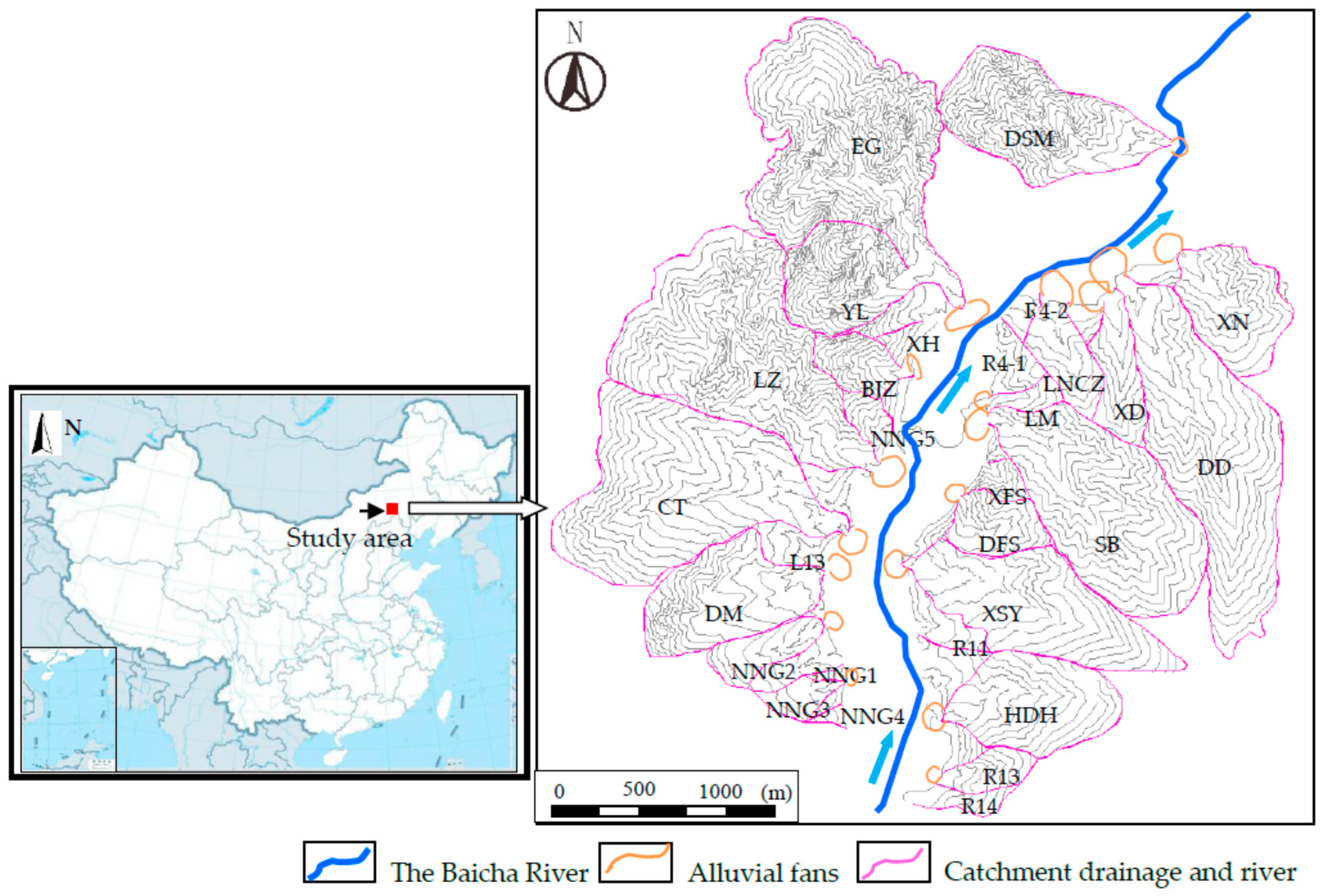
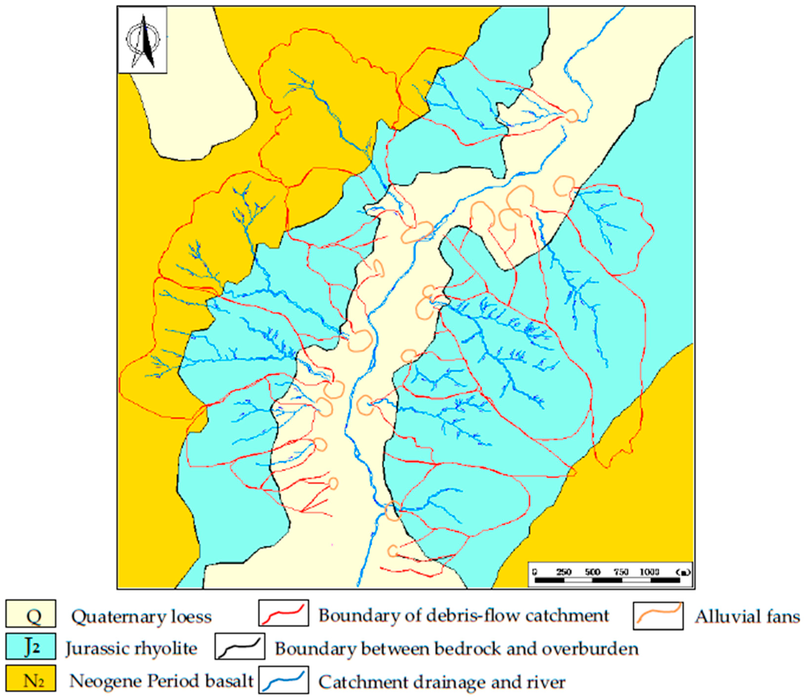
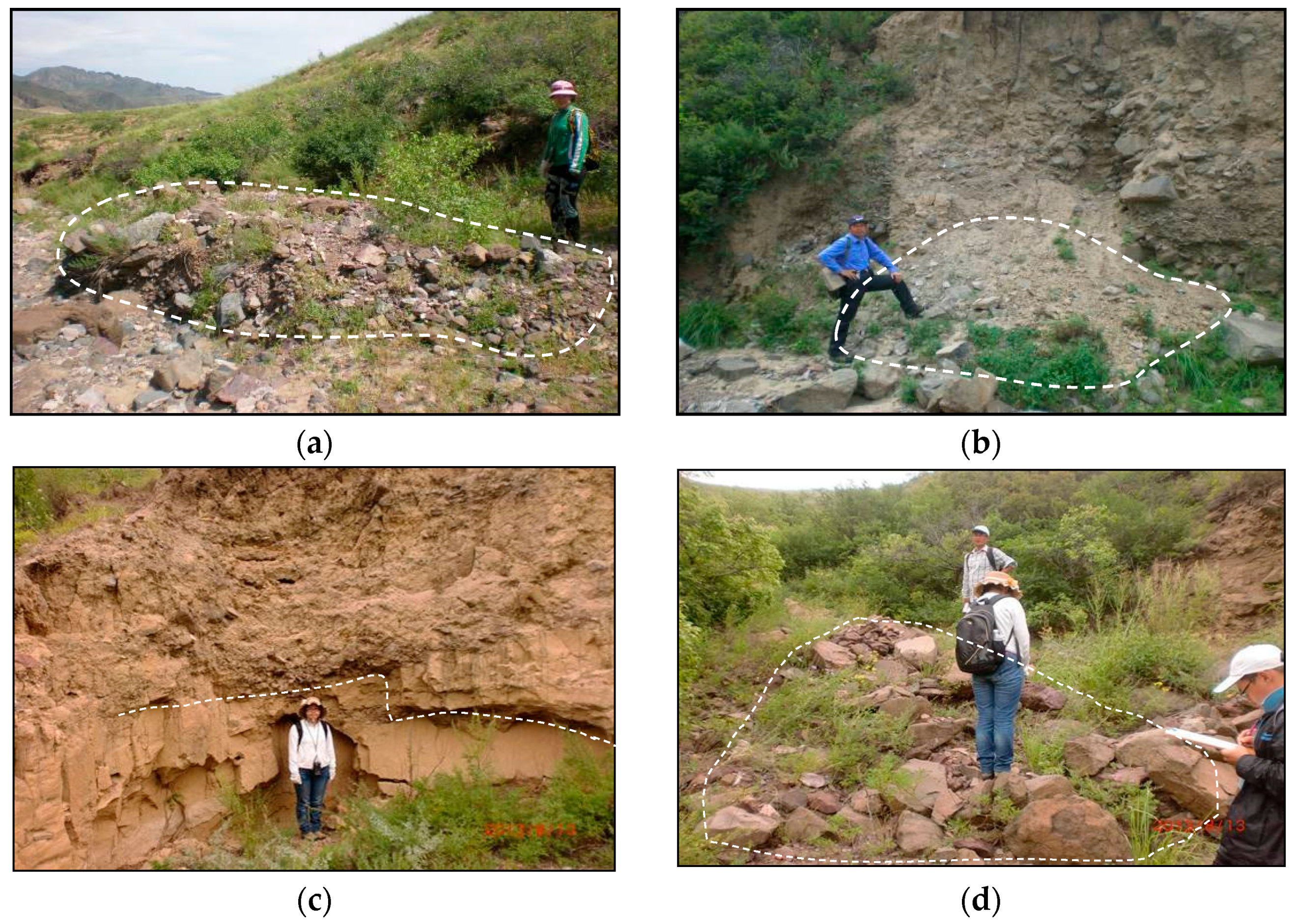
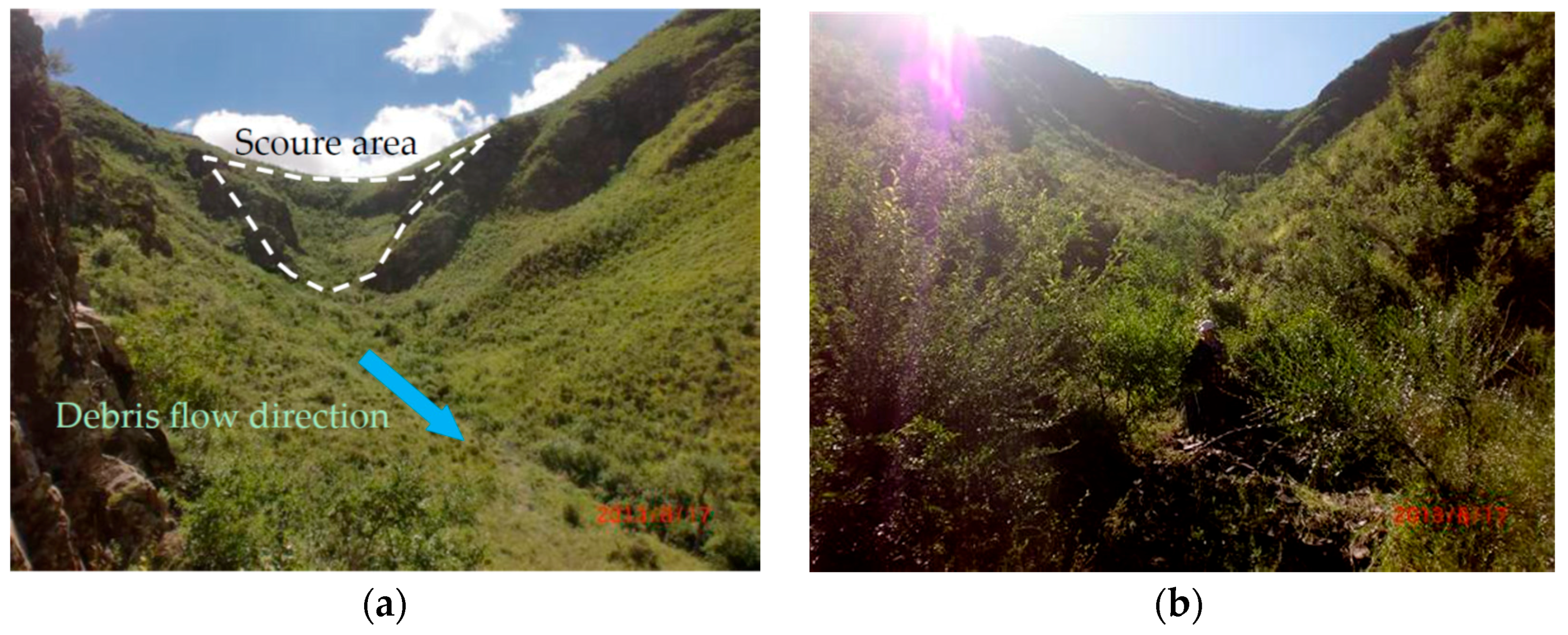
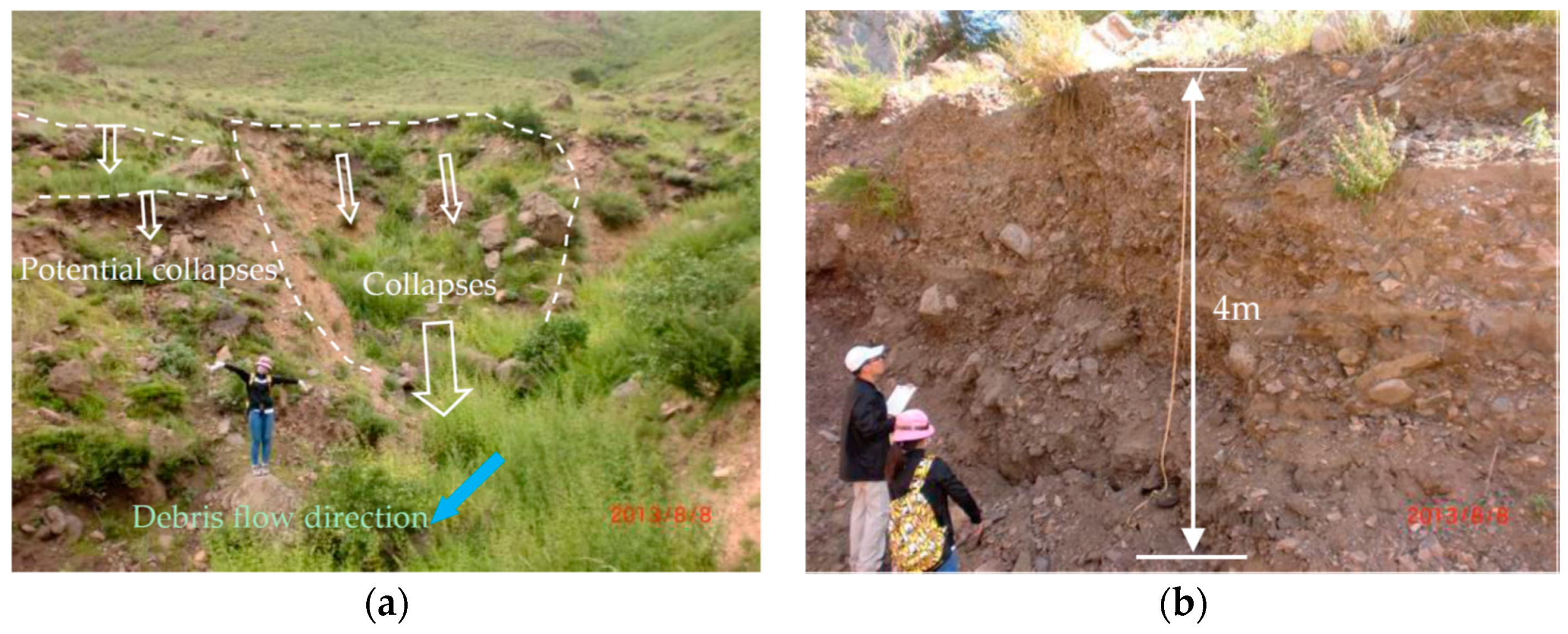
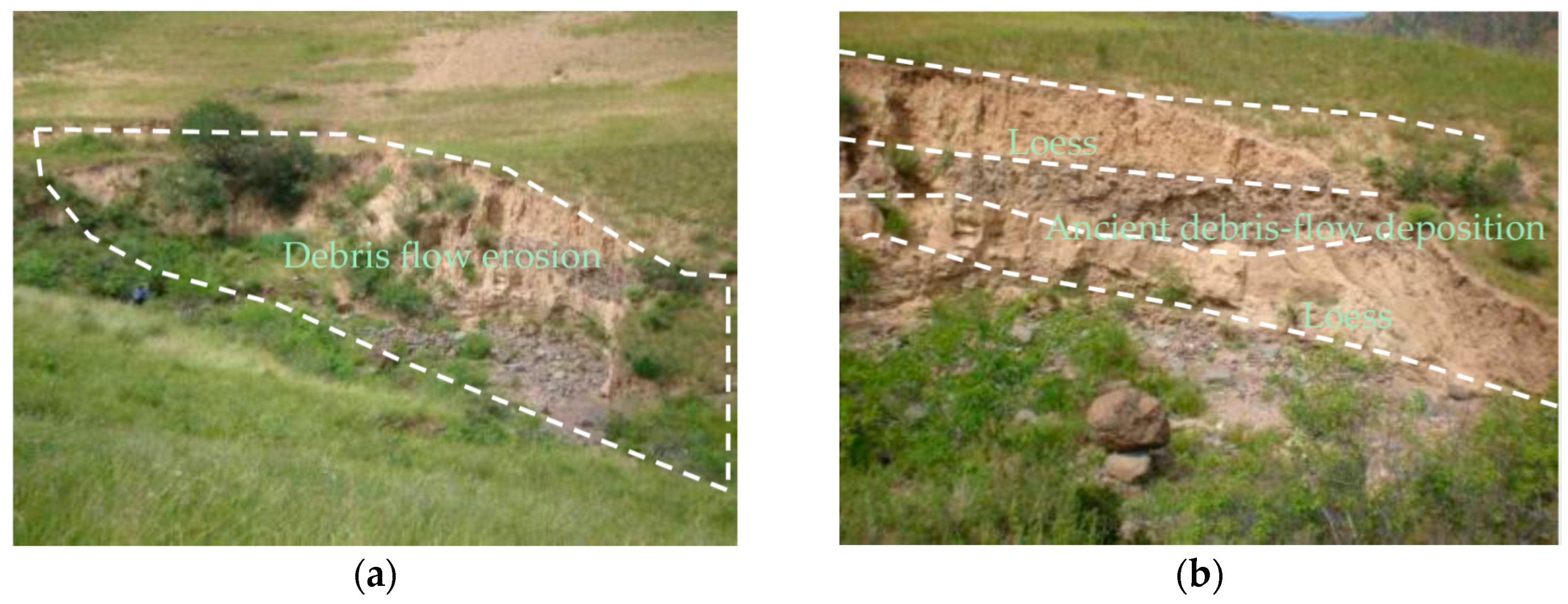
2. Study Area

The study area of the pumped storage power station is located 3 km north of the town of Zhirui in Heshigten Banner, Inner Mongolia, China. The Baicha River flows from the SSW to the NNE through the lower reservoir before reaching Gaojiayingzi town. As shown in Figure 1, there are 29 DF catchments distributed along both banks of the Baicha River. Loose material is prone to discharge from the DF catchments, accumulating on the banks or cascading into the Baicha River itself. Therefore, it was considered necessary to conduct a hazard assessment of the DFs.

The elevation of this area ranges from 1100 to 1700 m above sea level. It lies within a middle-mountain district and the trend of the mountains is NE. Neogene basalts covering the surface of the mountains has led to the tops of the mountains to be shaped as flat terraces. The slope angles of the mountains range from 30° to 50°. The Baicha River is U-shaped and the width of the bed ranges from 200 to 500 m above sea level. There are three main types of exposed strata including Quaternary (Q) loess, Neogene (N₂) basalt, and Jurassic (J₂) rhyolite. The loess, basalt, and rhyolite are distributed around the Baicha River, as shown in Figure 2. No regional faulting is found within the study area. We used the global positioning system (GPS) to locate the field phenomenon, such as loose deposits, collapsed mass, and loose gravel distributed within the 29 DF catchments. Lateral erosion occurs via hydrodynamic scouring (Figure 3).

The study area is characterized by a temperate continental monsoon climate. The southern part is a warm–cool semiarid agroclimatic zone. The temperature in January is −24–−19 °C, and in July it is 17–21 °C. The northern part is a warm–cold wet semi forested climatic zone. The average annual temperature is 2–5 °C. The minimum and maximum temperatures are −18 and 21 °C, respectively. Annual rainfall in Heshigten Banner is 250–540 mm. In the forested areas of Dajuzi District, the annual average rainfall can reach 531.8 mm (maximum rainfall was 741.6 mm in 1959). In the pastoral areas, the annual average rainfall is 350–400 mm. The annual rainfall in the agricultural areas increases from east to west with most districts receiving 300–390 mm.

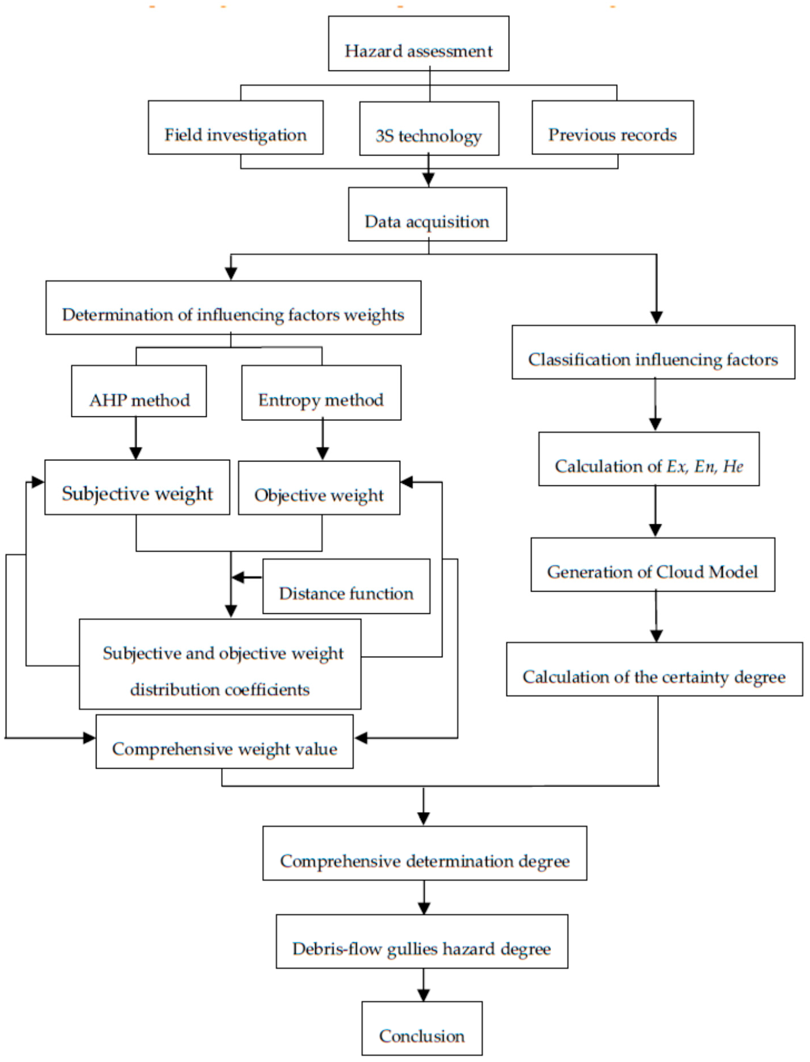
3. Methodology

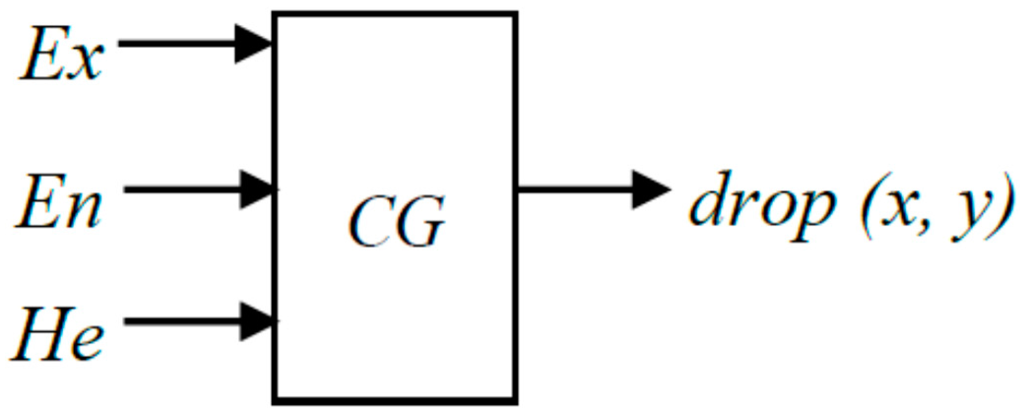
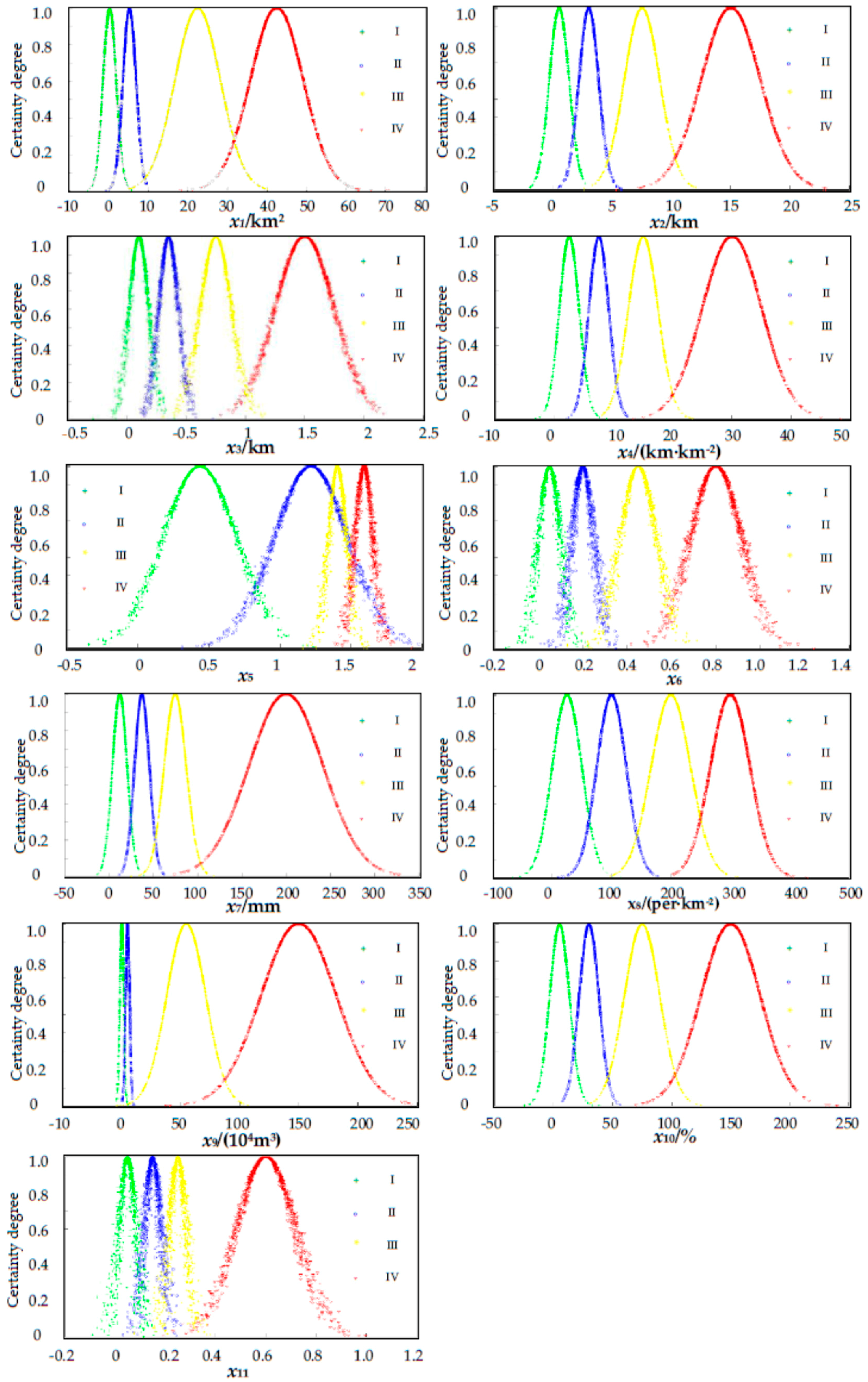
3.1. Cloud Model

Li [21] proposed a cloud model (CM), which is a conversion model between qualitative and quantitative numerical data. Based on probability theory and fuzzy mathematics, the CM explores the relationship between fuzziness and randomness. The CM is defined as follows. It is supposed that A is a quantitative domain expressed by accurate numbers and C is a quality concept in A. There exists a matching certainty degree μ(x) ∈ [0, 1] to C for arbitrary x∈A. The distribution of x in A is called a cloud and each x is called a cloud drop:

$$\mu : A\to [0, 1], \forall x\in A, x\to \mu \left(x\right)$$

(1)

A CM can be characterized by three quantitative characteristics [21,22]: expectation (E_x), entropy (E_n), and hyper-entropy (H_e). E_x is the mathematical expectation that a cloud drop belongs to a concept in the universal. It can be regarded as the most representative and typical sample of the qualitative concept. E_n represents the uncertainty measurement of a qualitative concept, the larger its value, the greater the fuzziness and randomness of the concept. It not only reflects the dispersing extent of cloud drops, but also the measurement of fuzziness. H_e is a measure of the randomness and fuzziness of E_n, which reflects the uncertainty aggregation degree of the cloud drop. Its value indirectly reflects the thickness of the cloud and is determined by randomness and fuzziness of entropy. The larger the value of H_e, the larger the randomness of the membership degree and the thickness of the cloud drops [23].

A cloud generator establishes a relationship between the qualitative and the quantitative characteristics. The cloud generator mainly includes a forward cloud generator and a backward cloud generator. The forward cloud generator is a basic cloud generator algorithm, which realizes the mapping of qualitative to quantitative characteristics. The input is the quantitative characteristics of the cloud (E_x, E_n, H_e) and cloud drops N. The output is the quantitative locations of the N cloud drops in the cloud and the certainty degree represented by each cloud drop, as shown in Figure 4.

The specific algorithm is as follows:

• Generate a normally distributed random number y_i, whose mean value is E_n and standard deviation is H_e.
• Generate a normally distributed random number x_i, whose mean value is E_x and standard deviation is y_i.
• Let x_i be a specific quantitative value of qualitative characteristics, named a cloud drop.
• Calculate the certainty degree of the random number: $\mu =e^{\frac{-{\left(x_i-E_x\right)}^2}{2y_i{}^2}}$.
• Output a cloud drop (x_i, μ_i).
• Repeat steps 1–5 until N cloud drops are generated and all the cloud drops comprise the cloud and realize a qualitative presentation.

3.2. Weighting Methods

(1) The analytical hierarchy process (AHP) is a multi-objective decision analysis method proposed by Saaty [24]. The weights of these criteria are defined after they are ranked according to their relative importance. Thus, once all the criteria are sorted in a hierarchical manner, a pairwise comparison matrix for each criterion is created to enable a significance comparison. The relative significances of the criteria are evaluated on a scale of 1–9, indicating less importance to greater importance. The steps of the AHP for weighting are as follows:

• The first step is to build the hierarchical structure of the target problem.
• Saaty [24] proposed a scaling method to score the parameters in each layer. By comparing the importance of the parameters in each level, a_ij is used to present the ratio of x_i and x_j, which builds the judgment matrix A = (a_ij):

  $$A={\left(a_{ij}\right)}_{n\times n}=\left[\begin{array}{cc}\begin{array}{cc}{a}_{11}& a_{12}\\ a_{21}& a_{22}\end{array}& \begin{array}{cc}\cdots & a_{1n}\\ \cdots & a_{2n}\end{array}\\ \begin{array}{cc}\cdots & \cdots \\ a_{n1}& a_{n2}\end{array}& \begin{array}{cc}\cdots & \cdots \\ \cdots & a_{nn}\end{array}\end{array}\right]$$

  (2)
• The judgment matrix needs to satisfy the following equation: 𝐴𝜔 = 𝜆_max𝜔, where ω is the maximum characteristic vector matching the feature vector of judgment matrix A. The weight value can be obtained after normalizing the feature vector.
• In order to analyze whether the weighting distribution is reasonable, a consistency check is needed. The consistency parameter (CI) can be obtained using the following equation:

  $$CI=\frac{{\lambda }_{\max }-n}{n-1}$$

  (3)

The random consistency ratio can be obtained using the following equation:

$$CR=CI/RI$$

(4)

where n is the order of the random index (RI). The value of RI can be obtained from Zhang [4]. If CR is lower than the threshold (0.1), the weighting consistency is affirmed, which means the weighting of the parameters is reasonable.

(2) The entropy method [25] is an objective weighting method that determines the weights of the parameters based on measured values. In information theory, entropy is a measure of the uncertainty of the formulation in terms of probability theory; greater amounts of information mean smaller degrees of uncertainty and entropy, and vice versa. According to the characteristics of entropy, the randomness and degree of disorder can be represented by the value of entropy. The discrete degree of a parameter is represented by its entropy value. The greater the discrete degree is, the larger the influence of the parameter on the comprehensive evaluation. If it is assumed there are m proposals to be assessed and n evaluation parameters, an original data matrix X = (x_ij)_m×n can be formed. For parameter x_j, the greater the parameter value X_ij, the more important the role that parameter plays in the comprehensive evaluation. If the values of an evaluation parameter are all equal, then that parameter does not play a role in the comprehensive evaluation. The occurrence of a DF is influenced by many parameters. It is difficult to describe DF hazard assessment using a traditional objective weighting method. However, the entropy theory can be used to assess the DF hazard. In this way, the disorder degree of the DF is expressed and given objective weights based on objective measured data. The steps of the weighting calculation using the entropy method are as follows:

• Standardize the data. After standardizing the original data matrix X = (x_ij)_m×n, obtain the normalized matrix R = (r_ij)_m×n. The normalizing equations are:
  The greater the better:

  $$r_{ij}=\frac{X_{ij}-\min \left\{X_{ij}\right\}}{\max \left\{X_{ij}\right\}-\min \left\{X_{ij}\right\}},\left(i=1,2,\dots ,n;j=1,2,\dots ,m\right)$$

  (5)
  The smaller the better:

  $$r_{ij}=\frac{\max \left\{X_{ij}\right\}-X_{ij}}{\max \left\{X_{ij}\right\}-\min \left\{X_{ij}\right\}},\left(i=1,2,\dots ,n;j=1,2,\dots ,m\right)$$

  (6)
• Calculate the i-th catchment j-th factor proportion:

  $$P_{ij}=\frac{X_{ij}}{{\displaystyle {\displaystyle \sum }_{i=1}^n}{X}_{ij}}\left(j=1,2,\dots ,m\right)$$

  (7)
• Calculate the information entropy of the factor:

  $$e_j=-k{\displaystyle \sum }_{i=1}^n{Y}_{ij}\times \ln Y_{ij}$$

  (8)

  where k > 0, ln is the natural logarithm, e_j ≥ 0, k is relative to the DF catchment number m, k = 1/lnm, and 0 ≤ e ≤ 1.
• Calculate the information entropy redundancy:

  $$g_j=1-e_j$$

  (9)
  As for the j-th factor, the greater the difference of the factor value X_ij, the greater the role that factor plays and the smaller the entropy value e_j.
• Calculate the factor weights:

  $$W_j=\frac{g_j}{{\displaystyle {\displaystyle \sum }_{j=1}^m}{g}_j},\left(i=1,2,\dots ,m\right)$$

  (10)

(3) The determination of the AHP judgment matrix is based on expert knowledge and the weighting of the entropy method depends on objective data. The objective and subjective weighting methods are combined into the EAHP weighting method using the distance function.

If it is assumed the weighting acquired by AHP is ${\omega }_i^{,}$ and the weighting calculated by the entropy method is ${\omega }_i^{,,}$, then the distance function of the two methods is d (${\omega }_i^{,}$, ${\omega }_i^{,,}$), whose equation is as follows:

$$d\left({\omega }_i^{,},{\omega }_i^{,,}\right)={\left[\frac{1}{2}{\displaystyle \sum }_{i=1}^n{({\omega }_i^{,}-{\omega }_i^{,,})}^2\right]}^{\frac{1}{2}}$$

(11)

Assume the combined weighting is ${\omega }_{\mathrm{z}}$, which is a linear weighting of ${\omega }_i^{,}$ and ${\omega }_i^{,,}$:

$${\omega }_{\mathrm{z}}=\alpha {\omega }_i^{,}+\beta {\omega }_i^{,,}$$

(12)

where α and β are two types of weighting partition coefficient.

In order to get the partition coefficients, the distance function is used, the equations for which are:

$$d\left({\omega }_i^{,},{\omega }_i^{,,}\right)={\left(\alpha -\beta \right)}^2$$

(13)

$$\alpha +\beta =1$$

(14)

The partition coefficients are obtained using Equations (13) and (14) and then substituted into Equation (12) to obtain the comprehensive weighting.

4. Debris-Flow Hazard Assessment

4.1. Evaluation Parameters

Previous research of DF hazard assessment has largely considered influencing parameters in terms of only four aspects: topography, meteorological and hydrological setting, geological setting, and anthropogenic activity. However, many other parameters influence DFs; therefore, it is necessary to include an appropriate selection for an accurate hazard assessment. Based on the principles of parameter selection for DF hazard assessment and other relevant studies [4,8,15,16,26,27,28,29,30,31,32,33,34,35,36,37,38], this study selected 11 influencing parameters based on the characteristics of the study area, as described below:

1. Catchment area (x₁/km²)

The catchment area reflects the confluence of the DF catchment and it represents the potential scale of the DF. However, it does not mean that larger catchment areas have greater hazard to DFs. Catchments of more than 100 km² appear susceptible to flooding. Here, catchment area was selected as an appropriate parameter, and the threshold was set as 0–50 km². Given that most of the 29 DF catchments within the study area are <0.5 km², the low hazard range was set as 0.0–0.5 km².

2. Main channel length (x₂/km)

The main channel length is the total length of the DF source and transportation areas. Long main channel lengths lead to larger-scale DFs with greater destructive power. Chang [16,20,39] regarded this as a very important parameter in terms of degree of risk, vulnerability to DFs, and hazard assessment. The scheme of Liu [40] was used for the classification of the degree of this parameter.

3. Maximum elevation difference (x₃/km)

This represents the difference between the maximum and minimum elevations of the catchment above sea level. It reflects the ability of the DF to carry solid material and provides an assessment of the catchment’s potential energy. In China, mountains are divided into four types based on elevation difference: <0.2 km are hills, 0.2–0.5 km are middle–low mountains, 0.5–1.0 km are high mountains, and >1.0 km are extremely high mountains.

4. Ravine density (x₄/km·km⁻²)

Ravine density is the ratio of the total ravine length to the total catchment area. The ravine reflects the geological structure, lithology, and the degree of rock weathering comprehensively because ravines always develop in weak areas [8]. The range of lateral erosions and retrogressive are reflected by ravine. With the development of the debris flows, the ravine density would gradually increase. Generally, higher ravine density corresponds to higher cumulative debris volume.

5. Curvature of the main channel (x₅)

According to previous studies [41,42,43], x₅ reflects the discharge situation of a DF. It represents the ratio of the curve length of the main channel to a straight length joining the same two measurement points. Erosion by water has an impact on the stability of slopes. If slope failure happens, the supply of loose material to the channel will be increased [44]. Here, the classification method of Liu [40] was used for this parameter.

6. Loose material length supply ratio (x₆)

This factor is defined as the ratio of loose material length along a channel to total channel length. It reflects the supply range and volume of loose material comprehensively. A higher x₆ value results in a wider range of loose the materials, which could make more debris volume added in the debris flow. Thus, the higher the x₆ value is, the higher the threat of debris flow. It directly influences the DF scale, which has a close relationship with DF hazard assessment. The number of possible slope phenomena and potential volumes of mobilized material from source areas to the main river [37]. Previous work suggests that a supply ratio of <0.1 indicates a catchment with no DF hazard, 0.1–0.3 is slightly hazardous, 0.3–0.6 is moderately hazardous, and >0.6 is highly hazardous [40].

7. Twenty-four-hour maximum rainfall (x₇/mm)

Water is a vital component of a DF because it is the transport medium. In the study area, rainfall is the only source of water and it is one of the main parameters that induce DFs [39,45]. Debris flows are mainly triggered by heavy rains [38]. The assessment of debris flow relies mainly on rain intensity [29].

8. Population density (x₈/per·km⁻²)

Anthropogenic activities have a close relationship with DFs and many DFs have been triggered by the negative consequences of socioeconomic development. Human activity, such as deforestation and slope cutting, accelerates the formation and development of debris flows seriously [8]. Landslides and slag caused by constructing roads and mining will increase the amount of loose material, thus increases the hazardous of debris flow. This parameter represents the strength of anthropogenic activities.

9. Loose material volume (x₉/10⁴ m³)

The abundance of loose material is a necessary condition that determines the scale of DFs [5,36]. Catchments with steep mountains experience large sediment pulses from hillslopes which are stored in headwater channels [35]. Within the catchments, this parameter was assessed using measurement and a laser rangefinder.

10. Outbreak frequency (x₁₀/%)

Even on a small scale, if the DF outbreak frequency is high, it could still cause considerable harm to the population and severe damage to properties within the catchment. Outbreak frequency represents the occurrence of DFs per 100 years. Considering the actual conditions of China, this study set the highest degree as once per year and the lowest degree as once every 10 years.

11. Main channel gradient (x₁₁)

Previous studies have shown that the average gradient of the main channel has a close relationship with the triggering of DFs [39,41,45,46,47,48,49]. Higher gradients imply greater DF velocity and greater energy for destruction. The main channel gradients in this study were obtained using field survey data and geographic information system technology. The classification scheme was largely based on Zhang [4].

The corresponding flow chart of the process is shown in Figure 5.

4.2. Establishment of the Cloud Model

Based on the above, a CM was used to establish a DF hazard assessment model. Following CM theory, the quantitative characteristics (E_x, E_n, H_e) were calculated using the following equations:

$$E_x^p=\frac{M_p+N_p}{2}p\left(p= 1,2,\dots ,P\right)$$

(15)

$$E_n^p=\{\begin{array}{c}\frac{E_x^2-E_x^1}{3}p=1\\ \frac{E_x^p-E_x^{p-1}}{3}p\ge 2\end{array}p\left(p= 1,2,\dots ,P\right)$$

(16)

$$H_e=\beta$$

(17)

where p is the hazard degree of the DF catchment, M_p and N_p are the upper boundary and lower boundary of a certain evaluation parameter of the i-th degree, and β is a constant. The value of H_e indirectly reflects the thickness of the cloud. In order to obtain accuracy certainties, β was set as 0.01 in this study. The boundaries are shown in

Table 1. Classification of influencing parameters.

Parameters	I	II	III	IV
x1 (km2)	0–0.5	0.5–10	10–35	35–50
x2 (km)	0–1	1–5	5–10	10–20
x3 (km)	0–0.2	0.2–0.5	0.5–1.0	1.0–2.0
x4 (km·km−2)	0–5	5–10	10–20	20–40
x5	0–1.10	1.10–1.25	1.25–1.40	1.40–1.55
x6	0–0.1	0.1–0.3	0.3–0.6	0.6–1.0
x7 (mm)	0–25	25–50	50–100	100–300
x8 (per·km−2)	0–50	50–150	150–250	250–350
x9 (104 m3)	0–1	1–10	10–100	100–200
x10 (%)	0–10	10–50	50–100	100–200
x11	0–0.1	0.1–0.2	0.2–0.35	0.35–0.85

x₁: catchment area; x₂: main channel length; x₃: maximum elevation difference; x₄: ravine density; x₅: curvature of main channel; x₆: loose material supply length ratio; x₇: twenty-four-hour maximum rainfall; x₈: population density; x₉: loose material volume; x₁₀: outbreak frequency; x₁₁: main channel gradient. I: low, II: moderate, III: high, and IV: extremely high.

.

The forward cloud generator was applied to generate clouds with the quantitative characteristics. The clouds, which are represented as low (I), moderate (II), high (III), and extremely high (IV), are shown in Figure 6. The CM has the ability for qualitative and quantitative transformation to determine the hazard degree for each parameter. Furthermore, the CM-based approach also considers the fuzziness and randomness of each parameter in adjacent degrees.

Table 2. Influencing parameter data of 29 debris-flow catchments.

Catchment	x1	x2	x3	x4	x5	x6	x7	x8	x9	x10	x11
DSM	0.667	1.276	0.445	1.927	1.226	0.55	251.8	0.1	0.608	1.06	0.35
EG	1.803	2.119	0.423	3.566	1.072	0.15	251.8	0.1	3.276	0.93	0.26
XH	0.034	0.249	0.159	12.44	1.073	0.38	251.8	0.1	0.044	0.97	0.36
BJZ	0.143	0.326	0.092	2.28	1.02	0.4	251.8	0.1	0.092	1.06	0.27
NN5	0.069	0.281	0.088	6.493	1.156	0.56	251.8	0.1	0.104	0.95	0.32
LZ	1.313	2.051	0.391	4.726	1.222	0.6	251.8	0.1	0.77	1.11	0.24
CT	1.302	2.051	0.4	4.51	1.145	0.6	251.8	0.1	3.995	2.90	0.27
DM	0.5525	0.856	0.098	2.77	1.07	0.3	251.8	0.1	0.7	1.07	0.32
NNG2	0.161	0.67	0.139	7.66	1.098	0.2	251.8	0.1	0.193	1.12	0.19
NNG1	0.06	0.334	0.057	11.75	1.034	0.2	251.8	0.1	0.055	1.05	0.19
NNG3	0.052	0.331	0.061	13.423	1.078	0.08	251.8	0.1	0.058	1.09	0.23
NNG4	0.021	0.187	0.057	10.667	1.022	0.08	251.8	0.1	0.0001	1.00	0.34
L13	0.099	0.387	0.064	5.21	1.06	0.3	251.8	0.1	0.006	1.00	0.19
XN	0.408	0.858	0.215	6.3	1.007	0.4	251.8	0.1	0.393	0.89	0.21
DD	1.598	2.591	0.463	3.992	1.328	0.4	251.8	0.1	6.513	3.56	0.19
XD	0.211	0.977	0.233	6.93	1.132	0.61	251.8	0.1	1.452	0.64	0.21
LNCZ	0.154	0.697	0.129	7.08	1.057	0.2	251.8	0.1	0.217	0.81	0.16
R4-1	0.028	0.196	0.097	16.1	1.021	1.0	251.8	0.1	0.0001	1.00	0.14
R4-2	0.013	0.26	0.1	20	1.066	1.0	251.8	0.1	0.0001	1.00	0.18
R5	0.038	0.226	0.087	11.63	1.092	0.45	251.8	0.1	0.085	0.45	0.27
LM	0.069	0.393	0.131	9.975	1.251	0.35	251.8	0.1	0.19	0.76	0.42
SB	1.082	1.664	0.355	5.21	1.074	0.4	251.8	0.1	3.38	0.46	0.18
XFS	0.064	0.247	0.16	7.78	1.025	0.25	251.8	0.1	0.307	0.62	0.37
DFS	0.197	0.633	0.203	7.761	1.347	0.31	251.8	0.1	0.605	0.50	0.18
XSY	0.755	1.565	0.258	3.91	1.059	0.53	251.8	0.1	3.244	0.53	0.18
R11	0.1142	0.37	0.161	3.616	1.09	0.25	251.8	0.1	0.154	0.83	0.31
HDH	0.516	1.25	0.245	4.73	1.136	0.35	251.8	0.1	1.732	0.61	0.14
R13	0.078	0.472	0.16	11.22	1.103	0.006	251.8	0.1	0.424	0.83	0.32
R14	0.058	0.291	0.155	17.5	1.111	0.35	251.8	0.1	0.146	0.66	0.31

is the basic data that obtained through field investigation and 3S technologies. The three-dimensional (3-D) characteristics of the 29 DF catchments were obtained through a digital elevation model (DEM), which is constructed to obtain factors related to elevation. Meanwhile, the catchment area is also obtained through GIS software.

4.3. Calculation of Weights Using the EAHP Method

Considering that different evaluation parameters have different contributions to DF hazard, it is important to develop an appropriate weighting method for the assessment. To begin, the AHP weighting method can be used to calculate subjective weights. By arbitrarily comparing pairs of parameters, it is possible to determine the relative importance of the 11 parameters. The basic geological data (Table 2) of the 29 DF catchments were applied to calculate the objective weights using the entropy method. Because of the shortcomings of using objective weighting method or subjective weighting method alone, it is necessary to combine the AHP and the entropy method. The combined weights were calculated using Equations (12)–(14).

4.4. Hazard Assessment of Debris-Flow

The CM certainty degree of X_ij is calculated based on the forward cloud generator. Meanwhile, the comprehensive certainty degree should be calculated using the following equation:

$$\begin{array}{l}{U}_{i,p}={\displaystyle {\displaystyle \sum }_{j=1}^m}{\mu }_{i,pj}{w}_j\\ i\left(i =1,2,\dots ,n\right);j\left(j= 1,2,\dots ,m\right);p\left(p= 1,2,\dots ,P\right)\end{array}$$

(18)

where μ_i,pj is the p-th hazard degree matching the certainty degree of the j-th factor of the i-th catchment and w_j is the evaluation factor weight of the DF. According to the comprehensive certainty degree U_p,i, it can be determined that the largest comprehensive certainty degree is the hazard degree of the matching DF catchment:

$$k= max\{U_{i,}{}_1,U_{i,}{}_2,\dots ,U_{p,n}\}$$

(19)

After precise calculation, the certainty values of the 11 parameters of the 29 DF catchments were obtained. The comprehensive certainty was obtained based on Equation (18). The largest comprehensive certainty value matching the hazard degree is the DF catchment hazard degree.

5. Results and Discussion

Based on the judgment matrix, CI was calculated based on λ_max = 11.30, n = 11, and RI = 1.52; thus, the value of CR = 0.0195 was calculated. As the value of CR is lower than the threshold (0.1), the consistency of the weighting was affirmed. The AHP weighting results are shown in

Table 3. Weights of influencing parameters in different methods.

Method	x1	x2	x3	x4	x5	x6	x7	x8	x9	x10	x11
AHP	0.132	0.053	0.085	0.037	0.017	0.062	0.105	0.017	0.18	0.18	0.132
Entropy	0.287	0.132	0.078	0.069	0.001	0.076	0	0	0.323	0.015	0.019
Combined	0.178	0.076	0.083	0.046	0.012	0.066	0.073	0.012	0.223	0.13	0.098

. There is only one rainfall monitoring station within the study area, and hence the same rainfall data were used for all the catchments. Furthermore, the location of the study area is remote and few people live here. Because of the characteristics of the entropy method, the weights of the 24-h maximum rainfall and population density were both zero, which means there is no difference between these two parameters in terms of the hazard degree. However, rainfall is one of the most important parameters in DF hazard assessment. This is an example of how the entropy method just reflects the objective results of the investigation and does not reflect expert knowledge. The coefficients are calculated as α = 0.695 and β = 0.305. The entropy weights and combined weights are shown in Table 3.

An evaluation system for DF hazard assessment, based on a CM that included 11 parameters, has been proposed. The hazard degrees of 29 catchments within the study area and their comparison with the extenics method are listed in

Table 4. Evaluation results of cloud model and comparison.

CCD	k1	k2	k3	k4	Cloud Model	Extenics
DSM	0.573	0.074	0.067	0.110	Low	Low
EG	0.277	0.384	0.079	0.074	Moderate	Low
XH	0.624	0.111	0.053	0.080	Low	Low
BJZ	0.504	0.152	0.115	0.048	Low	Low
L5	0.652	0.156	0.032	0.083	Low	Low
LZ	0.478	0.168	0.106	0.093	Low	Low
CT	0.306	0.363	0.120	0.093	Moderate	Moderate
DM	0.443	0.146	0.057	0.103	Low	Low
NNG2	0.346	0.172	0.072	0.072	Low	Low
NNG1	0.468	0.116	0.035	0.013	Low	Low
NNG3	0.504	0.164	0.011	0.085	Low	Low
NNG4	0.382	0.090	0.031	0.017	Low	Low
L13	0.425	0.110	0.077	0.082	Low	Low
XN	0.463	0.117	0.130	0.073	Low	Low
DD	0.153	0.179	0.218	0.089	High	High
XD	0.461	0.136	0.042	0.076	Low	Low
LNCZ	0.329	0.101	0.036	0.076	Low	Low
R4-1	0.442	0.037	0.053	0.015	Low	Low
R4-2	0.503	0.102	0.098	0.073	Low	Low
R5	0.333	0.086	0.074	0.014	Low	Low
LM	0.533	0.099	0.085	0.027	Low	Low
SB	0.292	0.396	0.075	0.072	Moderate	Moderate
XFS	0.304	0.186	0.096	0.077	Low	Moderate
DFS	0.427	0.096	0.113	0.030	Low	Low
XSY	0.306	0.113	0.077	0.071	Low	Low
R11	0.395	0.104	0.142	0.070	Low	Low
HDH	0.452	0.218	0.099	0.063	Low	Low
R13	0.425	0.046	0.030	0.041	Low	Low
R14	0.393	0.086	0.056	0.020	Low	Low

Note: CCD is the comprehensive certainty degree.

. Among the 29 catchments, the hazard degree of catchment DD is high, that of catchments EG, CT, and SB is moderate, and that of the remaining catchments is low. Note that the area of each of the 29 catchments is very small, ranging from 0.013 to 1.803 km². Field surveys showed that no large-scale collapses or landslides existed and that rainfall was not abundant in northern China [50,51]. Thus, the study area was more prone to small-scale and medium-scale DFs [27].

As can be seen in Table 4, the hazard assessment results for the 29 DF catchments, calculated using the proposed approach, are reasonably consistent with the results of the extenics method. The extenics methodwas first proposed by Cai [52] to solve contradictions and incompatibility problems. It is based on matter-element theory and extension mathematics. It concerns not only whether an element belongs to a set but also concerns to what degree it belongs. Thus, it is representative of traditional comprehensive evaluation methods and it has been proven reliable and reasonable for classification [5,53,54,55,56]. In extension theory, h (x) is the correlation function, which represents the degree an element belongs to a set. If h (x) ≥ 0, it describes the degree to which the element belongs to the set. If −1 < h (x) < 0, it indicates that the element does not belong to the set. Nevertheless, the element still has a better chance to be included if the set varies. When h (x) ≤ −1, it means that the element has no chance to be included by the set. The value describes the degree of the element not belonging to the set [57,58]. The proposed method used for the hazard assessment was considered efficient and believable. The hazard assessment results derived using the two methods correlated very well, except for catchments EG and XFY, where the CM-based results were moderate and low, respectively. The evaluation accuracy was nearly 93.1%, which indicated that the CM-based approach had precise evaluation capability. The slight deviation was considered acceptable and understandable for a hazard assessment of the actual project.

Compared with the widely used extenics approach, the CM-based approach appeared to offer a more competitive solution for addressing the uncertainties [59]. However, expert knowledge based on field surveys was also a major aspect. As can be seen in Table 4, the results for catchments EG and XFY derived by the extenics method were low and moderate, respectively. They differed from the analyzed results of the CM-based approach because of inadequate objective data and because expert knowledge is very important in the DF hazard assessment. Many existing methods are vulnerable to the subjective and ambiguous in the process of assessment; however, the CM-based approach could overcome these disadvantages and provide an efficient assessment [60,61]. The determination of the parameter types and their boundaries depends mainly on expert knowledge, but human error does occur, which could affect the accuracy and reliability of the derived results. However, the CM-based approach reduces the deviation because it considers the inherent fuzziness and randomness of such problems. The CM-based approach can directly use the original data without a normalization procedure, effectively avoiding the potential information loss.

In the proposed approach, weights are assigned to the 11 parameters. The subjective weighting method is limited by the extent of expert knowledge, and different researchers have had different experiences and have used different evaluation criteria [45,62,63]. However, the objective weighting method depends on information that does not require expert knowledge. Obtaining sufficient data is laborious and expensive [59], and therefore the combination of the subjective and objective weighting methods was necessary [64]. However, the weights of the 11 parameters calculated based on the combination weighting method may be difficult to be evaluated due to the complexity of the modeling process. Thus, determination of the more accurate weights still needs unremitting efforts.

The EG is assessed as moderate hazardous degree using CM method, while the extenics result is low hazardous. On the right side of main channel in EG catchment, there exists a lot of collapses and potential collapses (Figure 7a). The collapsed mud and gravel has been washed along the debris flow in the main channel. Meanwhile, there is existing potential collapses in the neighborhood, which may collapse down induced by the next rainfall. There exists two fans in the EG accumulation area. One is an ancient alluvial fan, the other one is a younger alluvial fan. The younger one is shaped as ellipse, whose long axis is 373.5 m and short axis is 90 m. Figure 7b shows the profile of the younger alluvial fan, which is about 4 m thick. The loose material volume of EG is 3.276 × 10⁴ m³, which is very large among the 29 catchments. The hazardous of EG catchment should be moderate instead of low. The assessment result of XFS using the extenics method is moderate, while the result of XFS using CM is low. In the field, we didn’t find any landslides or collapses in the source area.

Figure 8 shows that the XFS catchment is well covered with vegetation. The vegetation cover greatly influence slope behavior at every scale [41]. XFS is a small catchment, with less volume of loose material. The hazardous degree of XFS catchment should be low. And the proposed CM is more believable. The CM-based hazard assessment result for catchment DD was high. Figure 9 shows a cross section that reveals that the left bank of the main channel in catchment DD has been subject to processes of erosion and collapse. In the profiles, gravel soil and loess appear alternately, both of which are about 2 m thick. The gravel soil layer is an ancient DF ditch bed. During periods in between DFs, loess was deposited on the surface. Then, a subsequent DF would cut the ancient DF ditch bed. Consequently, it can be inferred that DFs have occurred in the DD catchment at least three times. According to Table 2, the outbreak frequency of DD catchment is 3.56 times per 100a. Therefore, the three events occurred in 100 years. Therefore, the determination of the hazard assessment of the DD catchment as high was reasonable.

In the proposed approach, weights are assigned to the 11 parameters. The subjective weighting method is limited by the extent of expert knowledge, and different researchers have had different experiences and have used different evaluation criteria [45,62,63]. However, the objective weighting method depends on information that does not require expert knowledge. Obtaining sufficient data is laborious and expensive [59], and therefore the combination of the subjective and objective weighting methods was necessary [64]. However, the weights of the 11 parameters calculated based on the combination weighting method may be difficult to be evaluated due to the complexity of the modeling process. Thus, determination of the more accurate weights still needs unremitting efforts.

6. Conclusions

Because DFs constitute open, multi-parameter and complex problems, it is difficult to distinguish the randomness and fuzziness of each evaluation parameter. This study used a CM for DF hazard assessment because of the ease with which it can transform the qualitative and quantitative descriptions. According to the 11 selected parameters and their weights, a CM-based approach was established to classify the degree of hazard assessment of DF catchments. Compared with the extenics method, the CM-based hazard assessment approach was validated as credible with an evaluation accuracy of 93.1%. The CM-based approach was shown suitable for a DF hazard assessment, which is a problem of transforming qualitative and quantitative expressions. Furthermore, it considered the uncertainty of randomness and fuzziness in the assessment. The CM-based approach is a type of decision tool that could have wide application to other hazard assessment projects.

This study proposed a new combined weighting method using the distance function for deriving parameter weights, which avoids the disadvantages inherent in using the subjective and objective methods in isolation. The results were proven reasonably consistent with the actual situation.

After a detailed analysis of the original datasets and the proposed approach characteristics, it demonstrates its superiority and validity for the hazard assessment of DF. The results of CM-based approach are reasonable. However, the reliability evaluation result of the cloud model depends on the selection of boundaries of different degrees of an evaluation parameter. These parameters boundaries need expert’s field survey experiences and lots of research to obtain. The comprehensive assessment for DF hazard assessment, how to determine the relevant parameters boundaries more reasonably and accurately should be improved in the future.

The CM-based approach can adequately reflect the hazard degree of DF catchments in the study area Despites the above merits, the CM-based method has its disadvantages. The cloud model requires a lot of input, mainly including expect value (E_x), entropy (E_n), hyper-entropy (H_e) and the number of cloud drops (N). The inputs were determined by the classification boundaries of the debris flow hazard assessment, which does not have a verdict. A reasonable determination of the three characteristics of the model should be studied in the future. Since the CM-based approach is still in the phase of theory, it needs to be applied and validated for more study areas in the future.

References

- Jakob, M.; Hungr, O.; Jakob, D.M. Debris-Flow Hazards and Related Phenomena; Springer: Berlin, Germany, 2005. [Google Scholar]
- Giannecchini, R.; Naldini, D.; Avanzi, G.D.A.; Puccinelli, A. Modelling of the initiation of rainfall-induced debris flows in the Cardoso basin (Apuan Alps, Italy). Quat. Int. 2007, 171, 108–117. [Google Scholar] [CrossRef]
- De Scally, F.; Owens, I.; Louis, J. Controls on fan depositional processes in the schist ranges of the Southern Alps, New Zealand, and implications for debris-flow hazard assessment. Geomorphology 2010, 122, 99–116. [Google Scholar] [CrossRef]
- Zhang, W.; Chen, J.; Wang, Q.; An, Y.; Qian, X.; Xiang, L.; He, L. Susceptibility analysis of large-scale debris flows based on combination weighting and extension methods. Nat. Hazards 2013, 66, 1073–1100. [Google Scholar] [CrossRef]
- Niu, C.-C.; Wang, Q.; Chen, J.-P.; Wang, K.; Zhang, W.; Zhou, F.-J. Debris-flow hazard assessment based on stepwise discriminant analysis and extension theory. Q. J. Eng. Geol. Hydrogeol. 2014, 47, 211–222. [Google Scholar] [CrossRef]
- Ni, H.; Zheng, W.; Li, Z.; Ba, R. Recent catastrophic debris flows in Luding county, SW China: Geological hazards, rainfall analysis and dynamic characteristics. Nat. Hazards 2010, 55, 523–542. [Google Scholar] [CrossRef]
- Zhang, C.; Chen, J.-P.; Wang, Q.; Zhang, W. Study on debris flow based on fractal theory and characteristics of water system. Shuili Xuebao (J. Hydraul. Eng.) 2011, 42, 351–356. [Google Scholar]
- Zhang, W.; Li, H.; Chen, J.; Zhang, C.; Xu, L.; Sang, W. Comprehensive hazard assessment and protection of debris flows along Jinsha river close to the Wudongde dam site in China. Nat. Hazards 2011, 58, 459–477. [Google Scholar] [CrossRef]
- Eldeen, M.T. Predisaster physical planning: Integration of disaster risk analysis into physical planning–A case study in Tunisia. Disasters 1980, 4, 211–222. [Google Scholar] [CrossRef] [PubMed]
- Hollingsworth, R.; Kovacs, G. Soil slumps and debris flows: Prediction and protection. Bull. Assoc. Eng. Geol. 1981, 18, 17–28. [Google Scholar] [CrossRef]
- Özdemir, A.; Delikanli, M. A geotechnical investigation of the retrogressive Yaka landslide and the debris flow threatening the town of Yaka (Isparta, sw Turkey). Nat. Hazards 2009, 49, 113–136. [Google Scholar] [CrossRef]
- Chiou, I.J.; Chen, C.H.; Liu, W.L.; Huang, S.M.; Chang, Y.M. Methodology of disaster risk assessment for debris flows in a river basin. Stoch. Environ. Res. Risk A 2015, 29, 775–792. [Google Scholar] [CrossRef]
- Liu, H.; Tang, C. Development of digital disaster reduction system for debris flow in urban district of Dongchuan. J. Nat. Disasters 2007, 16, 7. [Google Scholar]
- Carrara, A.; Crosta, G.; Frattini, P. Comparing models of debris-flow susceptibility in the Alpine environment. Geomorphology 2008, 94, 353–378. [Google Scholar] [CrossRef]
- Liang, W.; Zhuang, D.; Jiang, D.; Pan, J.; Ren, H. Assessment of debris flow hazards using a bayesian network. Geomorphology 2012, 171, 94–100. [Google Scholar] [CrossRef]
- Chang, T.-C. Risk degree of debris flow applying neural networks. Nat. Hazards 2007, 42, 209–224. [Google Scholar] [CrossRef]
- Han, G.; Wang, D. Numerical modeling of Anhui debris flow. J. Hydraul. Eng. 1996, 122, 262–265. [Google Scholar] [CrossRef]
- Gomez, H.; Kavzoglu, T. Assessment of shallow landslide susceptibility using artificial neural networks in Jabonosa river basin, Venezuela. Eng. Geol. 2005, 78, 11–27. [Google Scholar] [CrossRef]
- Lin, G.-F.; Chen, L.-H.; Lai, J.-N. Assessment of risk due to debris flow events: A case study in central Taiwan. Nat. Hazards 2006, 39, 1–14. [Google Scholar] [CrossRef]
- Chang, T.-C.; Chien, Y.-H. The application of genetic algorithm in debris flows prediction. Environ. Geol. 2007, 53, 339–347. [Google Scholar] [CrossRef]
- Deyi, L.; Haijun, M.; Xuemei, S. Membership clouds and membership cloud generators. J. Comput. Res. Dev. 1995, 6, 15–20. [Google Scholar]
- Li, D.; Liu, C.; Gan, W. A new cognitive model: Cloud model. Int. J. Intell. Syst. 2009, 24, 357–375. [Google Scholar] [CrossRef]
- Chen, J.-F.; Zhao, S.-F.; Shao, Q.-X.; Wang, H.-M. Risk assessment on drought disaster in China based on integrative cloud model. Res. J. Appl. Sci. Eng. Technol. 2012, 4, 1137–1146. [Google Scholar]
- Saaty, T.L. How to make a decision: The analytic hierarchy process. Eur. J. Oper. Res. 1990, 48, 9–26. [Google Scholar] [CrossRef]
- Zeleny, M.; Cochrane, J.L. Multiple Criteria Decision Making; University of South Carolina Press: Columbia, SC, USA, 1973. [Google Scholar]
- Kuang, L.; Xu, L.; Liu, B. Debris flow hazard assessment based on extension method. China Railw. Sci. 2006, 5, 1–6. [Google Scholar]
- Niu, C.; Wang, Q.; Chen, J.; Zhang, W.; Xu, L.; Wang, K. Hazard assessment of debris flows in the reservoir region of wudongde hydropower station in China. Sustainability 2015, 7, 15099–15118. [Google Scholar] [CrossRef]
- Tiranti, D.; Cremonini, R.; Asprea, I.; Marco, F. Driving factors for torrential mass-movements occurrence in the Western Alps. Front. Earth Sci. 2016, 4, 16. [Google Scholar] [CrossRef]
- Nikolopoulos, E.; Borga, M.; Creutin, J.; Marra, F. Estimation of debris flow triggering rainfall: Influence of rain gauge density and interpolation methods. Geomorphology 2015, 243, 40–50. [Google Scholar] [CrossRef]
- Stoffel, M.; Tiranti, D.; Huggel, C. Climate change impacts on mass movements—Case studies from the European Alps. Sci. Total Environ. 2014, 493, 1255–1266. [Google Scholar] [CrossRef] [PubMed]
- Kean, J.W.; McCoy, S.W.; Tucker, G.E.; Staley, D.M.; Coe, J.A. Runoff-generated debris flows: Observations and modeling of surge initiation, magnitude, and frequency. J. Geophys. Res. Earth Surf. 2013, 118, 2190–2207. [Google Scholar] [CrossRef]
- Tiranti, D.; Deangeli, C. Modeling of debris flow depositional patterns according to the catchment and sediment source area characteristics. Front. Earth Sci. 2015, 3, 8. [Google Scholar] [CrossRef]
- Surian, N.; Righini, M.; Lucía, A.; Nardi, L.; Amponsah, W.; Benvenuti, M.; Borga, M.; Cavalli, M.; Comiti, F.; Marchi, L. Channel response to extreme floods: Insights on controlling factors from six mountain rivers in Northern Apennines, Italy. Geomorphology 2016, 272, 78–91. [Google Scholar] [CrossRef]
- Cavalli, M.; Trevisani, S.; Comiti, F.; Marchi, L. Geomorphometric assessment of spatial sediment connectivity in small alpine catchments. Geomorphology 2013, 188, 31–41. [Google Scholar] [CrossRef]
- Theule, J.; Liébault, F.; Loye, A.; Laigle, D.; Jaboyedoff, M. Sediment budget monitoring of debris-flow and bedload transport in the Manival Torrent, SE France. Nat. Hazards Earth Syst. Sci. 2012, 12, 731–749. [Google Scholar] [CrossRef]
- Guzzetti, F.; Ardizzone, F.; Cardinali, M.; Rossi, M.; Valigi, D. Landslide volumes and landslide mobilization rates in Umbria, central Italy. Earth Planet. Sci. Lett. 2009, 279, 222–229. [Google Scholar] [CrossRef]
- Tiranti, D.; Cavalli, M.; Crema, S.; Zerbato, M.; Graziadei, M.; Barbero, S.; Cremonini, R.; Silvestro, C.; Bodrato, G.; Tresso, F. Semi-quantitative method for the assessment of debris supply from slopes to river in ungauged catchments. Sci. Total Environ. 2016, 554, 337–348. [Google Scholar] [CrossRef] [PubMed]
- Tiranti, D.; Cremonini, R.; Marco, F.; Gaeta, A.R.; Barbero, S. The defense (debris flows triggered by storms–nowcasting system): An early warning system for torrential processes by radar storm tracking using a geographic information system (GIS). Comput. Geosci. 2014, 70, 96–109. [Google Scholar] [CrossRef]
- Chang, T.-C.; Chao, R.-J. Application of back-propagation networks in debris flow prediction. Eng. Geol. 2006, 85, 270–280. [Google Scholar] [CrossRef]
- Liu, X.; Tang, C. Debris Flow Hazardous Assessment; Science Press: Beijing, China, 1995. [Google Scholar]
- Catani, F.; Casagli, N.; Ermini, L.; Righini, G.; Menduni, G. Landslide hazard and risk mapping at catchment scale in the Arno river basin. Landslides 2005, 2, 329–342. [Google Scholar] [CrossRef]
- Lee, S.; Pradhan, B. Landslide hazard mapping at Selangor, Malaysia using frequency ratio and logistic regression models. Landslides 2007, 4, 33–41. [Google Scholar] [CrossRef]
- Tunusluoglu, M.; Gokceoglu, C.; Nefeslioglu, H.; Sonmez, H. Extraction of potential debris source areas by logistic regression technique: A case study from Barla, Besparmak and Kapi mountains (NW Taurids, Turkey). Environ. Geol. 2008, 54, 9–22. [Google Scholar] [CrossRef]
- Duo, T.; Wang, Y.; Huang, Z.; Duo, T. A fuzzy math evaluation on debris-flow occurrence in the three main gullies in Chayuangou Alley. J. Geol. Hazards Environ. Preserv. 2011, 22, 31–35. [Google Scholar]
- Tiranti, D.; Bonetto, S.; Mandrone, G. Quantitative basin characterisation to refine debris-flow triggering criteria and processes: An example from the Italian Western Alps. Landslides 2008, 5, 45–57. [Google Scholar] [CrossRef]
- Lin, P.-S.; Lin, J.Y.; Hung, J.-C.; Yang, M.-D. Assessing debris-flow hazard in a watershed in Taiwan. Eng. Geol. 2002, 66, 295–313. [Google Scholar] [CrossRef]
- Ohlmacher, G.C.; Davis, J.C. Using multiple logistic regression and GIS technology to predict landslide hazard in Northeast Kansas, USA. Eng. Geol. 2003, 69, 331–343. [Google Scholar] [CrossRef]
- Lan, H.; Zhou, C.; Wang, L.; Zhang, H.; Li, R. Landslide hazard spatial analysis and prediction using GIS in the Xiaojiang watershed, Yunnan, China. Eng. Geol. 2004, 76, 109–128. [Google Scholar] [CrossRef]
- Lu, G.Y.; Chiu, L.S.; Wong, D.W. Vulnerability assessment of rainfall-induced debris flows in Taiwan. Nat. Hazards 2007, 43, 223–244. [Google Scholar] [CrossRef]
- Liu, C.-N.; Dong, J.J.; Peng, Y.F.; Huang, H.-F. Effects of strong ground motion on the susceptibility of gully type debris flows. Eng. Geol. 2009, 104, 241–253. [Google Scholar] [CrossRef]
- Yu, B.; Zhu, Y.; Wang, T.; Chen, Y.; Zhu, Y.; Tie, Y.; Lu, K. A prediction model for debris flows triggered by a runoff-induced mechanism. Nat. Hazards 2014, 74, 1141–1161. [Google Scholar] [CrossRef]
- Cai, W. The extension set and incompatibility problem. J. Sci. Explor. 1983, 1, 81–93. [Google Scholar]
- Zheng, G.; Jing, Y.; Huang, H.; Zhang, X.; Gao, Y. Application of life cycle assessment (LCA) and extenics theory for building energy conservation assessment. Energy 2009, 34, 1870–1879. [Google Scholar] [CrossRef]
- Li, X.; Zhang, H.; Zhu, Z.; Xiang, Z.; Chen, Z.; Shi, Y. An intelligent transformation knowledge mining method based on extenics. J. Internet Technol. 2013, 14, 315–325. [Google Scholar]
- Wang, M.H.; Huang, M.L.; Liou, K.J. Application of extension theory with chaotic signal synchronization on detecting islanding effect of photovoltaic power system. Int. J. Photoenergy 2015, 2015, 1–10. [Google Scholar] [CrossRef]
- Zhao, B.; Xu, W.; Liang, G.; Meng, Y. Stability evaluation model for high rock slope based on element extension theory. Bull. Eng. Geol. Environ. 2015, 74, 301–314. [Google Scholar] [CrossRef]
- Wang, M.H.; Tseng, Y.F.; Chen, H.C.; Chao, K.H. A novel clustering algorithm based on the extension theory and genetic algorithm. Expert Syst. Appl. 2009, 36, 8269–8276. [Google Scholar] [CrossRef]
- Ye, J. Application of extension theory in misfire fault diagnosis of gasoline engines. Expert Syst. Appl. 2009, 36, 1217–1221. [Google Scholar] [CrossRef]
- Zhang, L.; Wu, X.; Chen, Q.; Skibniewski, M.J.; Zhong, J. Developing a cloud model based risk assessment methodology for tunnel-induced damage to existing pipelines. Stoch. Environ. Res. Risk A 2015, 29, 513–526. [Google Scholar] [CrossRef]
- Li, L.; Liu, L.; Yang, C.; Li, Z. The comprehensive evaluation of smart distribution grid based on cloud model. Energy Procedia 2012, 17, 96–102. [Google Scholar] [CrossRef]
- Sun, X.; Cai, C.; Yang, J.; Shen, X. Route assessment for unmanned aerial vehicle based on cloud model. Math. Probl. Eng. 2014, 2014, 1–13. [Google Scholar] [CrossRef]
- Wan, S.; Lei, T.; Huang, P.; Chou, T. The knowledge rules of debris flow event: A case study for investigation Chen Yu Lan River, Taiwan. Eng. Geol. 2008, 98, 102–114. [Google Scholar] [CrossRef]
- Liu, H.C.; Gu, X.Z. Hazard assessment of debris flow along highway based on extension ahp. Chin. J. Geol. Hazard Control 2010, 21, 61–66. [Google Scholar]
- Zhang, L.; Zhou, W.D. Sparse ensembles using weighted combination methods based on linear programming. Pattern Recognit. 2011, 44, 97–106. [Google Scholar] [CrossRef]