Occurrences of Organochlorine Pesticides along the Course of the Buffalo River in the Eastern Cape of South Africa and Its Health Implications


Abstract
:1. Introduction
2. Materials and Methods
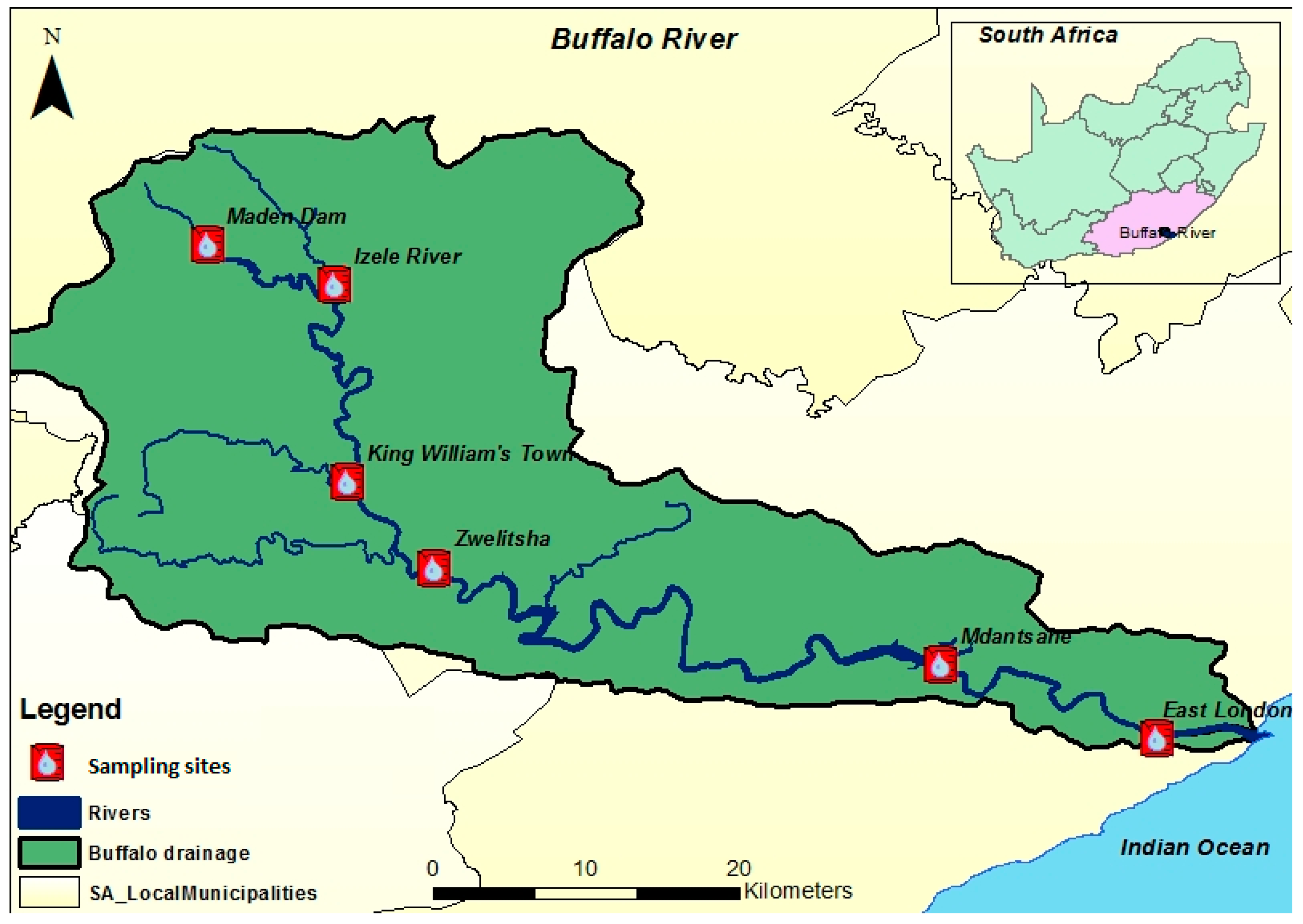
2.1. Description of Study Sites
2.2. Field Sampling
2.3. Chemicals
2.4. Preparation of Sample
2.5. Clean-Up
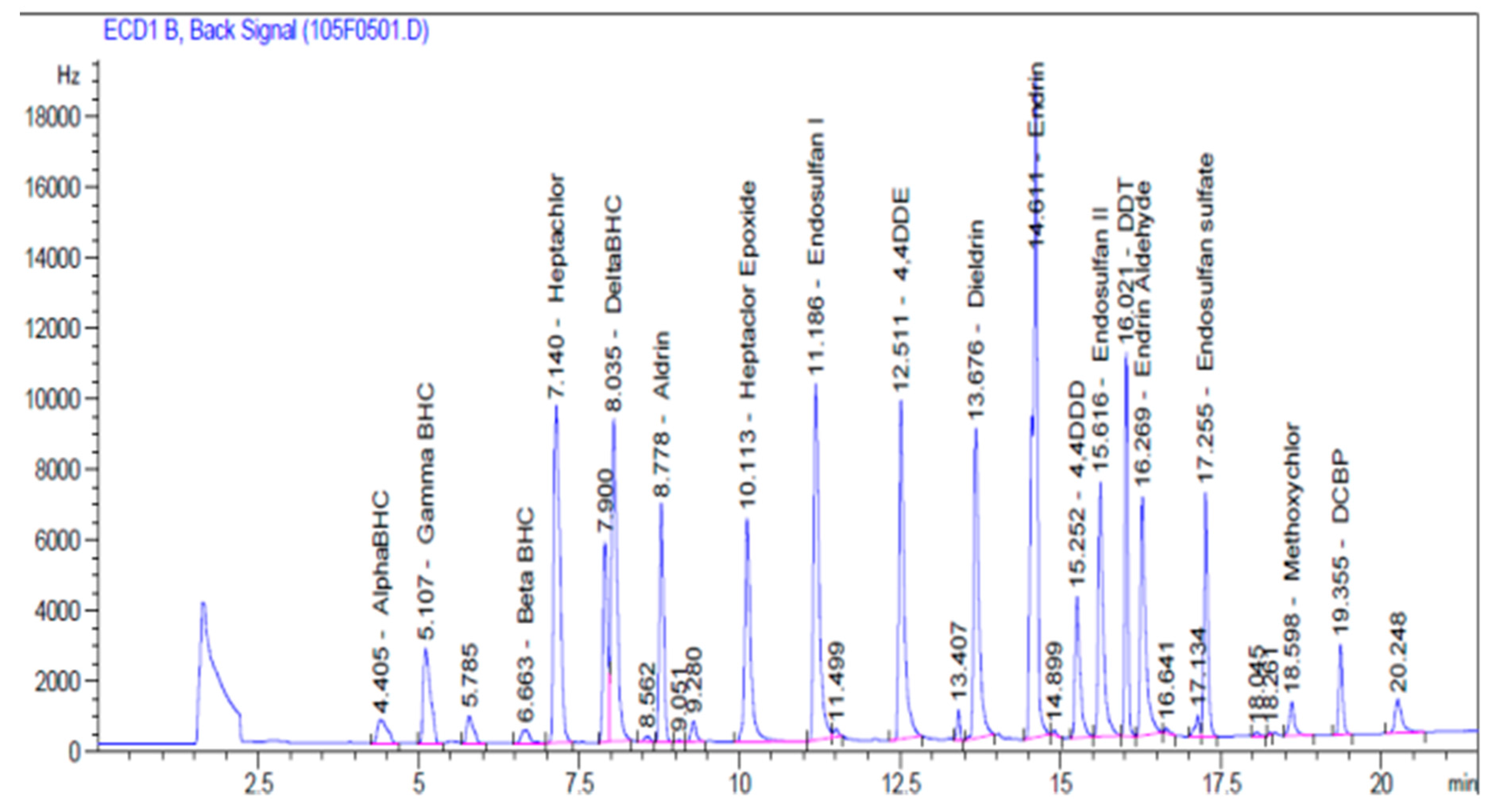
2.6. Instrumental Analysis
2.7. Quality Assurance
2.8. Statistical Analysis
2.9. Risk Assessments
3. Results and Discussion
3.1. Results
3.1.1. Quality Assurance
3.1.2. Level of OCPs in the Buffalo River
3.2. Discussion
3.2.1. Quality Assurance
3.2.2. Level of OCPs
3.2.3. Risk Assessment
4. Conclusions
Acknowledgments
Author Contributions
Conflicts of Interest
References
- Guo, Y.; Meng, X.Z.; Tang, H.L.; Zeng, E.Y. Tissue distribution of organochlorine pesticides in fish collected from the Pearl River delta, China: Implications for fishery input source and bioaccumulation. Environ. Pollut. 2008, 155, 150–156. [Google Scholar] [CrossRef] [PubMed]
- Zhi, H.; Zhao, Z.; Zhang, L. The fate of polycyclic aromatic hydrocarbons (PAHs) and organochlorine pesticides (OCPs) in water from Poyang Lake, the largest freshwater lake in China. Chemosphere 2015, 119, 1134–1140. [Google Scholar] [CrossRef] [PubMed]
- Sun, Y.X.; Hao, Q.; Xu, X.R.; Luo, X.J.; Wang, S.L.; Zhang, Z.W.; Mai, B.X. Persistent organic pollutants in marine fish from Yongxing Island, South China Sea: Levels, composition profiles and human dietary exposure assessment. Chemosphere 2014, 98, 84–90. [Google Scholar] [CrossRef] [PubMed]
- Bouraie, M.M.; EL-Barbary, A.A.; Yehia, M. Determination of Organochlorine Pesticide (OCPs) in Observation Wells from El-Rahawy Contaminated Area, Egypt. Environ. Res. Eng. Manag. 2011, 3, 28–38. [Google Scholar]
- Sibali, L.L.; Okwonkwo, J.O.; McCrindle, R.I. Determination of selected organochlorine pesticide (OCP) compounds from the Jukskei River catchment area in Gauteng, South Africa. Water SA 2008, 34, 611–621. [Google Scholar]
- Amdany, R.; Chimuka, L.; Cukrowska, E.; Kukučka, P.; Kohoutek, J.; Vrana, B. Investigating the temporal trends in PAH, PCB and OCP concentrations in Hartbeespoort Dam, South Africa, using semipermeable membrane devices (SPMDs). Environ. Monit. Assess. 2014, 40, 425–436. [Google Scholar] [CrossRef]
- Eqani, S.A.; Naseem, R.; Cincinelli, A.; Zhang, G.; Mohammad, A.; Qadir, A.; Rashid, A.; Bokhari, H.; Jones, K.C.; Katsoyiannis, A. Uptake of organochlorine pesticides (OCPs) and polychlorinated biphenyls (PCBs) by river water fish: The case of River Chenab. Sci. Total Environ. 2013, 450–451, 83–91. [Google Scholar] [CrossRef] [PubMed]
- Karacik, B.; Okay, O.S.; Henkelmann, B.; Pfister, G.; Schramm, K.W. Water concentrations of PAH, PCB and OCP by using semipermeable membrane devices and sediments. Mar. Pollut. Bull. 2013, 70, 258–265. [Google Scholar] [CrossRef] [PubMed]
- Eskenazi, B.; Marks, A.R.; Bradman, A.; Fenster, L.; Johnson, C.; Barr, D.B.; Jewel, N.P. In utero exposure to dichlorodiphenyltrichloroethane (DDT) and dichlorodiphenyldichloroethylene (DDE) and neurodevelopment among young Mexican American children. Paediatrics 2006, 118, 233–241. [Google Scholar] [CrossRef] [PubMed]
- ASTDR (Agency for Toxic Substances and Disease Registry). Chemical and Physical Information. 2009. Available online: https://www.atsdr.cdc.gov/toxprofiles/tp200.pdf (accessed on 20 September 2017).
- Tiemann, U. In vivo and in vitro effects of the organochlorine pesticides DDT, TCPM, methoxychlor, and lindane on the female reproductive tract of mammals: A review. Reprod. Toxicol. 2008, 25, 316–326. [Google Scholar] [CrossRef] [PubMed]
- Afful, S.; Anim, A.K.; Serfor-Armah, Y. Spectrum of organochlorine pesticide residues in fish samples from the Densu Basin. Res. J. Environ. Earth Sci. 2010, 2, 133–138. [Google Scholar]
- Adeyemi, D.; Ukpo, G.; Anyakora, C.; Unyimadu, J.P. Organochlorine pesticide residues in fish samples from Lagos Lagoon, Nigeria. Am. J. Environ. Sci. 2008, 4, 649–653. [Google Scholar] [CrossRef]
- Kafilzadeh, F.; Ebrahimnezhad, M.; Tahery, Y. Isolation and Identification of Endosulfan-Degrading Bacteria and Evaluation of Their Bioremediation in Kor River, Iran. Osong Public Health Res. Perspect. 2015, 6, 39–46. [Google Scholar] [CrossRef] [PubMed]
- Pawelczyk, A. Assessment of health risk associated with persistent organic pollutants in water. Environ Monit. Assess. 2013, 185, 497–508. [Google Scholar] [CrossRef] [PubMed]
- Farina, Y.; Abdullah, M.P.; Bibi, N.; Khalik, W.W. Pesticides Residues in Agricultural Soils and Its Health Assessment for Humans in Cameron Highlands, Malaysia. Malays. J. Anal. Sci. 2016, 20, 1346–1358. [Google Scholar] [CrossRef]
- Sabaliunas, D.; Sodergren, A. Use of semipermeable membrane devices to monitor pollutants in water and assess their effects: A laboratory test and field verification. Environ. Pollut. 1997, 96, 195–205. [Google Scholar] [CrossRef]
- Meyer, J.L.; Kaplan, L.A.; Newbold, D.; Strayer, D.L.; Woltemade, C.J.; Zedler, J.B.; Beilfuss, R.; Carpenter, Q.; Semlitsch, R.; Watzin, M.C.; et al. Where rivers are born: The Scientific Imperative for Defending Small Streams and Wetlands. Reducing impacts of agriculture at the watershed scale. Front. Ecol. 2003, 1, 65–72. [Google Scholar]
- Bornman, R.; Jager, C.; Worku, Z.; Farias, P.; Reif, S. DDT and urogenital malformations in newborn boys in a malarial area. BJU Int. 2010, 106, 405–411. [Google Scholar] [CrossRef] [PubMed]
- Dallas, H. Water temperature and riverine ecosystems: An overview of knowledge and approaches for assessing biotic responses, with special reference to South Africa. Water SA 2008, 3, 34. [Google Scholar]
- Fatoki, O.S.; Awofolu, O.R. Persistent organochlorine pesticide residues in freshwater systems and sediments from the Eastern Cape, South Africa. Water SA 2004, 29. [Google Scholar] [CrossRef]
- Maharaj, S. Modeling the Behaviour and Fate of Priority Pesticides in South Africa. Master’s Thesis, University of the Western Cape, Cape Town, South Africa, 2005. [Google Scholar]
- Kwok, K.W.H.; Leung, K.M.Y.; Lui, G.S.G.; Chu, V.K.H.; Lam, P.K.S.; Morritt, D.; Maltby, L.; Brock, T.C.M.; van den Brink, P.J.; Warne, M.S.J.; et al. Comparison of tropical and temperate freshwater animal species’ acute sensitivities to chemicals: Implications for deriving safe extrapolation factors. Integr. Environ. Assess. Manag. 2007, 3, 49–67. [Google Scholar] [CrossRef] [PubMed]
- Ansara-Ross, T.M.; Wepener, V.; Brink, P.J.; Ross, M.J. Pesticides in South African fresh waters. Afr. J. Aquat. Sci. 2012, 37, 1–16. [Google Scholar] [CrossRef]
- EOHCES (EOH Coastal and Environmental Services). Report Title: Environmental & Social Management Programme: Bisie Tin Mining Project Report Version: Final Project Number: 216. 2016. Available online: http://alphaminresources.com/wp-content/uploads/2016/09/Bisie_Tin_Environmental_and_Social_Management_Programme.pdf (accessed on 10 October 2017).
- RHP (River Health Programme). Draft Technical Report: Buffalo River Monitoring, Eastern Cape, South Africa. 2004; pp. 1–115. Available online: www.dwaf.gov.za/iwqs/rhp/state_of_rivers/ecape_04/BuffRiverRepFnl.pdf (accessed on 20 December 2014).
- Chigor, V.N.; Sibanda, T.; Okoh, A.I. Variations in the physicochemical characteristics of the Buffalo River in the Eastern Cape Province of South Africa. Environ. Monit. Assess. 2013, 185, 8733–8747. [Google Scholar] [CrossRef] [PubMed]
- Zamxaka, M.; Pironcheva, G.; Nyo, M. Microbiological and physico-chemical assessment of the quality of domestic water sources in selected rural communities of the Eastern Cape Province, South Africa. Water SA 2004, 30, 333–340. [Google Scholar] [CrossRef]
- Adeniji, A.O.; Okoh, O.O.; Okoh, A.I. Analytical Methods for the Determination of the Distribution of Total Petroleum Hydrocarbons in the Water and Sediment of Aquatic Systems: A Review. J. Chem. 2017. [Google Scholar] [CrossRef]
- Moreno-González, R.; Campillo, J.A.; García, V.; León, V.M. Seasonal input of regulated and emerging organic pollutants through surface watercourses to a Mediterranean coastal lagoon. Chemosphere 2013, 92, 247–257. [Google Scholar] [CrossRef] [PubMed]
- USEPA (United State Environmental Protection Agency). Organochlorine Pesticides by Gas Chromatography (Method 8081B), the Scope and Application. 2007. Available online: https://www.epa.gov/sites/production/files/2015-12/documents/8081b.pdf (accessed on 10 October 2016).
- Jang, J.; Li, A. Separation of PCBs and PAHs in sediment samples using silica gel fraction chromatography. Chemosphere 2001, 44, 1439–1445. [Google Scholar] [CrossRef]
- Mohamed, J.; Murimi, S.; Kihampa, C. Degradation of Water Resources by Agricultural Pesticides and Nutrients, Weruweru, Tanzania. Iran. J. Energy Environ. 2014, 5, 192–201. [Google Scholar]
- El-Gawad, A. Chemical constituents, antioxidant and potential allelopathic effect of the essential oil from the aerial parts of Cullen plicata. Artic. Ind. Crops Prod. 2016, 80, 36–41. [Google Scholar] [CrossRef]
- Burke, E.R.; Holden, A.J.; Shaw, I.C. A method to determine residue levels of persistent organochlorine pesticides in human milk from Indonesia women. Chemosphere 2003, 50, 529–535. [Google Scholar] [CrossRef]
- Ge, J.; Woodward, L.A.; Li, Q.X.; Wang, J. Occurrence, distribution and seasonal variations of polychlorinated biphenyls and polybrominated diphenyl ethers in surface waters of the East Lake, China. Chemosphere 2014, 103, 256–262. [Google Scholar] [CrossRef] [PubMed]
- Pérez-Carrera, E.; León, V.M.L.; Parra, A.G.; González-Mazo, E. Simultaneous determination of pesticides, polycyclic aromatic hydrocarbons and polychlorinated biphenyls in seawater and interstitial marine water samples, using stir bar sorptive extraction-thermal desorption-gas chromatography-mass spectrometry. J. Chromatogr. A 2007, 1170, 82–90. [Google Scholar] [CrossRef] [PubMed]
- Macdonald, S.J. Solvent Exchange from Dichloromethane to n-Hexanes Using the DryVap Concentrator. Available online: http://www.horizontechinc.com/wp/wp-content/uploads/2015/10/AN048_090820_Solvent_Exchange_DryVap.pdf (accessed on 10 November 2017).
- Michael Ebitson. Extracting Organochlorine Pesticides from Water with Atlantic™ HLB-M Disks Horizon Technology, Inc., Salem, NH 2007. Available online: https://www.google.com.hk/url?sa=t&rct=j&q=&esrc=s&source=web&cd=1&ved=0ahUKEwiQkuOV9rLXAhXF0RQKHQbNBL0QFggmMAA&url=http%3A%2F%2Fwww.horizontechinc.com%2FPDF%2F03079_9972997%2FApplicationsNotes%2FAN067_101230_EPA_Method_8081_Pesticides_HLB-M.pdf&usg=AOvVaw3D3w9KmRH25BWgvk1f1I0N (accessed on 10 October 2016).
- Fatoki, O.S.; Awofolu, R.O. Methods for selective determination of persistent organochlorine pesticide residues in water and sediments by capillary gas chromatography and electron-capture detection. J. Chromatogr. A 2003, 983, 225–236. [Google Scholar] [CrossRef]
- Cortes, J.E.; Suspes, A.; Roa, S.; González, C.; Castro, H.E. Total petroleum hydrocarbons by gas chromatography in Colombian Waters and Soils. Am. J. Environ. Sci. 2012, 8, 396–402. [Google Scholar]
- Smith, D.L.K. Evaluating CLP and EPA Methods for Pesticides in Water Using Agilent J&W DB-CLP1/DB-CLP2 GC Columns. Appl. Note 2012, 1–14. Available online: https://www.agilent.com/cs/library/applications/5990-6236EN.pdf (accessed on 14 July 2015).
- Sibiya, P.N. Modification, Development and Application of Extraction Methods for PAHs in Sediments and Water; University of the Witwatersrand: Johannesburg, South Africa, 2012. [Google Scholar]
- Hope, B.; Scatolini, S.; Titust, E.; Cotter, J. Distribution Patterns of Polychlorinnted Biphenyl Congeners in Water, Sediment and Biota from Midway Atoll (North Pacific Ocean). Mar. Pollut. Bull. 1997, 34, 548–563. [Google Scholar] [CrossRef]
- Kumar, B.; Verma, V.K.; Sharma, C.S.; Akolkar, A.B. Quick and easy method for determination of priority phenolic compounds in water and wastewater. J. Xenobiot. 2014, 4, 46–52. [Google Scholar] [CrossRef]
- WDNR (Wisconsin Department of Natural Resources). Analytical Detection Limit Guidance and Laboratory Guide for Determining Method Detection Limits. 1996; PUBL-TS-056-96. Available online: http://dnr.wi.gov/regulations/labcert/documents/guidance/-lodguide.pdf (accessed on 5 October 2017).
- Caruso, A.; Santoro, M. Detection of Organochlorine Pesticides by GC-ECD Following U.S. EPA Method 8081; Thermo Fisher Scientific Inc.: Milan, Italy, 2014; pp. 1–4. [Google Scholar]
- Megahed, A.M.; Dahshan, H.; Abd-El-Kader, M.A.; Abd-Elall, A.M.M.; Elbana, M.H.; Nabawy, E.; Mahmoud, H.A. Polychlorinated biphenyls water pollution along the River Nile, Egypt. Sci. World J. 2015, 1–8. [Google Scholar] [CrossRef] [PubMed]
- EPA (Environmental Protection Agency). Risk Assessment Guidance for Superfund, Human Health Evaluation Manual (Part A). 1989; Volume 1. Available online: http://www.epa.gov/oswer/risk assessment/ragsa/pdf/rags-vol1-pta_complete.pdf (accessed on 29 August 2016).
- Lohmann, R.; Breivik, K.; Dachs, J.; Muir, D. Global fate of POPs: Current and future research directions. Environ. Pollut. 2007, 150, 150–165. [Google Scholar] [CrossRef] [PubMed]
- ECETOC. Guidance for Effective Use of Human Exposure Data in Risk Assessment of Chemicals. 2016. Available online: www.ecetoc.org/2016/ECETOC-TR-126-Guidance-for-Effective-Use-of-Human (accessed on 5 December 2016).
- Bozek, F.; Adamec, V.; Navratil, J.; Kellner, J.; Bumbova, A.; Dvorak, J.L.B. Health Risk Assessment of Air Contamination Caused by Polycyclic Aromatic Hydrocarbons From Traffic. Energy Environ. Eng. Ser. 2009, 104–108. Available online: http://www.vojenskaskola.cz (accessed on 5 January 2017).
- Hamilton, D.J.; Ambrus, Á.; Dieterle, R.M.; Felsot, A.S.; Harris, C.A.; Holland, P.T.; Katayama, A.; Kurihara, N.; Linders, J.; Unsworth, J.; et al. Regulatory limits for pesticide residues in water (IUPAC Technical Report). Pure Appl. Chem. 2003, 75, 1123–1155. [Google Scholar] [CrossRef]
- ECETOC Exposure Factors Sourcebook for European Population. 2001. Available online: www.ecetoc.org/wp-content/uploads/2014/08/ECETOC-TR-079.pdf (accessed on 5 December 2016).
- USEPA-IRIS (United States Environmental Protection Agency—Integrated Risk Information System). National Center for Environmental Assessment, Chemical Assessment Summary. 2014; pp. 1–36. Available online: http://www.epa.gov/iris/backgrd.html (accessed on 6 August 2017).
- USEPA (United States Environmental Protection Agency). National Primary Drinking Water Regulations. 2015; pp. 550–560. Available online: https://www.epa.gov/sites/production/files/2015-11/documents (accessed on 6 August 2017).
- AMEC Human Health Risk Assessment Enbridge Northern Gateway Project. 2010. Available online: https://www.ceaa.gc.ca/050/documents_staticpost/human_health_risk_assess ment.pdf (accessed on 5 December 2016).
- Dolatto, R.G.; Messerschmidt, I.; Fraga Pereira, B.; Martinazzo, R.; Abate, G. Preconcentration of polar phenolic compounds from water samples and soil extract by liquid-phase microextraction and determination via liquid chromatography with ultraviolet detection. Talanta 2016, 148, 292–300. [Google Scholar] [CrossRef] [PubMed]
- Vecchiato, M.; Argiriadis, E.; Zambon, S.; Barbante, C.; Toscano, G.; Gambaro, A.; Piazza, R. Persistent Organic Pollutants (POPs) in Antarctica: Occurrence in continental and coastal surface snow. Microchem. J. 2015, 119, 75–82. [Google Scholar] [CrossRef]
- Tahboub, R.Y.; Zaater, F.M.; Barri, A.T. Simultaneous identification and quantitation of selected organochlorine pesticide residues in honey by full-scan gas chromatography–mass spectrometry. Anal. Chim. Acta 2006, 558, 62–68. [Google Scholar] [CrossRef]
- Sailaukhanuly, Y.; Carlsen, L. Distribution and risk assessment of selected organochlorine pesticides in Kyzyl Kairat village from Kazakhstan. Environ. Monit. Assess. 2016. [Google Scholar] [CrossRef] [PubMed]
- Poolpak, T.; Pokethitiyook, P.; Kruatrachue, M.; Arjarasirikoon, U.; Thanwaniwat, N. Residue analysis of organochlorine pesticides in the Mae Klong river of Central Thailand. J. Hazard. Mater. 2008, 156, 230–239. [Google Scholar] [CrossRef] [PubMed]
- Vassilakis, I.; Tsipi, D.; Scoullos, M. Determination of a variety of chemical classes of pesticides in surface and ground waters by off-line solid-phase extraction, gas chromatography with electron-capture and nitrogen—Phosphorus detection, and high-performance liquid chromatography. J. Chromatogr. A 1998, 823, 49–58. [Google Scholar] [CrossRef]
- Aguilar, C.; Borrull, F.; Marc, R.M. Determination of pesticides in environmental waters by solid-phase extraction and gas chromatography with electron-capture and mass spectrometry detection. J. Chromatogr. A 1997, 771, 221–231. [Google Scholar] [CrossRef]
- Buser, A.; Muller, J. Biodegradation of Hexachlorocyclohexane in the Environment. 1995. Chapter 3.9. pp. 153–161. Available online: https://books.google.co.za/books (accessed on 4 October 2017).
- Lohmann, R.; Belkin, I. Organic pollutants and ocean fronts. Prog. Oceanogr. 2012, 128, 172–184. [Google Scholar] [CrossRef]
- Barber, J.L.; Sweetman, A.J.; Wijk, V.D.; Jones, K.C. Hexachlorobenzene in the global environment: Emissions, levels, distribution, trends and processes. Sci. Total Environ. 2005, 349, 1–44. [Google Scholar] [CrossRef] [PubMed]
- Quinn, L.P.; Vos, J.; Roos, C.; Bouwman, H.; Kylin, H.; Pieters, R.; Berg, J.; Van Den, B.J. Pesticide Use in South Africa: One of the Largest Importers of Pesticides in Africa. Pesticides Mod World-Pesticides Use Management 2011. pp. 1–48. Available online: www.intechopen.com (accessed on 10 December 2015).
- Yadav, I.C.; Devi, N.L.; Syed, J.H.; Cheng, Z.; Li, J.; Zhang, G.; Jones, K.C. Current status of persistent organic pesticides residues in air, water, and soil, and their possible effect on neighboring countries: A comprehensive review of India. Sci. Total Environ. 2015, 511, 123–137. [Google Scholar] [CrossRef] [PubMed]
- Sarkar, S.K.; Binelli, A.; Riva, C.; Parolini, M.; Chatterjee, M.; Bhattacharya, A.K.; Bhattacharya, B.D.; Satpathy, K.K. Organochlorine pesticide residues in sediment cores of Sunderban wetland, northeastern part of bay of Bengal, India, and their ecotoxicological significance. Arch. Environ. Contam. Toxicol. 2008. [Google Scholar] [CrossRef] [PubMed]
- Zulin, Z.; Huasheng, H.; Xinhong, W.; Jianqing, L.; Weiqi, C.; Li, X. Determination and load of organophosphorus and organochlorine pesticides at water from Jiulong River Estuary, China. Mar. Pollut. Bull. 2002, 45, 397–402. [Google Scholar] [CrossRef]
- Melymuk, L.; Kukucka, P.; Kuku, P. Distribution of legacy and emerging semivolatile organic compounds in five indoor matrices in a residential environment. Chemosphere 2016. [Google Scholar] [CrossRef] [PubMed]
- Liu, X.; Ming, L.L.; Nizzetto, L.; Borgå, K.; Larssen, T.; Zheng, Q.; Li, J.; Zhang, G. Critical evaluation of a new passive exchange-meter for assessing multimedia fate of persistent organic pollutants at the air-soil interface. Environ. Pollut. 2013, 181, 144–150. [Google Scholar] [CrossRef] [PubMed]
- Muir, D.C.G.; De Wit, C.A. Trends of legacy and new persistent organic pollutants in the circumpolar arctic: Overview, conclusions, and recommendations. Sci. Total Environ. 2010, 408, 3044–3051. [Google Scholar] [CrossRef] [PubMed]
- Miguel, N.; Ormad, M.P.; Mosteo, R.; Ovelleiro, J.L. Photocatalytic Degradation of Pesticides in Natural Water: Effect of Hydrogen Peroxide. Int. J. Photoenergy 2012, 2012. [Google Scholar] [CrossRef]
- Bulut, S.; Erdoðmuþ, S.F.; Konuk, M.; Cemek, M. The Organochlorine Pesticide Residues in the Drinking Waters of Afyonkarahisar, Turkey. Ekoloji 2010, 19, 24–31. [Google Scholar]
- Williams, A.B. Residue analysis of organochlorine pesticides in water and sediments from Agboyi Creek, Lagos. Acad. J. 2013, 7, 267–273. [Google Scholar]
- USEPA (United States Environmental Protection Agency). Drinking Water Standards and Health Advisories 2012. pp. 1–20. Available online: http://water.epa.gov/action/advisories/drinking/upload/dwstandards2012 (accessed on 10 October 2016).
- Spadoni, G.; Morra, P.; Bagli, S. The analysis of human health risk with a detailed procedure operating in a GIS environment. Environ. Int. 2006, 32, 444–454. [Google Scholar]
- USEPA (United States Environmental Protection Agency). National Primary and Secondary Drinking Water Regulations. 2009. Available online: http://www.epa.gov/safewater/EPA 816-F-09-004 (accessed on 10 October 2016).
- Källqvist, T.; Thomas, K.; Sorensen, Q. Environmental Risk Assessment of Artificial Turf Systems. Norwegian Institute for Water Research, 2005; pp. 1–20. Available online: www.isss-sportsurfacescience.org/downloads/documents/5veu2czb25_nivaengelsk.pd (accessed on 20 March 2017).
- USEPA (United State Environmental Protection Agency). Guidelines for Carcinogen Risk Assessment. 2005. Available online: https://www.epa.gov/sites/production/files/2013-09/documents/cancer_guidelines_final_3-25-05.pdf (accessed on 20 October 2016).


| Sampling Site | Latitude | Longitude | Description of Sites |
|---|---|---|---|
| Buffalo River Estuary (BRE) | 33°1′26.06″ S | 27°53′26.41″ E | Municipal and industrial effluent discharged, including agricultural run-offs. |
| Mdantsane (MSN) | 32°58′50.94″ S | 27°42′28.78″ E | Sewerage works, heaps of refuse at the dump and the Potsdam treatment works and food factories. |
| Zwelitsha (ZW) | 32°55′48.97″ S | 27°25′59.31″ E | Influx of wastes from agricultural farm lands, refuse dumpsites, sewerage outfalls and aerated treatment pond. |
| King William’s Town (KWT) | 32°52′44.06″ S | 27°22′54.89″ E | Hazardous industrial and domestic wastes as well as agricultural run-offs are discharged. |
| Izele River (IZ) | 32°45′52.32″ S | 27°22′22.42″ E | Domestic wastes and agricultural run-offs are discharged. |
| Maden Dam (MD) | 32°44′26.15″ S | 27°17′59.47″ E | Pristine but at times cattle grazing |
| OCPs | Retention Time (min) | Equation | r2 |
|---|---|---|---|
| α-BHC | 4.405 | y = 13833x | 0.9951 |
| γ-BHC | 5.107 | y = 64859x | 0.9956 |
| β-BHC | 6.663 | y = 99379x | 0.9928 |
| Heptachlor | 7.140 | y = 207701x | 0.9886 |
| δ-BHC | 8.035 | y = 186188x | 0.9924 |
| Aldrin | 8.778 | y = 107562x | 0.9938 |
| Heptachlor epoxide | 10.113 | y = 130345x | 0.9887 |
| Endosulfan I | 11.186 | y = 192696x | 0.9962 |
| 4,4-DDE | 12.511 | y = 172980x | 0.9937 |
| Dieldrin | 13.676 | y = 155561x | 0.9937 |
| Endrin | 14.611 | y = 326806x | 0.9969 |
| 4,4-DDD | 15.252 | y = 64298x | 0.9949 |
| Endosulfan II | 15.616 | y = 124856x | 0.9884 |
| 4,4-DDT | 16.021 | y = 118677x | 0.9975 |
| Enrin Aldehyde | 16.269 | y = 129680x | 0.9916 |
| Endosulfan Sulfate | 17.255 | y = 95893x | 0.9913 |
| Methoxychlor | 18.598 | y = 18172x | 0.9959 |
| DCBP | 19.355 | y = 35257x | 0.9886 |
| OCPs | Sampling Points | Range | |||||||||||
|---|---|---|---|---|---|---|---|---|---|---|---|---|---|
| BRE | FD | MSN | FD | ZW | FD | KWT | FD | IZ | FD | MD | FD | ||
| α-BHC | 446 ± 0.11 | 100 | 684 ± 0.27 | 100 | 1476 0.08 | 33 | <LOD | 0 | <LOD | 0 | <LOD | 0 | <LOD–1476 |
| γ-BHC | <LOD | 0 | <LOD | 0 | 127 ± 0.01 | 33 | <LOD | 0 | <LOD | 0 | <LOD | 0 | <LOD–127 |
| β-BHC | 170 ± 0.04 | 100 | 654 ± 0.56 | 67 | 218 ± 0.07 | 100 | 4403 ± 0.02 | 33 | <LOD | 0 | <LOD | 0 | <LOD–4403 |
| Heptachlor | <LOD | 0 | 79 ± 0.01 | 100 | 31 ± 0.03 | 33 | 40 ± 0.01 | 33 | <LOD | 0 | <LOD | 0 | <LOD–79 |
| δ-BHC | 34 ± 0.01 | 33 | 56 ± 0.01 | 100 | 78 ± 0.03 | 67 | 46 ± 0.01 | 100 | <LOD | 0 | <LOD | 0 | <LOD–78 |
| Aldrin | 243 ± 0.03 | 100 | 100 ± 0.04 | 100 | 253 ± 0.10 | 100 | 117 ± 0.06 | 100 | 197 ± 0.08 | 67 | 120 ± 0.04 | 100 | 100–253 |
| Hep. Epoxide | 292 ± 0.11 | 100 | 54 ± 0.02 | 100 | 56 ± 0.01 | 100 | 50 ± 0.01 | 100 | 194 ± 0.12 | 100 | 151 ± 0.16 | 100 | 50–292 |
| Endosulfan I | 48 ± 0.01 | 100 | 43 ± 0.02 | 100 | 63 ± 0.02 | 67 | 57 ± 0.01 | 33 | 389 ± 0.01 | 33 | <LOD | 0 | <LOD–389 |
| 4,4-DDE | <LOD | 0 | <LOD | 0 | 234 ± 0.01 | 67 | <LOD | 0 | <LOD | 0 | <LOD | 0 | <LOD–234 |
| Dieldrin | 86 ± 0.02 | 100 | <LOD | 0 | <LOD | 0 | <LOD | 33 | <LOD | 0 | <LOD | 0 | <LOD–86 |
| Endrin | <LOD | 0 | <LOD | 100 | <LOD | 0 | <LOD | 0 | <LOD | 0 | <LOD | 0 | <LOD |
| 4,4-DDD | 34 ± 0.01 | 100 | 494 ± 0.01 | 67 | 121 ± 0.12 | 67 | <LOD | 0 | 311 | 33 | <LOD | 0 | <LOD–494 |
| Endosulfan II | 30 ± 0.01 | 100 | <LOD | 0 | 60 ± 0.03 | 67 | <LOD | 0 | <LOD | 0 | <LOD | 0 | <LOD–60 |
| 4,4-DDT | <LOD | 33 | <LOD | 67 | 218 ± 0.12 | 67 | <LOD | 33 | <LOD | 33 | <LOD | 0 | <LOD–218 |
| Endrin Alde. | <LOD | 0 | 208 ± 0.01 | 33 | <LOD | 0 | <LOD | 33 | <LOD | 0 | <LOD | 0 | <LOD–208 |
| End. Sulphate | 174 ± 0.03 | 100 | 440 ± 0.06 | 67 | 571 ± 0.07 | 100 | 381 ± 0.12 | 67 | 392 ± 0.04 | 100 | <LOD | 100 | <LOD–571 |
| Methoxychlor | 2080 ± 0.04 | 100 | 113 ± 0.01 | 33 | 576 ± 0.09 | 100 | <LOD | 0 | <LOD | 0 | 164 ± 0.01 | 33 | <LOD–2080 |
| ∑OCPs | 3637 ± 0.42 | - | 2525 ± 0.99 | - | 4148 ± 1.90 | - | 5094 ± 0.26 | - | 1483 ± 0.26 | - | 435 ± 0.21 | - | 435–5094 |
| No. of OCPs | 11 | - | 11 | - | 14 | - | 8 | - | 5 | - | 3 | - | |
| OCPs | Sampling Points | Range | |||||||||||
|---|---|---|---|---|---|---|---|---|---|---|---|---|---|
| BRE | FD | MSN | FD | ZW | FD | KWT | FD | IZ | FD | MD | FD | ||
| α-BHC | 125 ± 0.04 | 100 | 313 ± 0.06 | 100 | 224 ± 0.3 | 100 | 293 ± 0.26 | 100 | 187 ± 0.24 | 100 | 39 ± 0.02 | 33 | 39–313 |
| γ-BHC | <LOD | 0 | <LOD | 0 | 63 ± 0.01 | 33 | <LOD | <LOD | <LOD | 0 | <LOD–63 | ||
| β-BHC | 130 ± 0.07 | 100 | 119 ± 0.01 | 100 | 62 ± 0.4 | 100 | 53± 0.04 | 100 | 127 ± 0.03 | 100 | 87 ± 0.01 | 33 | 53–130 |
| Heptachlor | 127 ± 0.01 | 33 | <LOD | 0 | <LOD | 0 | <LOD | 0 | 93 ± 0.08 | 67 | <LOD | 0 | <LOD–127 |
| δ-BHC | <LOD | 33 | <LOD | 0 | <LOD | 0 | <LOD | 0 | <LOD | 0 | <LOD | 0 | <LOD |
| Aldrin | 30 ± 0.02 | 100 | 85 ± 0.07 | 67 | <LOD | 0 | 97 ± 0.08 | 67 | 143 ± 0.11 | 67 | 57 ± 0.01 | 67 | <LOD–143 |
| Hep. Epoxide | <LOD | 0 | <LOD | 0 | 86 ± 0.05 | 33 | 29 ± 0.01 | 100 | 21 ± 0.01 | 67 | <LOD | 0 | <LOD–86 |
| Endosulfan I | <LOD | 0 | 31 ± 0.01 | 67 | <LOD | 0 | <LOD | 0 | 60 ± 0.02 | 100 | <LOD | 0 | <LOD–60 |
| 4,4-DDE | <LOD | 0 | <LOD | 0 | 201 ± 0.01 | 67 | <LOD | 0 | <LOD | 0 | <LOD | 0 | <LOD–201 |
| Dieldrin | <LOD | 0 | <LOD | 67 | <LOD | 0 | <LOD | 0 | <LOD | 0 | <LOD | 0 | <LOD |
| Endrin | <LOD | 0 | <LOD | 0 | <LOD | 0 | <LOD | 0 | <LOD | 0 | <LOD | 0 | <LOD |
| 4,4-DDD | 36 ± 0.02 | 67 | 79 ± 0.06 | 67 | <LOD | 0 | <LOD | 0 | 53 ± 0.03 | 67 | <LOD | 0 | <LOD–79 |
| Endosulfan II | <LOD | 0 | 222 ± 0.02 | 67 | 154 ± 0.02 | 33 | <LOD | 0 | <LOD | 67 | <LOD | 0 | <LOD–222 |
| 4,4-DDT | <LOD | 0 | 44 ± 0.03 | 67 | <LOD | 0 | <LOD | 0 | 40 ± 0.26 | 67 | <LOD | 0 | <LOD–44 |
| Endrin Alde. | <LOD | 0 | <LOD | 0 | <LOD | 0 | <LOD | 0 | <LOD | 0 | <LOD | 0 | <LOD |
| End. Sulphate | <LOD | 0 | 48 ± 0.04 | 100 | <LOD | 0 | <LOD | 0 | <LOD | 67 | <LOD | 0 | <LOD–48 |
| Methoxychlor | 236 ± 0.4 | 33 | 39 ± 0.3 | 100 | 89 ± 0.07 | 67 | 185 ± 0.16 | 0 | 252 ± 0.2 | 0 | <LOD | 0 | <LOD–252 |
| ∑OCPs | 684 ± 0.54 | - | 978 ± 0.69 | - | 878 ± 0.87 | - | 657 ± 0.55 | - | 976 ± 0.75 | - | 183 ± 0.04 | - | 183–978 |
| No. of OCPs | 6 | - | 9 | - | 7 | - | 6 | - | 9 | - | 3 | - | |
| OCPs | HQ0–6 × 10⁻⁶ | H7–17 × 10−6 | HQAdt × 10−6 |
|---|---|---|---|
| γ-BHC | 7 | 5 | 1 |
| Heptachlor | 55 | 33 | 11 |
| Aldrin | 2013 | 1193 | 403 |
| Heptachlor Epoxide | 3956 | 2344 | 791 |
| 4,4-DDE | 14,751 | 8741 | 2950 |
| Dieldrin | 574 | 340 | 115 |
| 4,4-DDD | 8306 | 4922 | 1661 |
| 4,4-DDT | 12 | 7 | 2 |
| Methoxychlor | 53 | 32 | 11 |
| OCPs | ADD0–6 × 10⁻⁶ | ADD7–17 × 10−6 | ADDadt × 10−6 | LADD0–6&adt × 10−6 | LADD7–17 × 10−6 | Cancer Risk × 10−13 |
|---|---|---|---|---|---|---|
| α-BHC | 269 | 159 | 54 | 231 | 25 | 10 |
| γ-BHC | 39 | 23 | 8 | 33 | 4 | 1.5 |
| β-BHC | 618 | 366 | 124 | 530 | 58 | 24 |
| Heptachlor | 28 | 16 | 6 | 24 | 3 | 1.1 |
| δ-BHC | 22 | 13 | 4 | 18 | 2 | 0.8 |
| Aldrin | 60 | 36 | 13 | 52 | 6 | 2.3 |
| Hept. Epoxide | 51 | 30 | 1 | 44 | 5 | 2.0 |
| Endosulfan I | 54 | 32 | 12 | 46 | 5 | 2.1 |
| 4,4-DDE | 44 | 26 | 9 | 38 | 4 | 1.7 |
| Dieldrin | 29 | 17 | 6 | 25 | 3 | 1.1 |
| Endrin | 0 | 0 | 0 | 0 | 0 | 0 |
| 4,4-DDD | 75 | 44 | 15 | 64 | 7 | 2.9 |
| Endosulfan II | 36 | 22 | 7 | 31 | 3 | 1.4 |
| 4,4-DDT | 58 | 34 | 11 | 50 | 5 | 2.2 |
| Endrin Alde. | 748 | 443 | 150 | 641 | 70 | 28 |
| Endo. Sulfate | 94 | 55 | 19 | 80 | 87 | 3.6 |
| Methoxychlor | 266 | 158 | 53 | 228 | 25 | 10 |
© 2017 by the authors. Licensee MDPI, Basel, Switzerland. This article is an open access article distributed under the terms and conditions of the Creative Commons Attribution (CC BY) license (http://creativecommons.org/licenses/by/4.0/).
Share and Cite
Yahaya, A.; Okoh, O.O.; Okoh, A.I.; Adeniji, A.O. Occurrences of Organochlorine Pesticides along the Course of the Buffalo River in the Eastern Cape of South Africa and Its Health Implications. Int. J. Environ. Res. Public Health 2017, 14, 1372. https://doi.org/10.3390/ijerph14111372
Yahaya A, Okoh OO, Okoh AI, Adeniji AO. Occurrences of Organochlorine Pesticides along the Course of the Buffalo River in the Eastern Cape of South Africa and Its Health Implications. International Journal of Environmental Research and Public Health. 2017; 14(11):1372. https://doi.org/10.3390/ijerph14111372
Chicago/Turabian StyleYahaya, Abdulrazaq, Omobola O. Okoh, Anthony I. Okoh, and Abiodun O. Adeniji. 2017. "Occurrences of Organochlorine Pesticides along the Course of the Buffalo River in the Eastern Cape of South Africa and Its Health Implications" International Journal of Environmental Research and Public Health 14, no. 11: 1372. https://doi.org/10.3390/ijerph14111372