Identification of a Group’s Physiological Synchronization with Earth’s Magnetic Field


Abstract
:1. Introduction
2. Methods and Procedures
2.1. Participants
2.2. Ethics Statement
2.3. Computational Estimation of the Synchronization of a Group’s HRV Time Series with Earth’s Magnetic Field Data
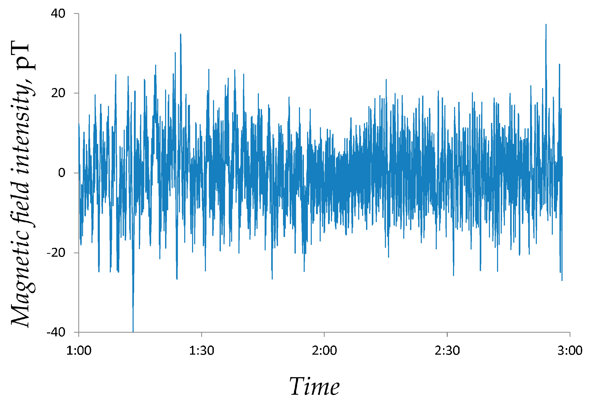
2.3.1. Magnetic Field Data
2.4. Computation of the Power of Local Magnetic Field
- (1)
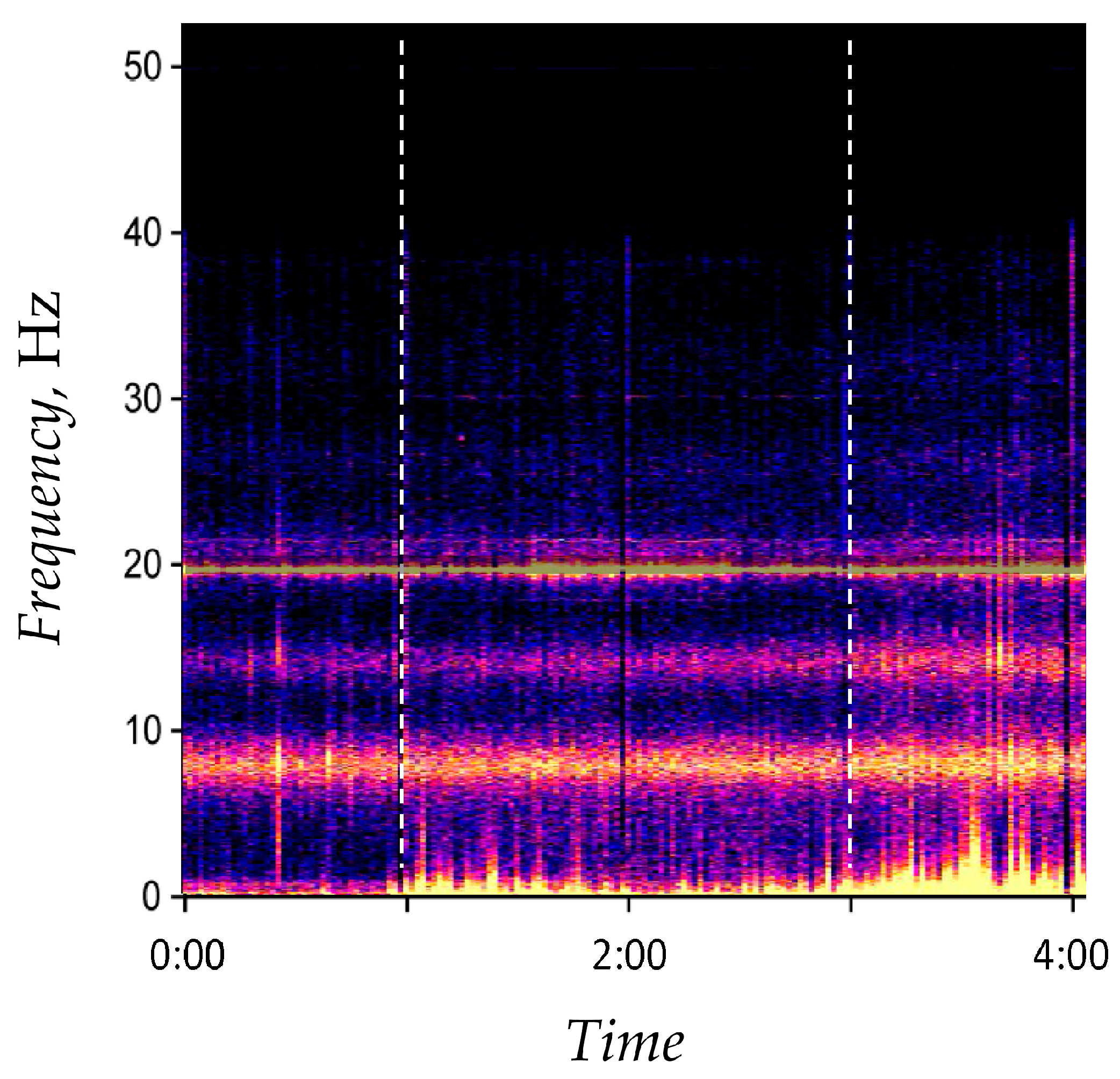
- Compute the spectrogram (as described previously).
- (2)
- Crop the spectrogram in order to eliminate intermittent chaotic outbreaks in the measured data due to manmade noise, lightening, etc.
- (3)
- Apply the Gaussian median filter of dimensions to for the reduction of noise.
- (4)
- Compute the signal power as .
2.4.1. Example: Computation of the Local Magnetic Field Power
2.5. Algorithm for the Computation of Geometrical Synchronization between Two Time Series
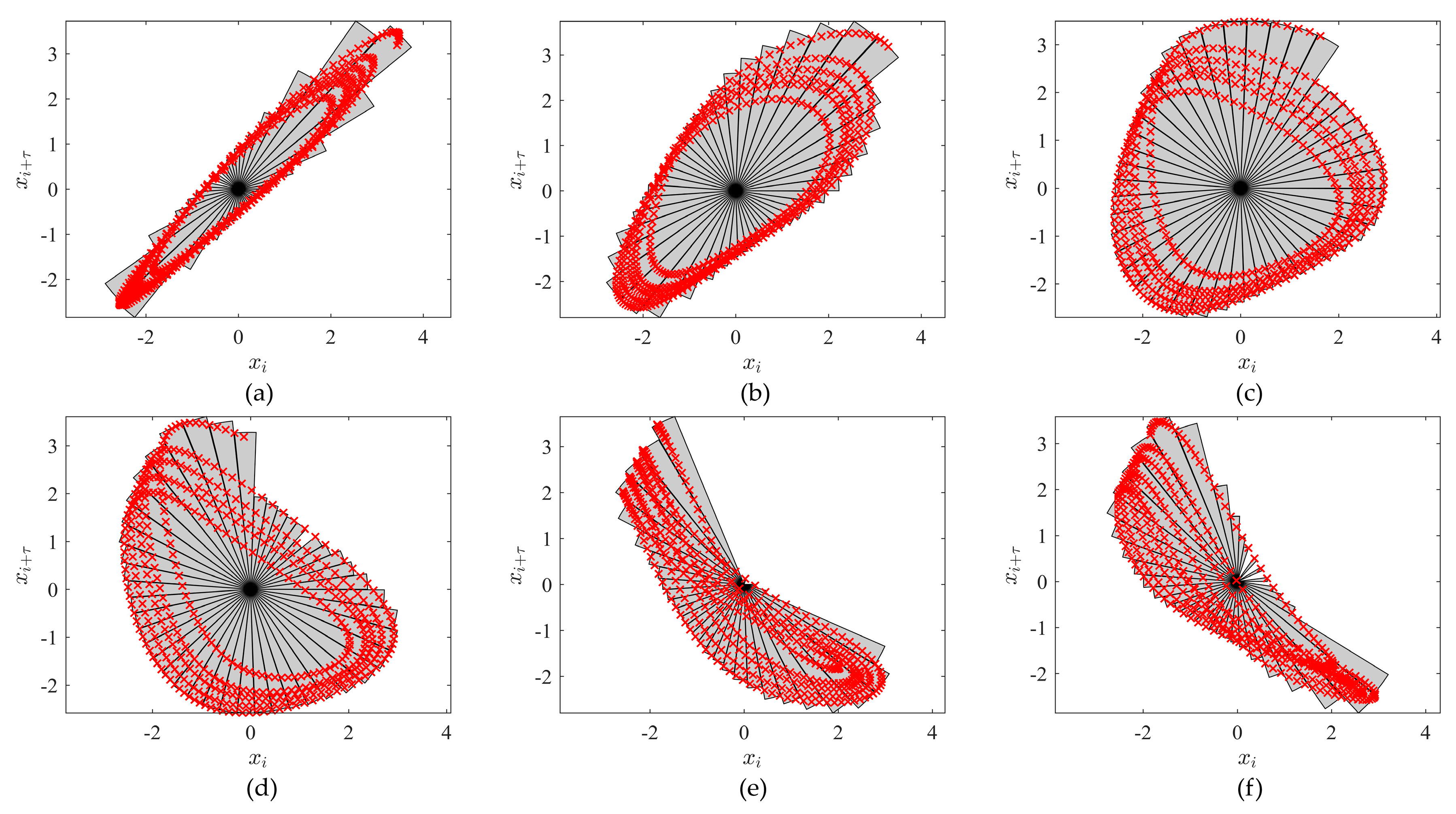
2.5.1. Computation of the Area of an Attractor in the State Space
- (1)
- Compute the center of the mass of the points comprising the attractor. Move the origin of the state space to the center of the mass.
- (2)
- Divide the state space of the attractor into the slices with equal central angles of a circle centered on the origin. The number of slices depends on the number of points in the observation window of the time series.
- (3)
- Set the radius of each slice to the maximal distance between a point belonging to that slice and the origin.
- (4)
- Compute the area of the attractor as the sum of areas of all slices.
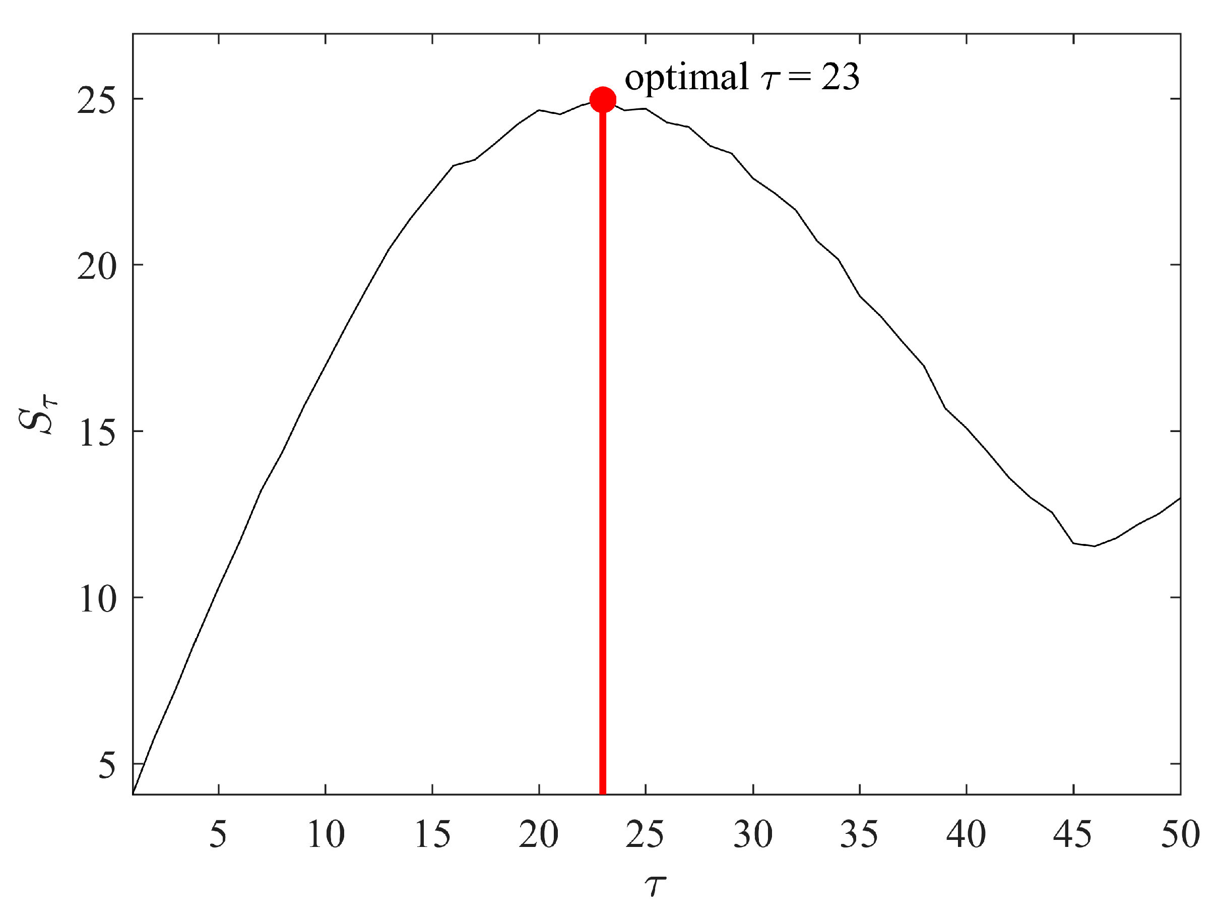
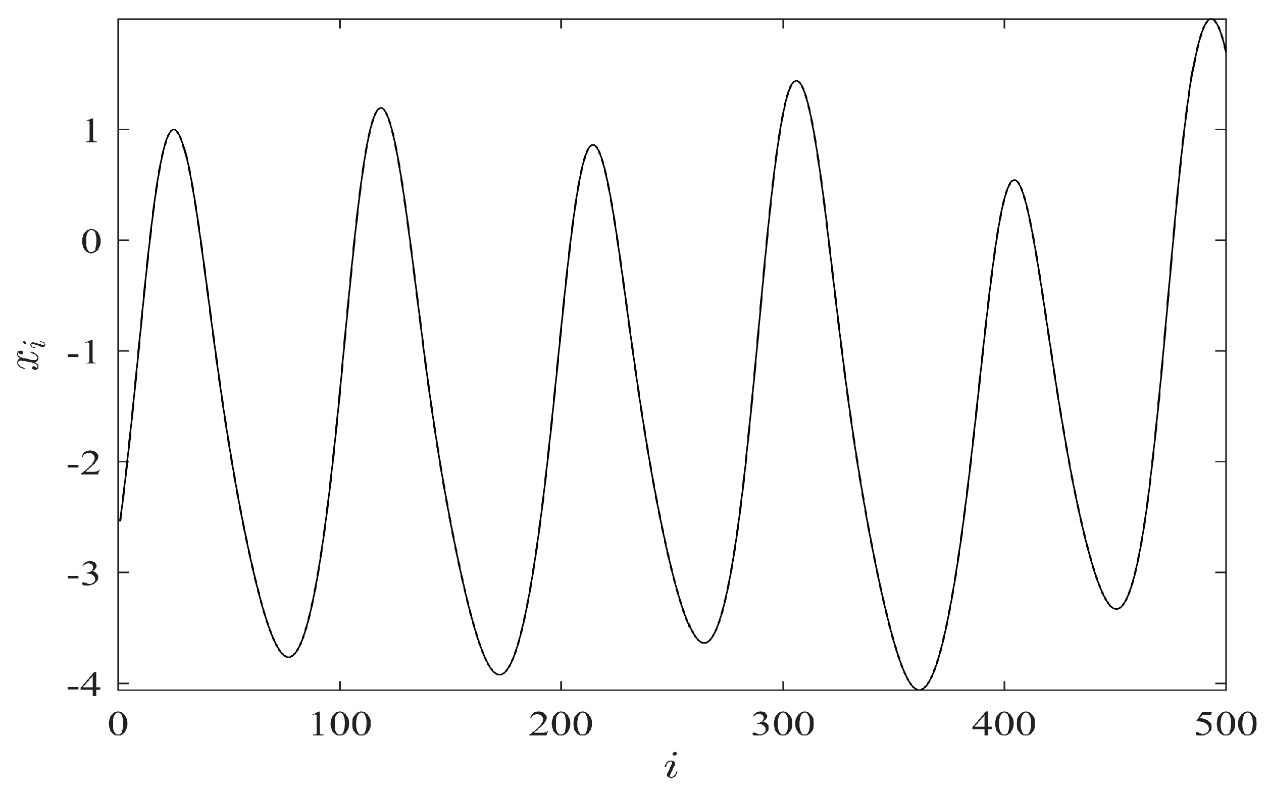
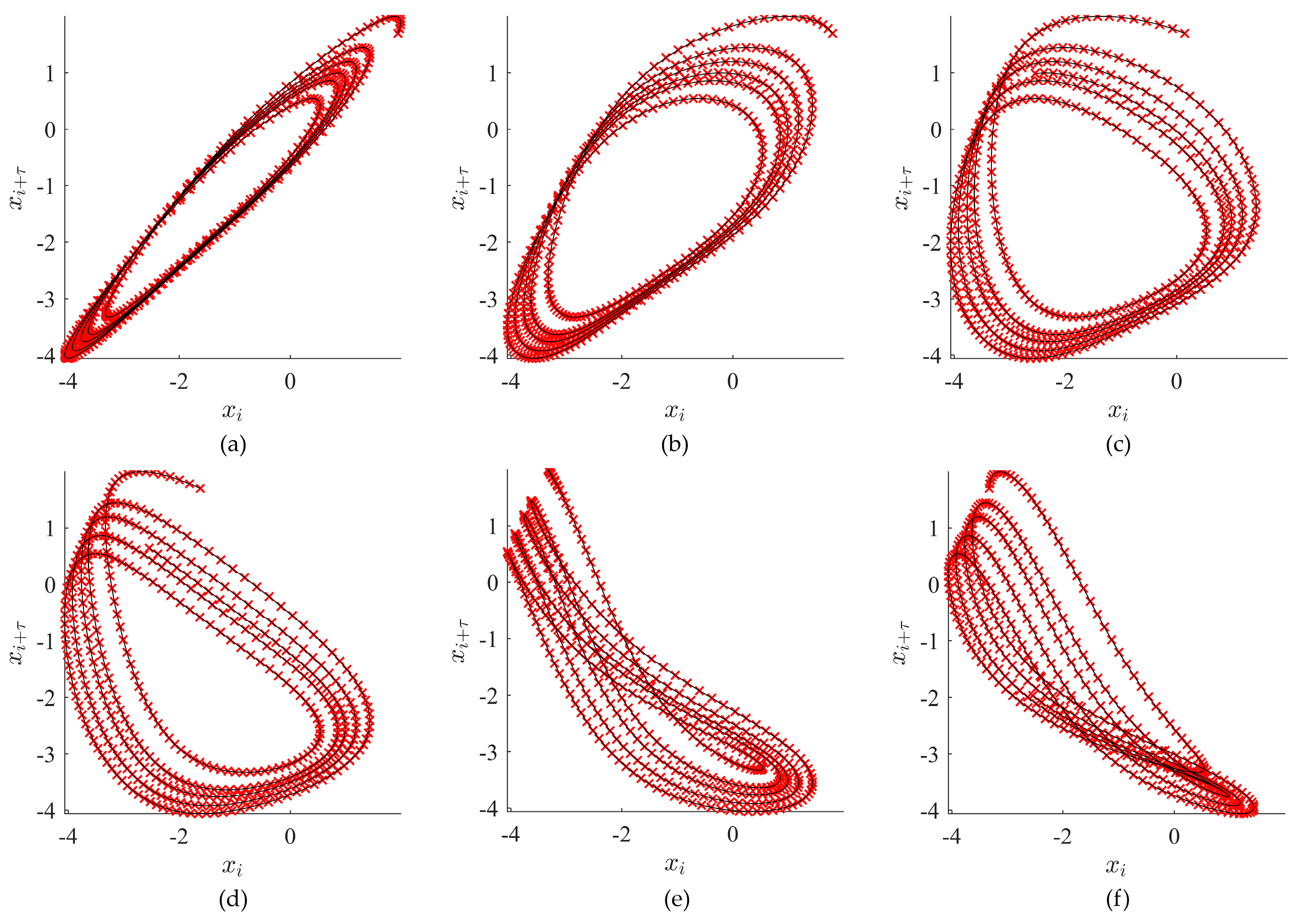
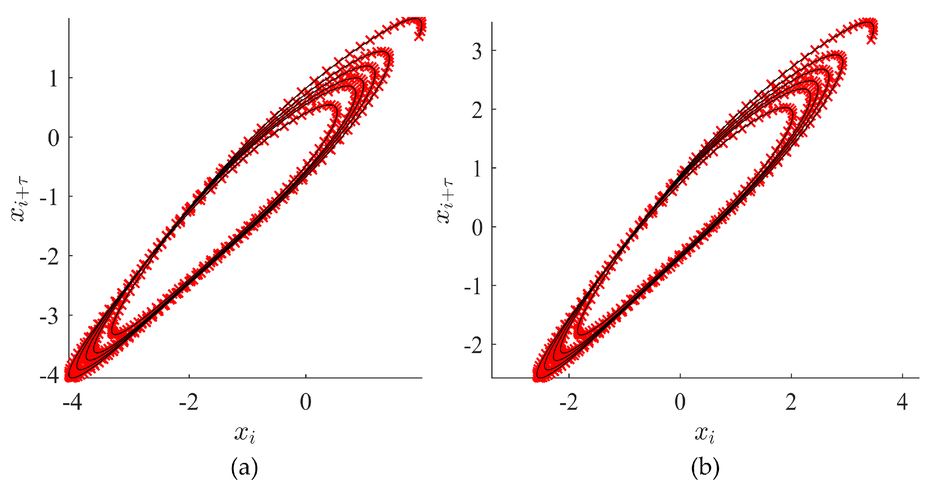
2.5.2. Example 1: Identification of the Optimal Time Lag
2.5.3. Construction of the Algorithm for the Estimation of the Geometrical Synchronization between Two Time Series
- (1)
- Divide signals and into observation windows of size ( should be large enough to enable the reconstruction of a meaningful attractor in the state space):
- (2)
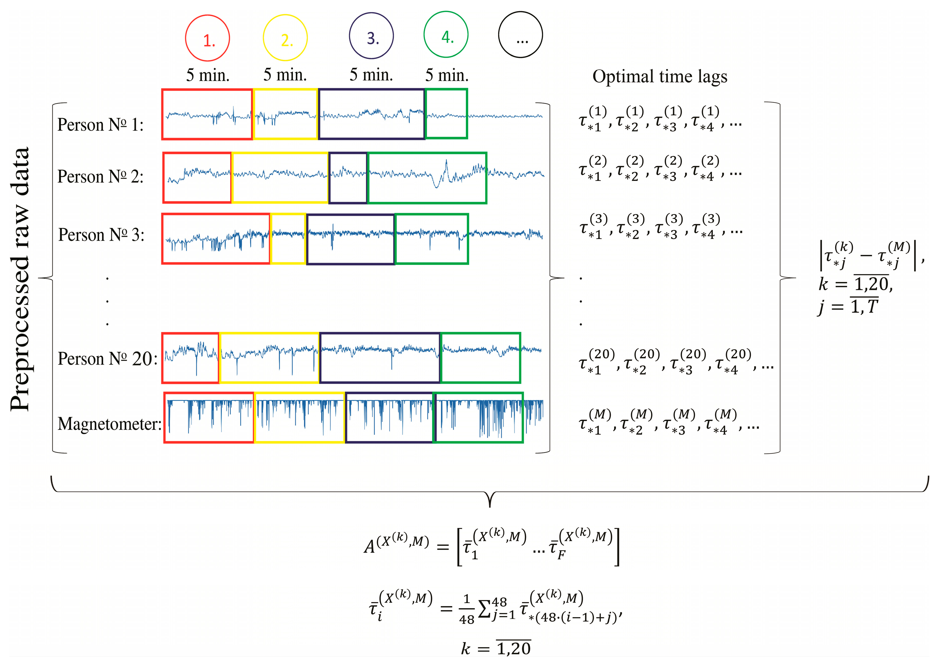
- Compute optimal time lags for each observation window for both time series using Algorithm B. Such computations result in two vectors of optimal time lags: . This information reduction algorithm allows the identification of similarities between attractors reconstructed from different time series from the geometrical point of view. The variation of optimal time lags reconstructed for a pair of time series is used for the quantification of the generalized geometrical synchronization between those time series.
- (3)
- Calculate the vector of absolute differences between obtained optimal time lags for each observation window: . The differences between the optimal time lags are used as the metric of geometrical similarity between the analyzed time series.
- (4)
- In order to identify the slow dynamics reflecting averaged changes in absolute differences between optimal time lags for each data signal, divide the vector of absolute differences into segments: . The number of points in each segment should be large enough to produce a meaningful averaging.
- (5)
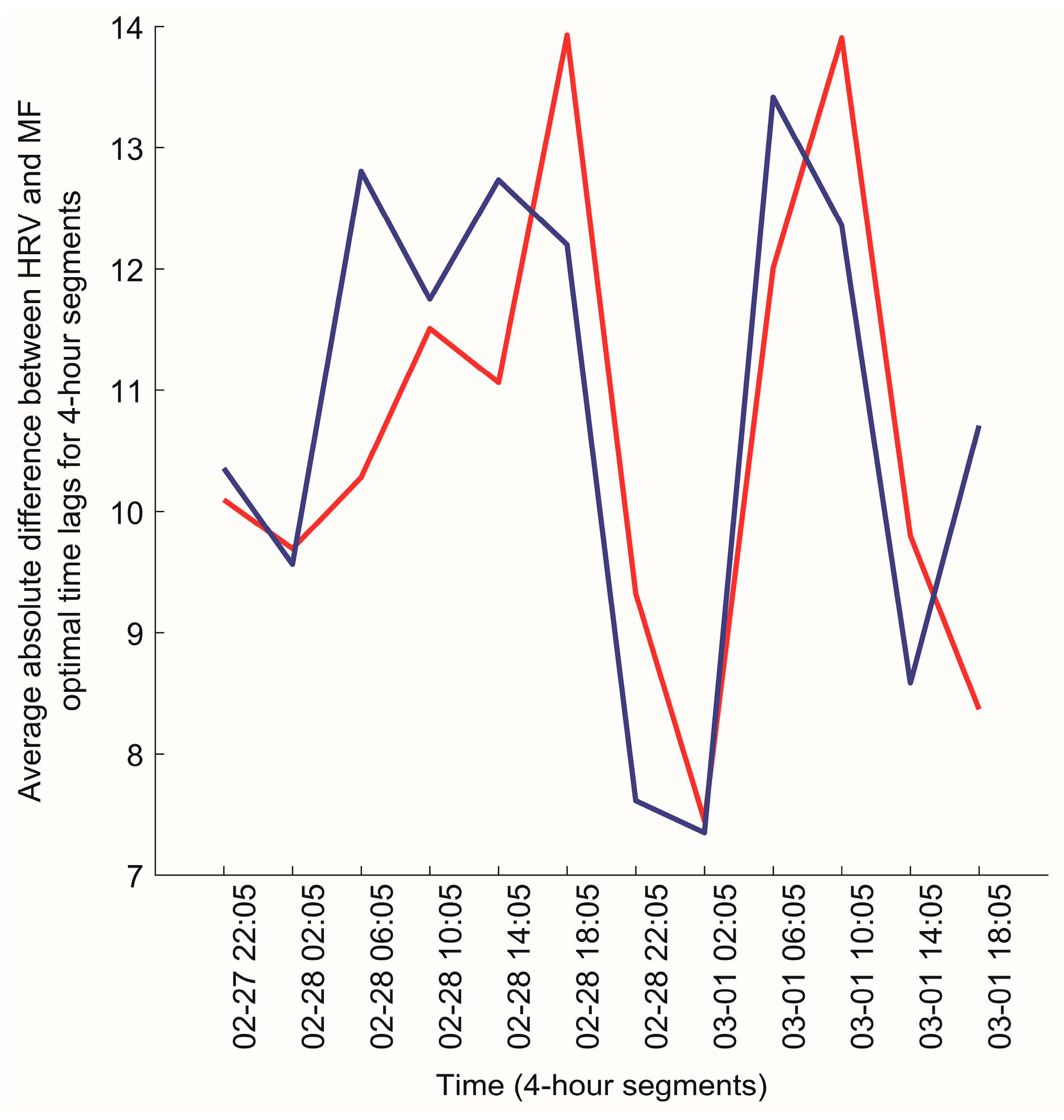
- Calculate the mean absolute difference between optimal time lags for each segment. The obtained vector of mean absolute differences is defined as a measure representing the geometrical synchronization between data signals .
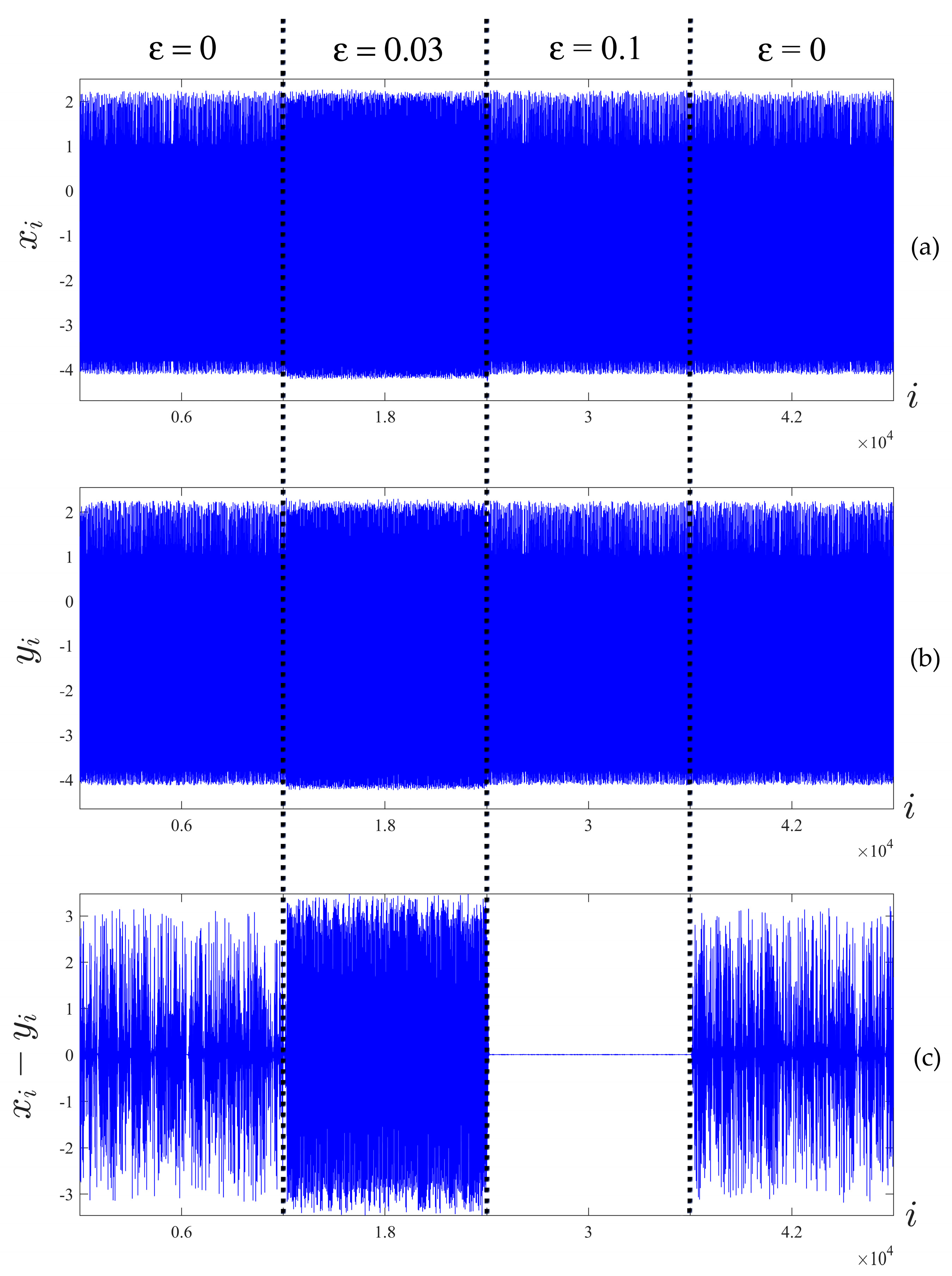
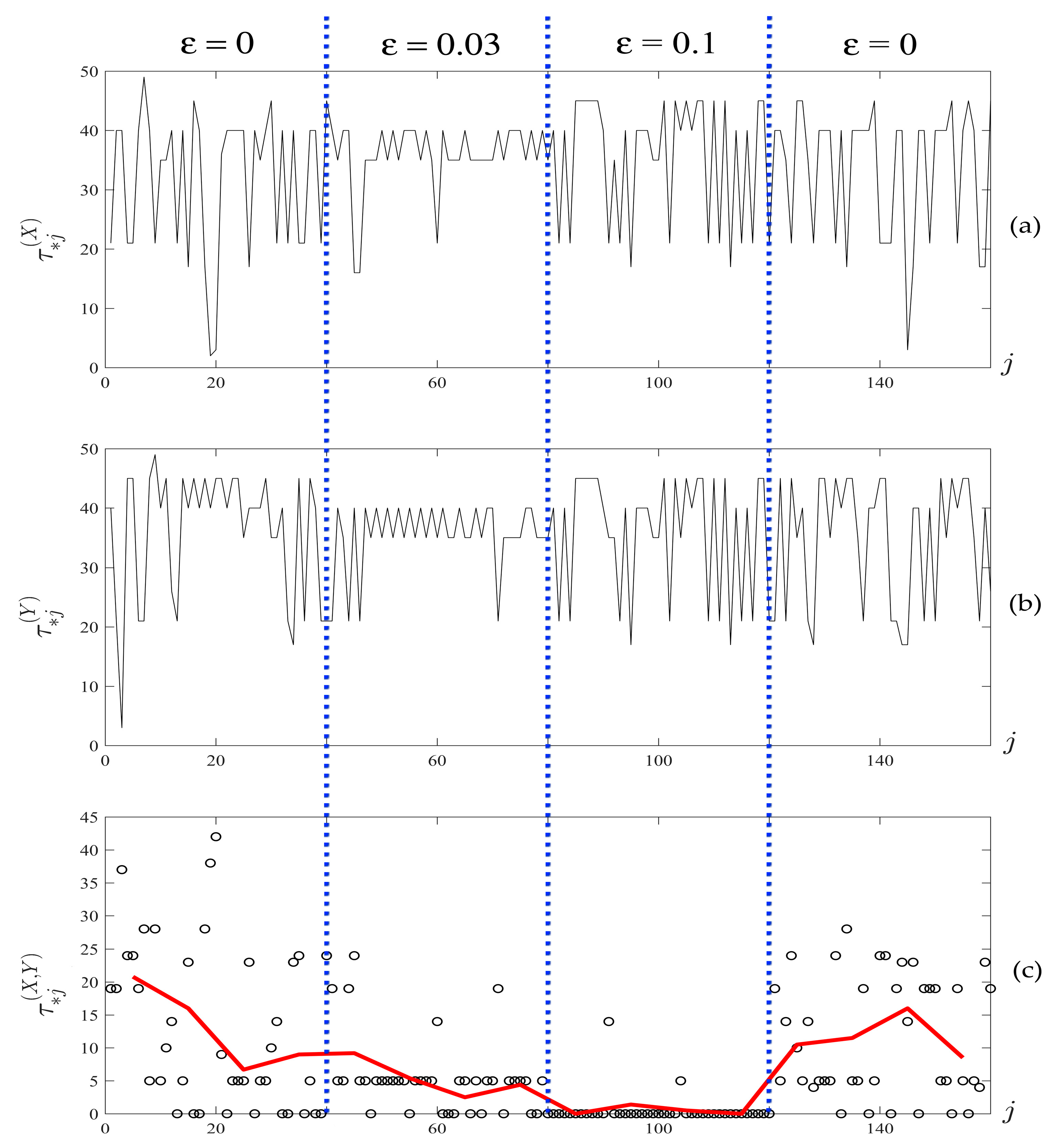
2.5.4. Computational Validation of the Geometrical Synchronization Algorithm
2.6. Clusterization of Multivariate Time Series Based and Their Synchronization with a Master Time Series
- (1)
- Compute the vector of mean absolute differences , describing the relationship between and as described in Algorithm C, for each .
- (2)
- Calculate the Euclidean distance (the measure used to estimate the geometrical similarity of two data vectors) which represents the similarity between all data signals, using the following formula:The above equation yields the symmetric matrix of Euclidean distances.
- (3)
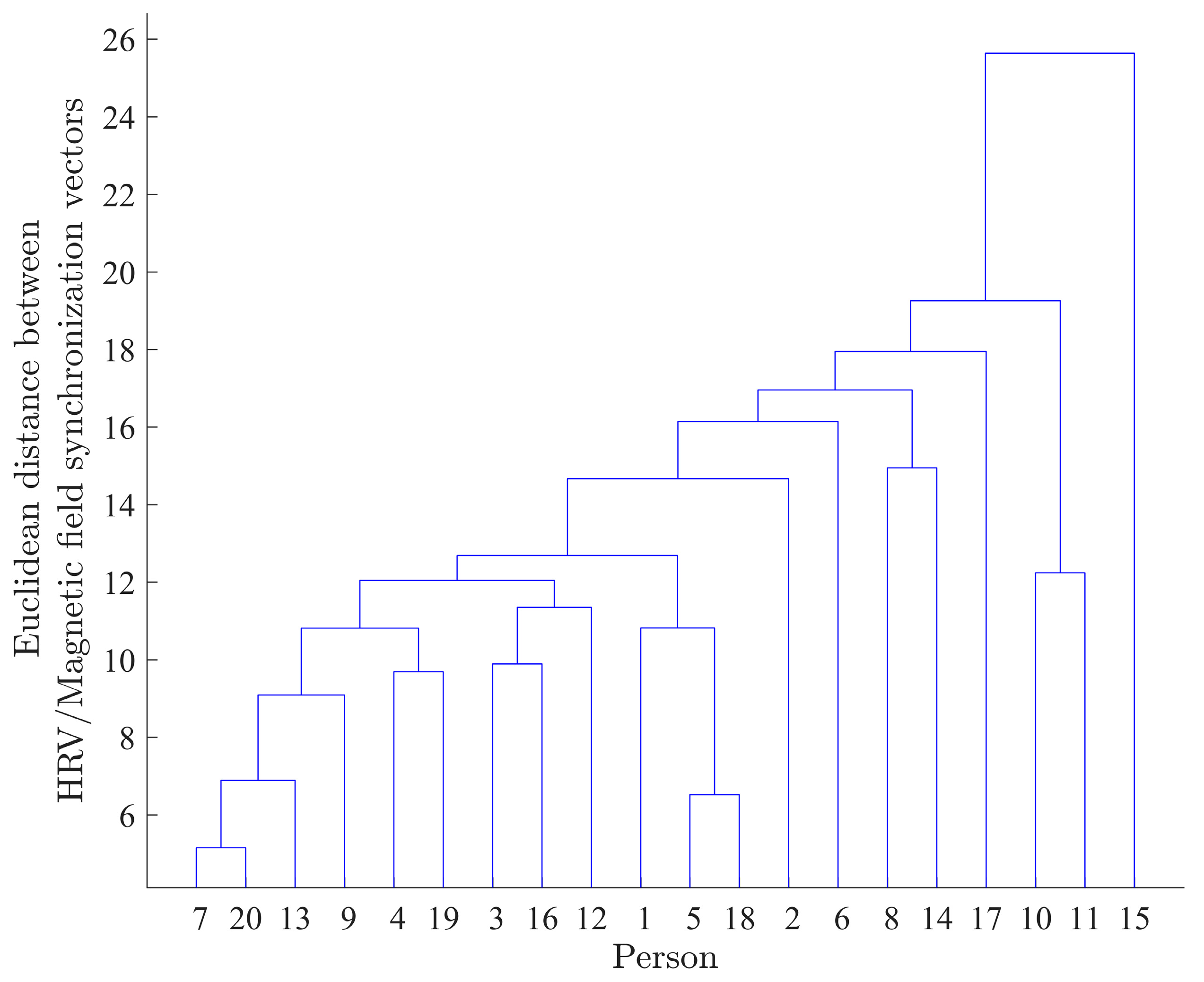
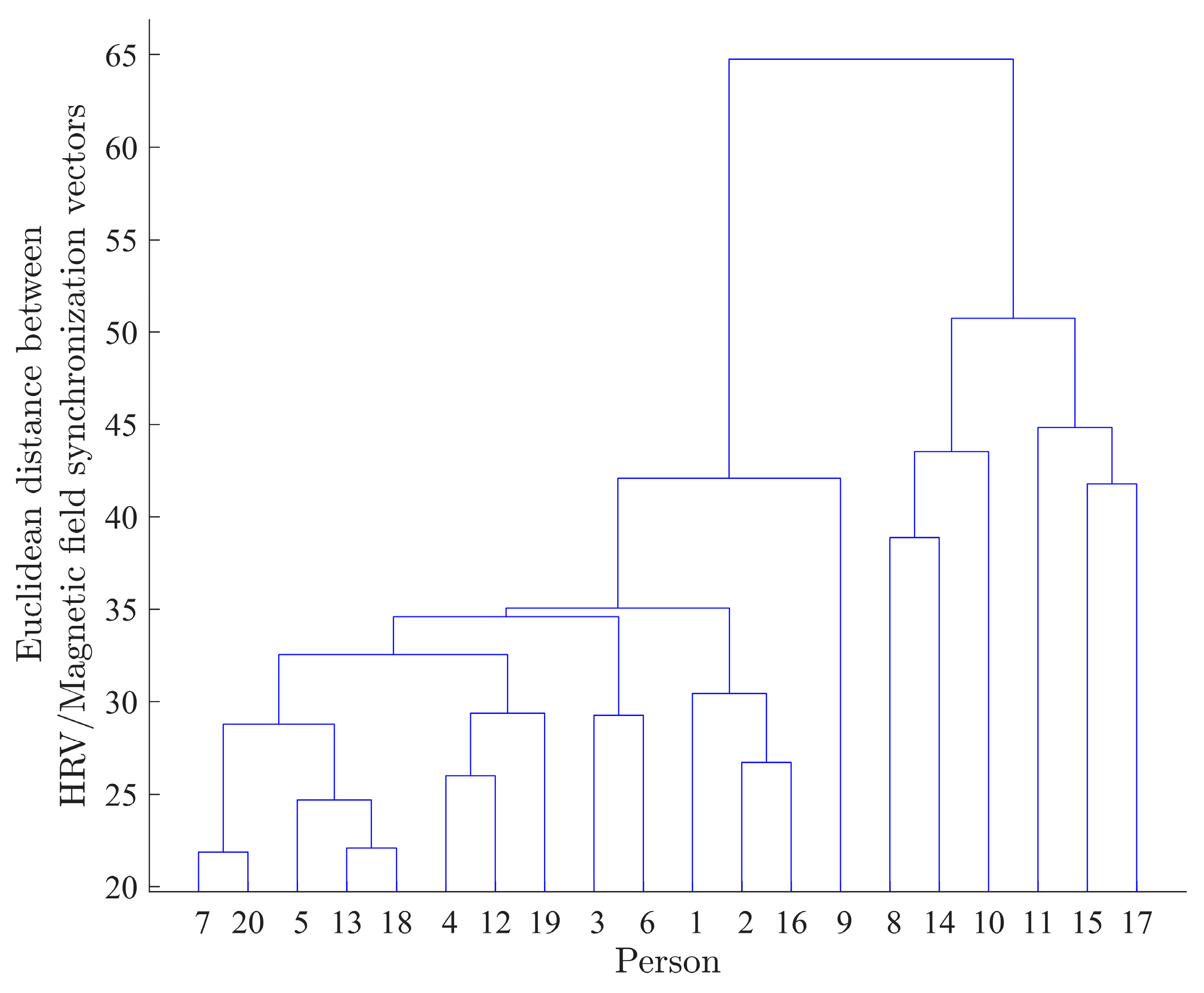
- Construct a dendrogram plot (UPGMA) [37] using the obtained matrix. The main goal of the dendrogram is to identify the clusters of similar time series, i.e., the clustering process involves grouping the analyzed time series based on the similarity of the slower rhythm dynamics of their synchronization with master time series .
3. Results
3.1. The Application of the New Analysis Technique on HRV and Magnetic Field Data
3.1.1. Obtaining the Power of Local Magnetic Field during the Experiment
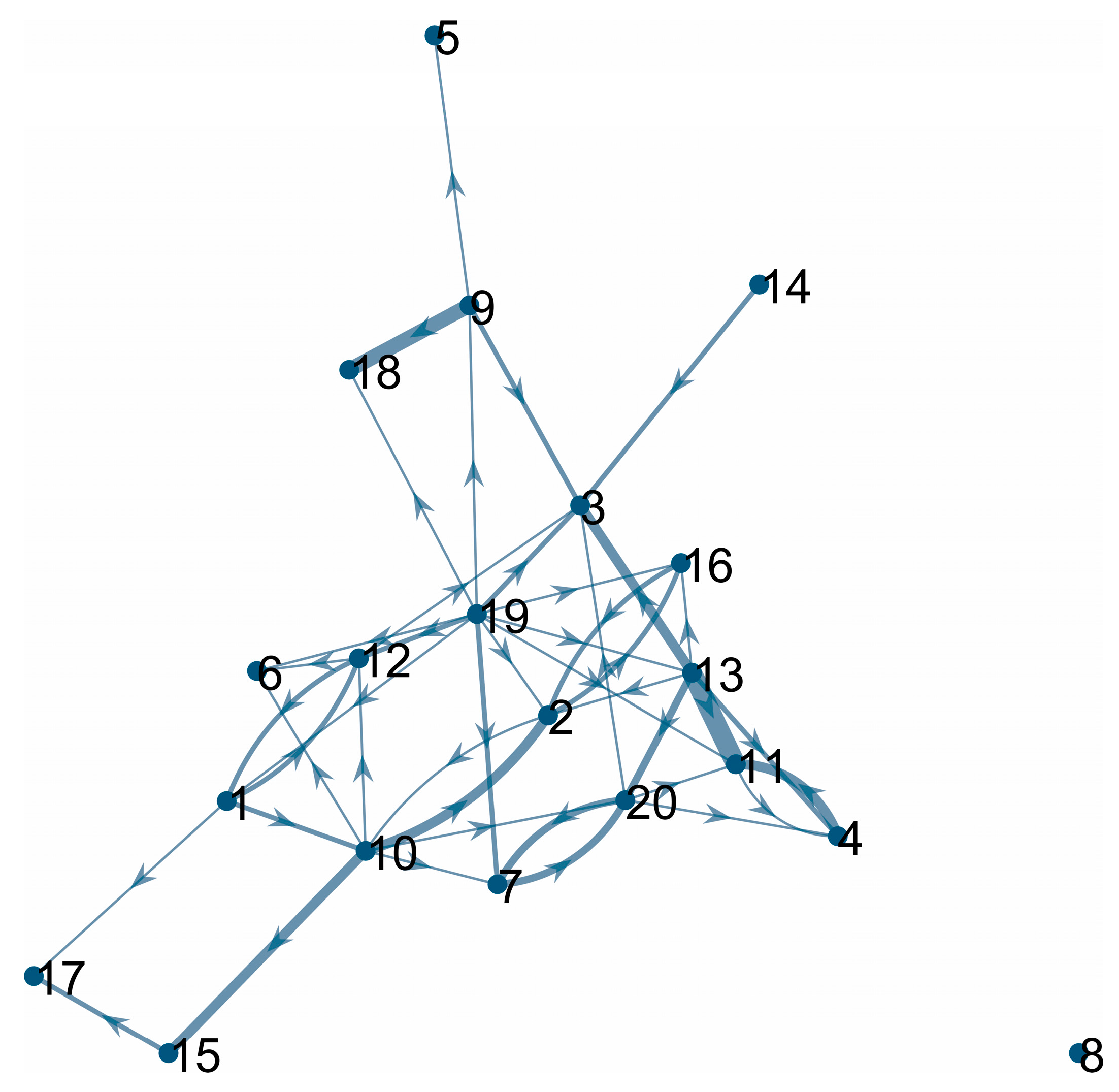
3.1.2. Identification of Clusters in the Groups Based on the Similarity/Synchronization between Participants’ HRV and Magnetic Field Activity
- (1)
- One of the steps of Algorithm C is splitting the participants’ HRV and local magnetic field power time series into segments. The standard length of analysis for HRV is five minutes [38]. Thus, inter-beat (RR) interval and magnetometer data was split into five-minute segments for analysis. Note that since HRV data consists of time intervals between each pair of heartbeats, the number of samples in the data vectors corresponding to each five-minute segment varies due to changes in the participants heart rate and other factors that influence HRV, such as stress and emotional states [39]. Since the power of the local magnetic field was computed for one-second time intervals, the resulting five-minute segments consisted of the same number of elements (300 data points). However, the difference in the size of the segments of HRV and the power of the local magnetic field time series did not impact the overall result of the study, since all of the segments represented the same concurrent five-minute time intervals.
- (2)
- We selected the number of slices in Algorithm B to be 60 because it was empirically observed that a higher number would result in some empty slices.
- (3)
- The maximal value of in Algorithm B was set to 50. Higher values of would generate too short trajectory matrices, because the five-minute segments consisted of approximately 300 elements.
- (4)
- The value of the parameter in Algorithm C, used for identification of slow dynamics of the synchronization between the two time series, was set to 48. This corresponded to a four-hour averaging of the difference of the optimal time lags. It was observed that this value of produced the most meaningful averaging.
- (5)
- As noted in Section 3.2 the magnetometer data contained one minute-long periods of missing data at the end of each hour. Since these periods in the time series did not contain any information, it was necessary to remove those periods in such a way that would not disrupt the timing between the HRV and magnetic field time series. The solution we implemented was to remove the missing data segments from both the five-minute magnetometer data and from the five-minute RR interval series. Since the cropped series obtained after this procedure fully defined the five-minute series, they were used in the data reduction step.
3.2. The Relation between Synchnorization Results and the Psychological Interactions between Participants
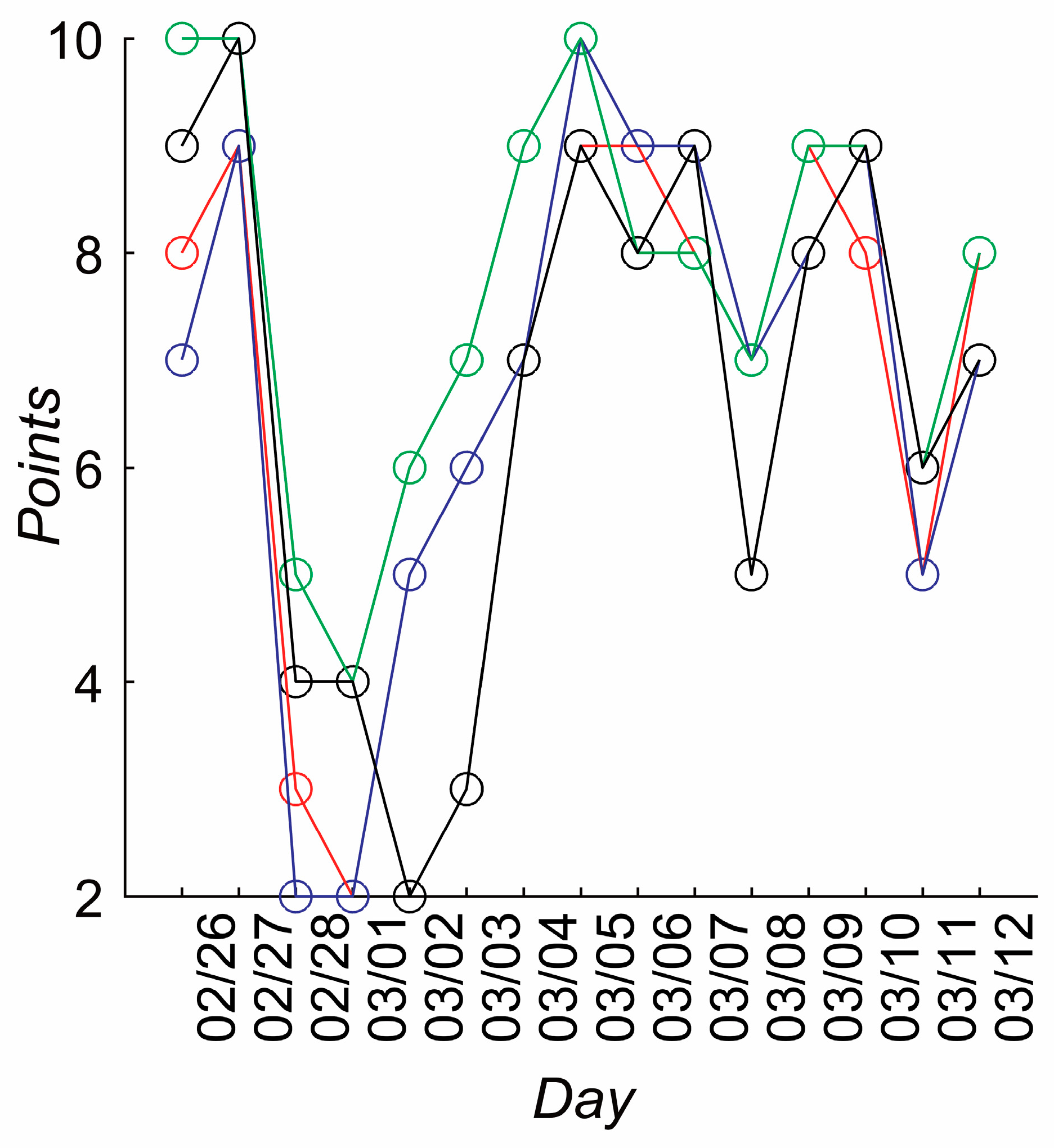
3.2.1. Psychological Survey Data
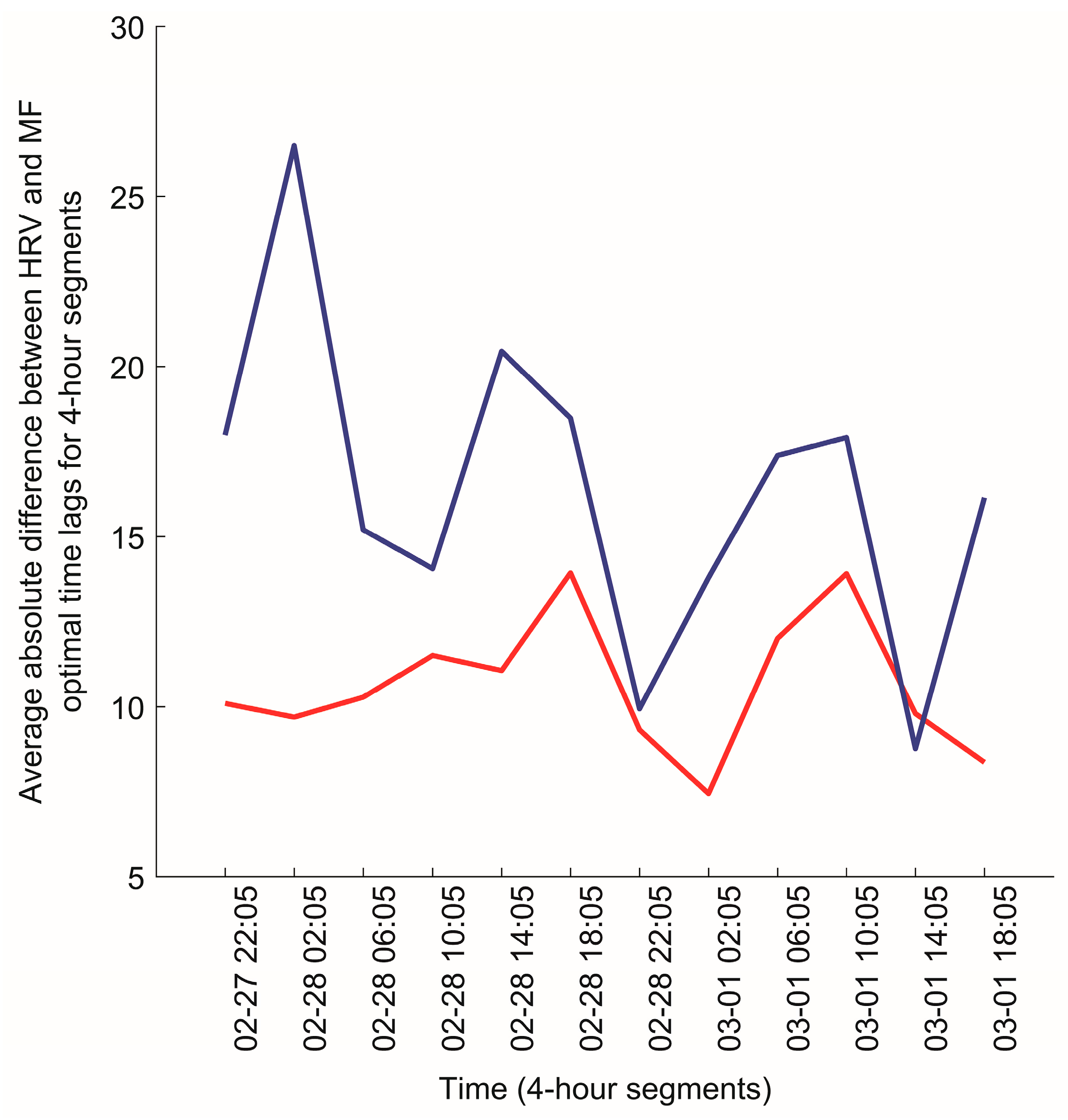
3.2.2. Comparison of Survey Data and the HRV/Magnetic Field Synchronization Results
4. Discussion
5. Conclusions
Supplementary Materials
Acknowledgments
Author Contributions
Conflicts of Interest
Abbreviations
| EEG | Electroencephalogram |
| HRV | Heart rate variability |
| IBI | Inter-beat-interval |
| Pc | pulsations continuous |
| Pi | pulsations irregular |
References
- Otsuka, K.; Cornelissen, G.; Norboo, T.; Takasugi, E.; Halberg, F. Chronomics and “glocal” (combined global and local) assessment of human life. Progress Theor. Phys. Suppl. 2008, 173, 134–152. [Google Scholar] [CrossRef]
- Dimitrova, S.; Stoilova, I.; Cholakov, I. Influence of local geomagnetic storms on arterial blood pressure. Bioelectromagnetics 2004, 25, 408–414. [Google Scholar] [CrossRef] [PubMed]
- Hamer, J.R. Biological entrainment of the human brain by low frequency radiation. Northrop Space Labs 1965, 36, 65–199. [Google Scholar]
- Oraevskii, V.N.; Breus, T.K.; Baevskii, R.M.; Rapoport, S.I.; Petrov, V.M.; Barsukova, Z.V.; Gurfinkel’, I.; Rogoza, A.T. Effect of geomagnetic activity on the functional status of the body. Biofizika 1998, 43, 819–826. [Google Scholar] [PubMed]
- Pobachenko, S.V.; Kolesnik, A.G.; Borodin, A.S.; Kalyuzhin, V.V. The contigency of parameters of human encephalograms and schumann resonance electromagnetic fields revealed in monitoring studies. Complex. Syst. Biophys. 2006, 51, 480–483. [Google Scholar]
- Rapoport, S.I.; Malinovskaia, N.K.; Oraevskii, V.N.; Komarov, F.I.; Nosovskii, A.M.; Vetterberg, L. Effects of disturbances of natural magnetic field of the earth on melatonin production in patients with coronary heart disease. Klin. Med. (Mosk.) 1997, 75, 24–26. [Google Scholar] [PubMed]
- Cornélissen, G.; Halberg, F.; Breus, T.; Syutkina, E.V.; Baevsky, R.; Weydahl, A.; Watanabe, Y.; Otsuka, K.; Siegelova, J.; Fiser, B. Non-photic solar associations of heart rate variability and myocardial infarction. J. Atmos. Sol. Terr. Phys. 2002, 64, 707–720. [Google Scholar] [CrossRef]
- Cornelissen, G.; McCraty, R.; Atkinson, M.; Halberg, F. Gender Differences in Circadian and Extra-Circadian Aspects of Heart Rate Variability (HRV); 1st International Workshop of The TsimTsoum Institute: Krakow, Poland, 2010; pp. 26–27. [Google Scholar]
- Giannaropoulou, E.; Papailiou, M.; Mavromichalaki, H.; Gigolashvili, M.; Tvildiani, L.; Janashia, K.; Preka-Papadema, P.; Papadima, T. A study on the various types of arrhythmias in relation to the polarity reversal of the solar magnetic field. Nat. Hazards 2014, 70, 1575–1587. [Google Scholar] [CrossRef]
- Mavromichalaki, H.; Papailiou, M.; Dimitrova, S.; Babayev, E.; Loucas, P. Space weather hazards and their impact on human cardio-health state parameters on earth. Nat. Hazards 2012, 64, 1447–1459. [Google Scholar] [CrossRef]
- Papailiou, M.; Mavromichalaki, H.; Kudela, K.; Stetiarova, J.; Dimitrova, S. Effect of geomagnetic disturbances on physiological parameters: An investigation on aviators. Adv. Space Res. 2011, 48, 1545–1550. [Google Scholar] [CrossRef]
- Shaffer, F.; McCraty, R.; Zerr, C. A healthy heart is not a metronome: An integrative review of the heart’s anatomy and heart rate variability. Front. Psychol. 2014, 5, 1040. [Google Scholar] [CrossRef] [PubMed]
- Cernouss, S.; Vinogradov, A.; Vlassova, E. Geophysical hazard for human health in the circumpolar auroral belt: Evidence of a relationship between heart rate variation and electromagnetic disturbances. Nat. Hazards 2001, 23, 121–135. [Google Scholar] [CrossRef]
- Watanabe, Y.; Cornelissen, G.; Halberg, F.; Otsuka, K.; Ohkawa, S.I. Associations by signatures and coherences between the human circulation and helio- and geomagnetic activity. Biomed. Pharmacother. 2001, 55 (Suppl. 1), 76s–83s. [Google Scholar] [CrossRef]
- Dimitrova, S.; Angelov, I.; Petrova, E. Solar and geomagnetic activity effects on heart rate variability. Nat. Hazards 2013, 69, 25–37. [Google Scholar] [CrossRef]
- Otsuka, K.; Cornelissen, G.; Weydahl, A.; Holmeslet, B.; Hansen, T.L.; Shinagawa, M.; Kubo, Y.; Nishimura, Y.; Omori, K.; Yano, S.; et al. Geomagnetic disturbance associated with decrease in heart rate variability in a subarctic area. Biomed. Pharmacother. 2001, 55 (Suppl. 1), 51s–56s. [Google Scholar] [CrossRef]
- Otsuka, K.; Ichimaru, Y.; Cornelissen, G.; Weydahl, A.; Holmeslet, B.; Schwartzkopff, O.; Halberg, F. In Dynamic analysis of heart rate variability from 7-day holter recordings associated with geomagnetic activity in subarctic area. Comput. Cardiol. 2000. [Google Scholar] [CrossRef]
- Otsuka, K.; Yamanaka, T.; Cornelissen, G.; Breus, T.; Chibisov, S.; Baevsky, R.; Halberg, F.; Siegelova, J.; Fiser, B. Altered chronome of heart rate variability during span of high magnetic activity. Scr. Med. 2000, 73, 111–116. [Google Scholar]
- Gmitrov, J.; Ohkubo, C. Geomagnetic field decreases cardiovascular variability. Electro Magnetobiol. 1999, 18, 291–303. [Google Scholar] [CrossRef]
- Palmer, S.J.; Rycroft, M.J.; Cermack, M. Solar and geomagnetic activity, extremely low frequency magnetic and electric fields and human health at the earth’s surface. Surv. Geophys. 2006, 27, 557–595. [Google Scholar] [CrossRef]
- Southwood, D. Some features of field line resonances in the magnetosphere. Planet. Space Sci. 1974, 22, 483–491. [Google Scholar] [CrossRef]
- Heacock, R. Two subtypes of type pi micropulsations. J. Geophys. Res. 1967, 72, 3905–3917. [Google Scholar] [CrossRef]
- Alfvén, H. Cosmical. Electrodynamics; Oxford University Press: Oxford, UK, 1963. [Google Scholar]
- McPherron, R.L. Magnetic pulsations: Their sources and relation to solar wind and geomagnetic activity. Surv. Geophys. 2005, 26, 545–592. [Google Scholar] [CrossRef]
- Kleimenova, N.; Kozyreva, O. Daytime quasiperiodic geomagnetic pulsations during the recovery phase of the strong magnetic storm of 15 May 2005. Geomagn. Aeron. 2007, 47, 580–587. [Google Scholar] [CrossRef]
- Appelhans, B.M.; Luecken, L.J. Heart rate variability as an index of regulated emotional responding. Rev. Gen. Psychol. 2006, 10, 229–240. [Google Scholar] [CrossRef]
- Butler, E.A.; Wilhelm, F.H.; Gross, J.J. Respiratory sinus arrhythmia, emotion, and emotion regulation during social interaction. Psychophysiology 2006, 43, 612–622. [Google Scholar] [CrossRef] [PubMed]
- Doronin, V.N.; Parfentev, V.A.; Tleulin, S.Z.; Namvar, R.A.; Somsikov, V.M.; Drobzhev, V.I.; Chemeris, A.V. Effect of variations of the geomagnetic field and solar activity on human physiological indicators. Biofizika 1998, 43, 647–653. [Google Scholar] [PubMed]
- Zenchenko, T.; Medvedeva, A.; Khorseva, N.; Breus, T. Synchronization of human heart-rate indicators and geomagnetic field variations in the frequency range of 0.5–3.0 mHZ. Izvestiya Atmos. Ocean. Phys. 2014, 50, 736–744. [Google Scholar] [CrossRef]
- McCraty, R.; Atkinson, M.; Stolc, V.; Alabdulgader, A.A.; Vainoras, A.; Ragulskis, M. Synchronization of human autonomic nervous system rhythms with geomagnetic activity in human subjects. Int. J. Environ. Res. Public Health 2017, 14, 770. [Google Scholar] [CrossRef] [PubMed]
- Alabdulgade, A.; Maccraty, R.; Atkinson, M.; Vainoras, A.; Berškienė, K.; Mauricienė, V.; Navickas, Z.; Šmidtaitė, R.; Landauskas, M.; Daunoravičienė, A. Human heart rhythm sensitivity to earth local magnetic field fluctuations. J. Vibroeng. 2015, 17, 3271–3278. [Google Scholar]
- McCraty, R.; Deyhle, A. The global coherence initative: Investigating the dynamic relationship between people and earth’s energetic systems. In Bioelectromagnetic and Subtle Energy Medicine, 2nd ed.; Rosch, P.J., Ed.; CRC Press: Boca Raton, FL, USA, 2015. [Google Scholar]
- Heartmath Institute: Live Magnetometer Data. Available online: https://www.heartmath.org/research/global-coherence/gcms-live-data/ (accessed on 30 August 2017).
- Sauer, T.; Yorke, J.A.; Casdagli, M. Embedology. J. Stat.Phys. 1991, 65, 579–616. [Google Scholar] [CrossRef]
- Ragulskis, M.; Lukoseviciute, K. Non-uniform attractor embedding for time series forecasting by fuzzy inference systems. Neurocomputing 2009, 72, 2618–2626. [Google Scholar] [CrossRef]
- Hilborn, R.C. Chaos and Nonlinear Dynamics: An Introduction for Scientists and Engineers; Oxford University Press: Oxford, UK, 2000. [Google Scholar]
- Sneath, P.H.A.; Sokal, R.R. Numerical Taxonomy. The Principles and Practice of Numerical Classification; W H Freeman & Co.: San Francisco, CA, USA, 1973; p. 573. [Google Scholar]
- Camm, A.J.; Malik, M.; Bigger, J.T.; Breithardt, G.; Cerutti, S.; Cohen, R.J.; Singer, D.H. Heart rate variability standards of measurement, physiological interpretation, and clinical use. Task force of the European society of cardiology and the North American society of pacing and electrophysiology. Circulation 1996, 93, 1043–1065. [Google Scholar]
- McCraty, R.; Atkinson, M.; Tiller, W.A.; Rein, G.; Watkins, A.D. The effects of emotions on short-term power spectrum analysis of heart rate variability. Am. J. Cardiol. 1995, 76, 1089–1093. [Google Scholar] [CrossRef]


| N | 1 | 2 | 3 | 4 | 5 | 6 | 7 | 8 | 9 | 10 | 11 | 12 | 13 | 14 | 15 | 16 | 17 | 18 | 19 | 20 |
|---|---|---|---|---|---|---|---|---|---|---|---|---|---|---|---|---|---|---|---|---|
| 1 | −1 | −1 | 2 | 2 | 1 | −1 | ||||||||||||||
| 2 | 1 | 2 | ||||||||||||||||||
| 3 | ||||||||||||||||||||
| 4 | −1 | 4 | ||||||||||||||||||
| 5 | ||||||||||||||||||||
| 6 | ||||||||||||||||||||
| 7 | 3 | |||||||||||||||||||
| 8 | ||||||||||||||||||||
| 9 | 2 | 1 | 6 | |||||||||||||||||
| 10 | 4 | 1 | 1 | 1 | 4 | 1 | ||||||||||||||
| 11 | 1 | |||||||||||||||||||
| 12 | 2 | 1 | 1 | −1 | ||||||||||||||||
| 13 | 1 | 4 | 2 | 8 | 1 | 3 | ||||||||||||||
| 14 | 2 | |||||||||||||||||||
| 15 | 2 | |||||||||||||||||||
| 16 | 2 | |||||||||||||||||||
| 17 | ||||||||||||||||||||
| 18 | ||||||||||||||||||||
| 19 | 1 | 1 | 2 | 1 | 2 | 1 | 1 | 2 | 1 | 1 | 1 | |||||||||
| 20 | 1 | 1 | 3 | 1 |
© 2017 by the authors. Licensee MDPI, Basel, Switzerland. This article is an open access article distributed under the terms and conditions of the Creative Commons Attribution (CC BY) license (http://creativecommons.org/licenses/by/4.0/).
Share and Cite
Timofejeva, I.; McCraty, R.; Atkinson, M.; Joffe, R.; Vainoras, A.; Alabdulgader, A.A.; Ragulskis, M. Identification of a Group’s Physiological Synchronization with Earth’s Magnetic Field. Int. J. Environ. Res. Public Health 2017, 14, 998. https://doi.org/10.3390/ijerph14090998
Timofejeva I, McCraty R, Atkinson M, Joffe R, Vainoras A, Alabdulgader AA, Ragulskis M. Identification of a Group’s Physiological Synchronization with Earth’s Magnetic Field. International Journal of Environmental Research and Public Health. 2017; 14(9):998. https://doi.org/10.3390/ijerph14090998
Chicago/Turabian StyleTimofejeva, Inga, Rollin McCraty, Mike Atkinson, Roza Joffe, Alfonsas Vainoras, Abdullah A. Alabdulgader, and Minvydas Ragulskis. 2017. "Identification of a Group’s Physiological Synchronization with Earth’s Magnetic Field" International Journal of Environmental Research and Public Health 14, no. 9: 998. https://doi.org/10.3390/ijerph14090998