1. Introduction
Hypertension is a common chronic disease and a main risk factor for cardiovascular and cerebrovascular diseases. According to the 2013 World Health Organization (WHO) report, 9.4 million people were dying of complications due to hypertension. The continuous worldwide high prevalence of hypertension, especially in low- and middle-income countries, severely consumes medical and social resources, placing a heavy burden on families and countries. Using data from the 2010 National Population Census, the total number of people with hypertension in China was approximately 270 million. The Survey on the Status of Nutrition and Health of the Chinese People in 2012 showed that 25.2% of adults aged 18 or older in China had hypertension [
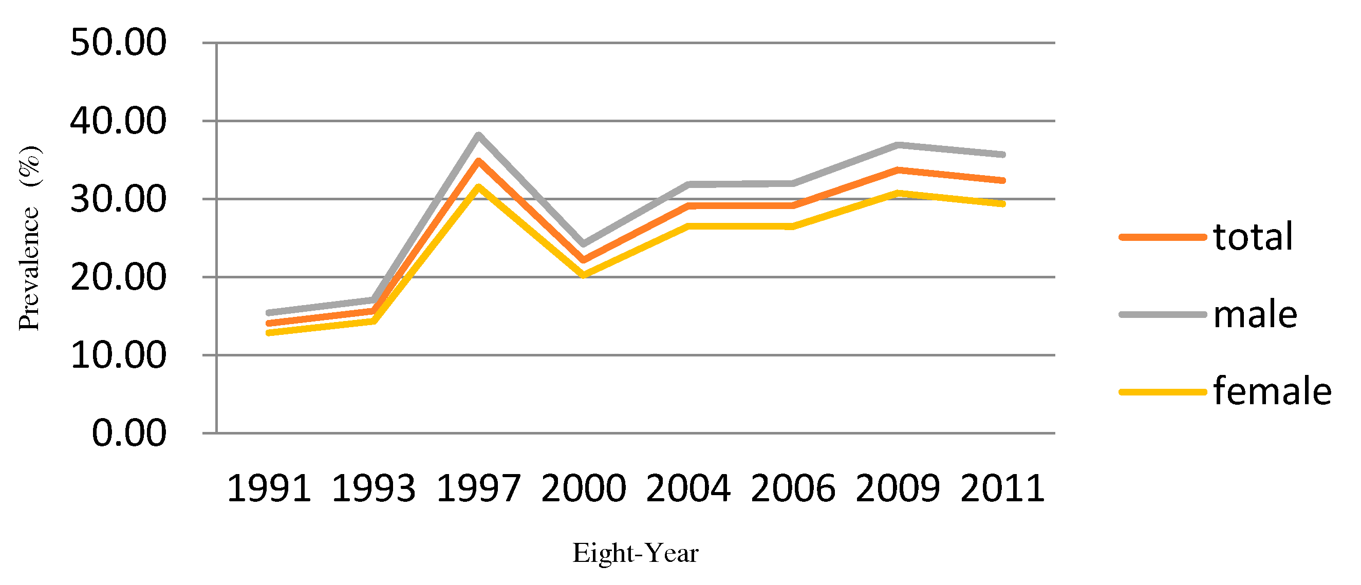
1]. Inhabitants in China aged 18 or older have been reported to have a hypertension prevalence of 33.5%, with the rate in urban areas higher than that of rural areas (34.7% vs. 32.9%); the prevalence in men was higher than that in women (35.1% vs. 31.8%), and the prevalence in Eastern China, central China, and Western China were 36.2%, 34.1%, and 28.8%, respectively, in 2010 [
2]. This indicated that the prevalence of hypertension in China has significant spatio-temporal variations in addition to being continuously high, providing a new direction for research into the risk factors for hypertension and its preventive control.
To explore spatial variations of diseases, spatial epidemiology is a systematic branch of epidemiology [
3]. Disease mapping, especially Bayesian disease mapping, is a research hotspot in the field of spatial epidemiology. It visually identifies spatial patterns of disease and presents the results from a spatial perspective [
4]. Furthermore, presenting result on a map can allow the acquisition of an intuitive and perceptual understanding, providing clues for further etiology research. In addition, disease mapping provides a rapid and visualized summary of complicated geographic information, enabling the identification of subtle patterns not visible in tabular presentations [
5]. With advances in computer technology, such as the Markov chain Monte Carlo (MCMC) method, the applications of the Bayesian hierarchical models (BHM) have become increasingly popular due to its flexibility and easy expansion. Gelman acknowledged that BHM is a flexible tool for combining information and the partial pooling of inferences, providing a more objective method for inferences by estimating the parameters of prior distributions from data rather than requesting the data to be specified using subjective information [
6].
The shared components model (SCM) is a widely-used disease mapping method based on the BHM framework. SCM was introduced by Knorr and Best [
7]. SCM has been attracting increasing amounts of attention in the research on Bayesian joint disease mapping of two diseases or multiple diseases. It operates on the basic idea that many diseases share common risk factors, thus the underlying risk variations can be decomposed into shared and disease-specific components. The shared components, also called unobservable covariates, are the common risk factors of multiple diseases, whereas the disease-specific components represent space-varying disease-specific risk factors. SCM was used in many studies, such as for gender correlation of disease risk, sparse data in small areas, errors occurring in covariates, disease risk estimates for data from multiple sources, omission of estimated date, and disability-adjusted life year (DALY) in small areas [
8,
9,
10,
11,
12,
13,
14,
15,
16,
17].
According to these studies, the SCM has become an increasingly popular model for disease mapping due to its flexibility, convenience, and robustness of estimates. However, simultaneously including the spatial and temporal dependence structures in a model is difficult; previous research has mainly focused on spatial analysis. However, these studies were mainly conducted to explore the morbidity or mortality risk of rare diseases, such as cancer, in limited areas, whereas studies on non-rare disease were rarer.
Thus, we tried to incorporate time trends into SCM using Bayesian B-spline fitting. This study explored the hypertension prevalence pattern and the evolution of its relevant factors, in seven provinces in China from 1991 to 2011, according to China Health and Nutrition Survey (CHNS) data. Considering that hypertension is a chronic disease, some lifestyles, such as smoking and drinking alcohol, may have a lagging effect. We performed an overall analysis combining the risk estimate with a population index. As the time span of this study is quite long (20 years), which may generate spatio-temporal interactions, we introduced interactive items into the model with the goal of better exploring the spatio-temporal evolution patterns in hypertension risk, thus providing guidance for spatio-temporal monitoring of diseases and implementing appropriate health policies.
4. Discussion
The high prevalence of hypertension not only affects quality of life but also creates a heavier disease burden for both individuals and society as a whole. To advance the efficiency of disease control, specialists tried to identify the areas with high hypertension prevalence and reveal the hypertension risk factors. Previous research found that gender variations may exist in hypertension prevalence [
24,
25,
26]; however, the research was limited because most of the studies were conducted using traditional statistical methods, such as logistic regression, which do not consider spatial information. Hence, the mixture of lifestyle choices and environmental factors, which might cause the spatial variation in the risk of hypertension, was not effectively revealed. As for this study, SCM was performed to explore regional gender variation in the hypertension risk in seven provinces of China. This paper focused on hypertension, a common disease, and broadened the exiting SCM by adding Bayesian B-spline to fit time-related random components. As a result, these models could be applied to investigate regional and gender variations in hypertension risk, and whether the spatial distribution of hypertension risk is formed by persistence or chance, and to study non-rare diseases to explore risk factors at the regional level.
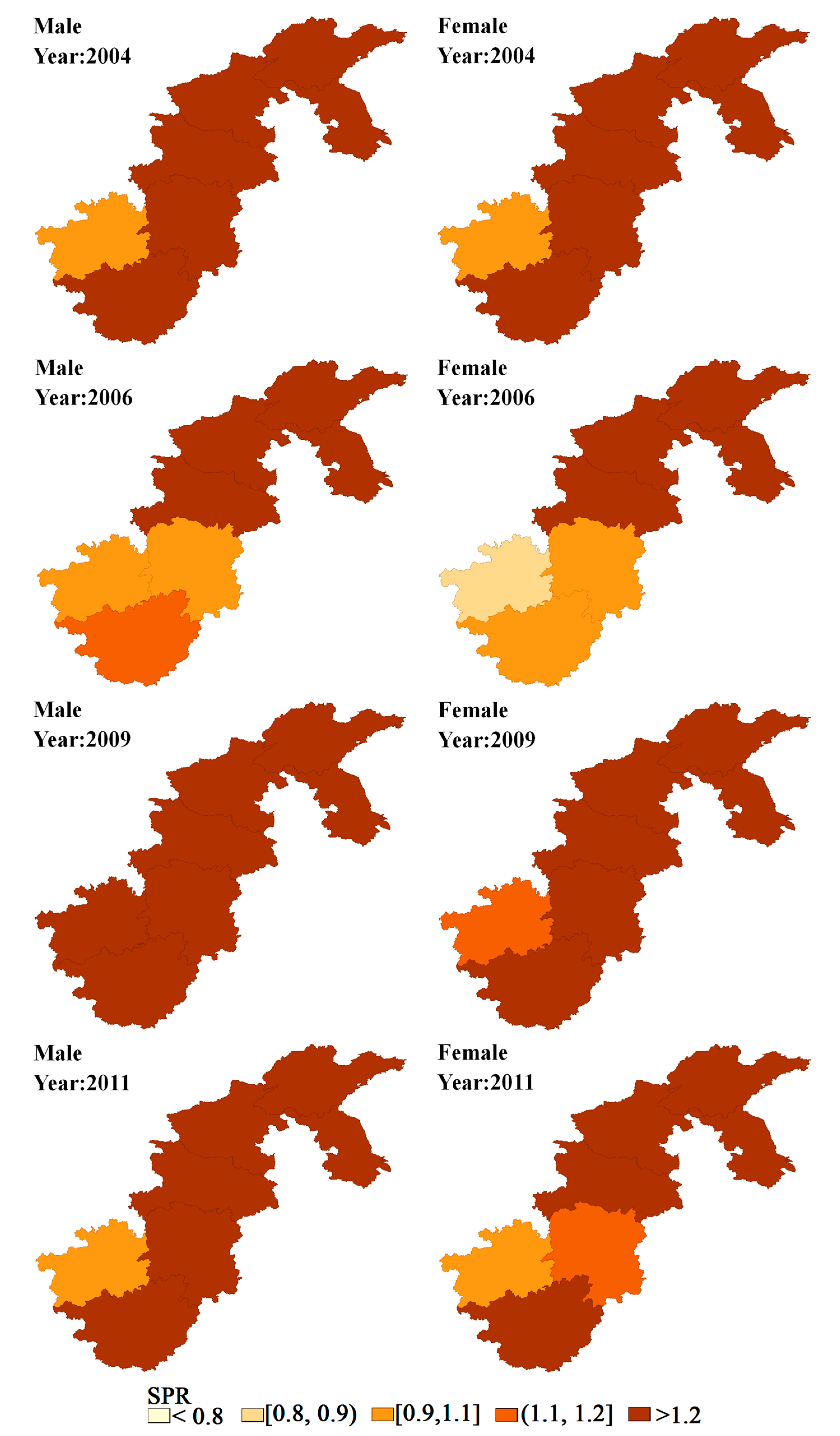
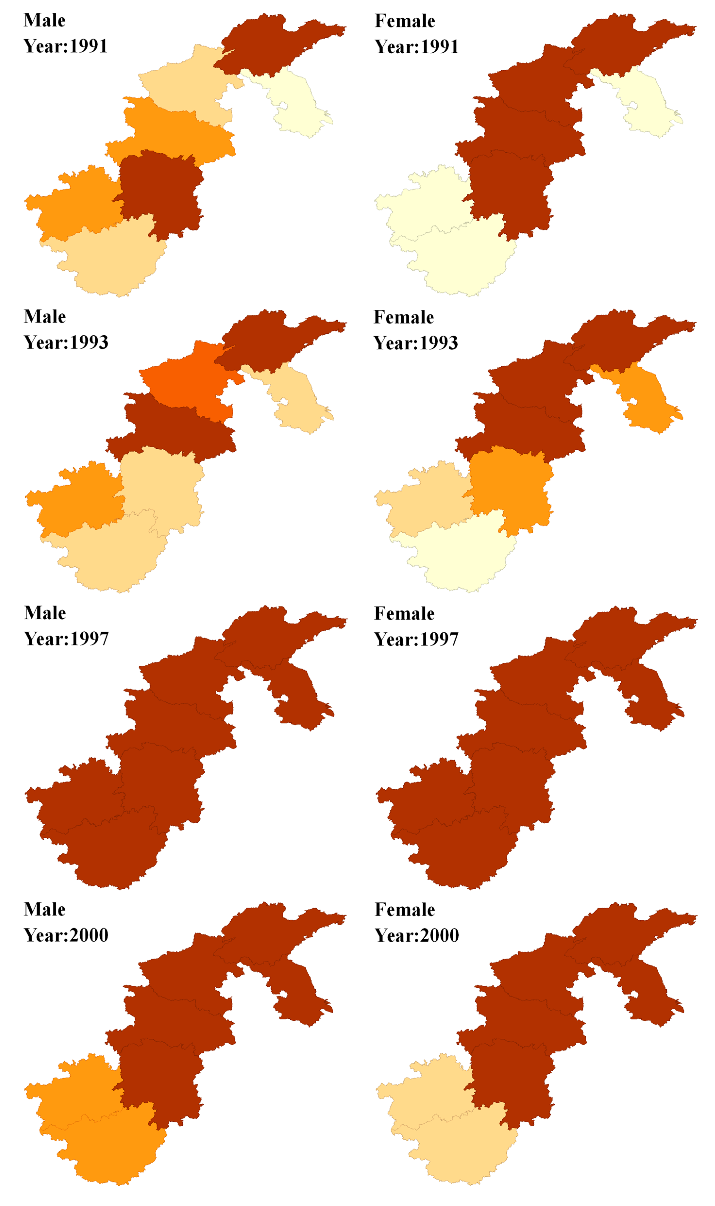
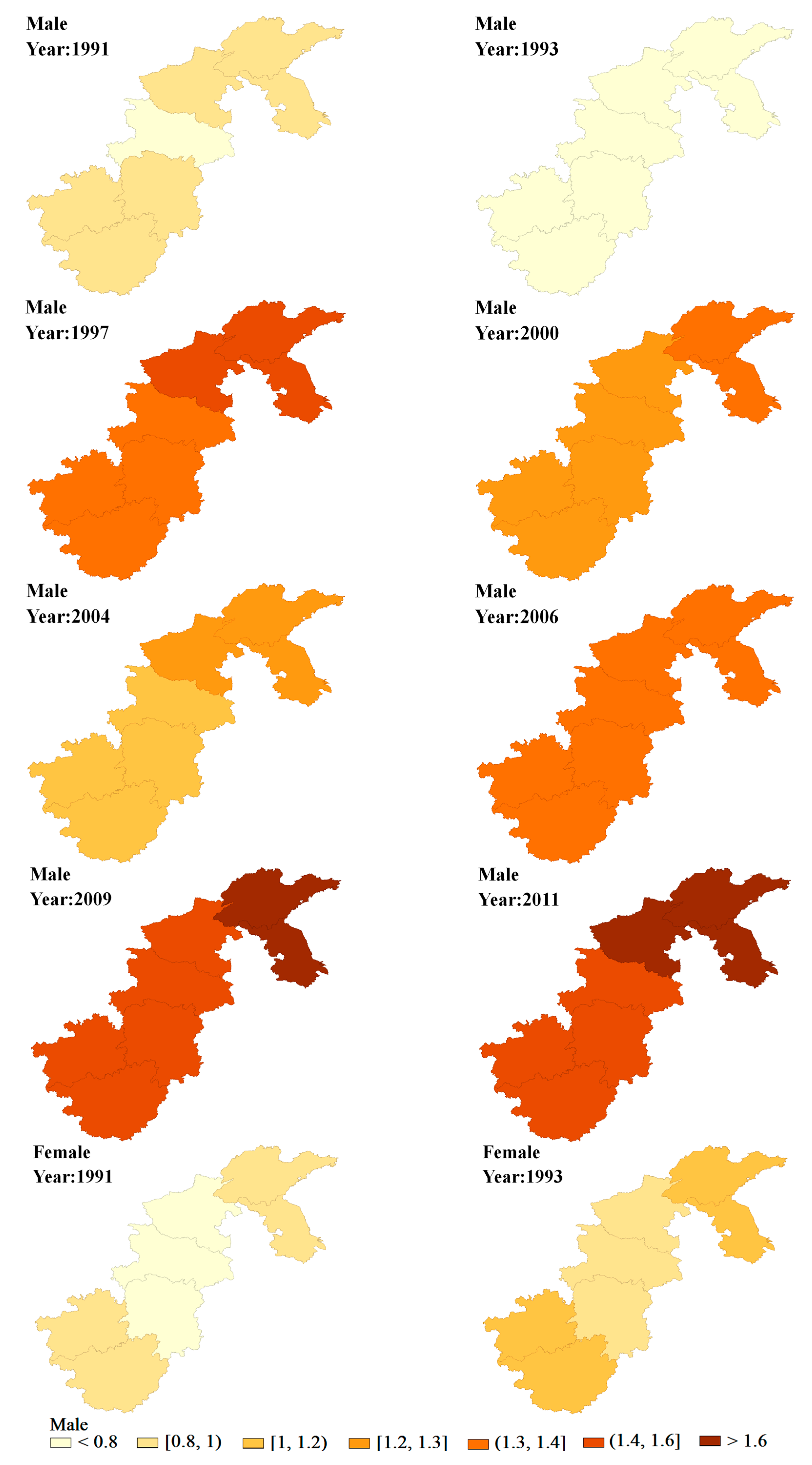
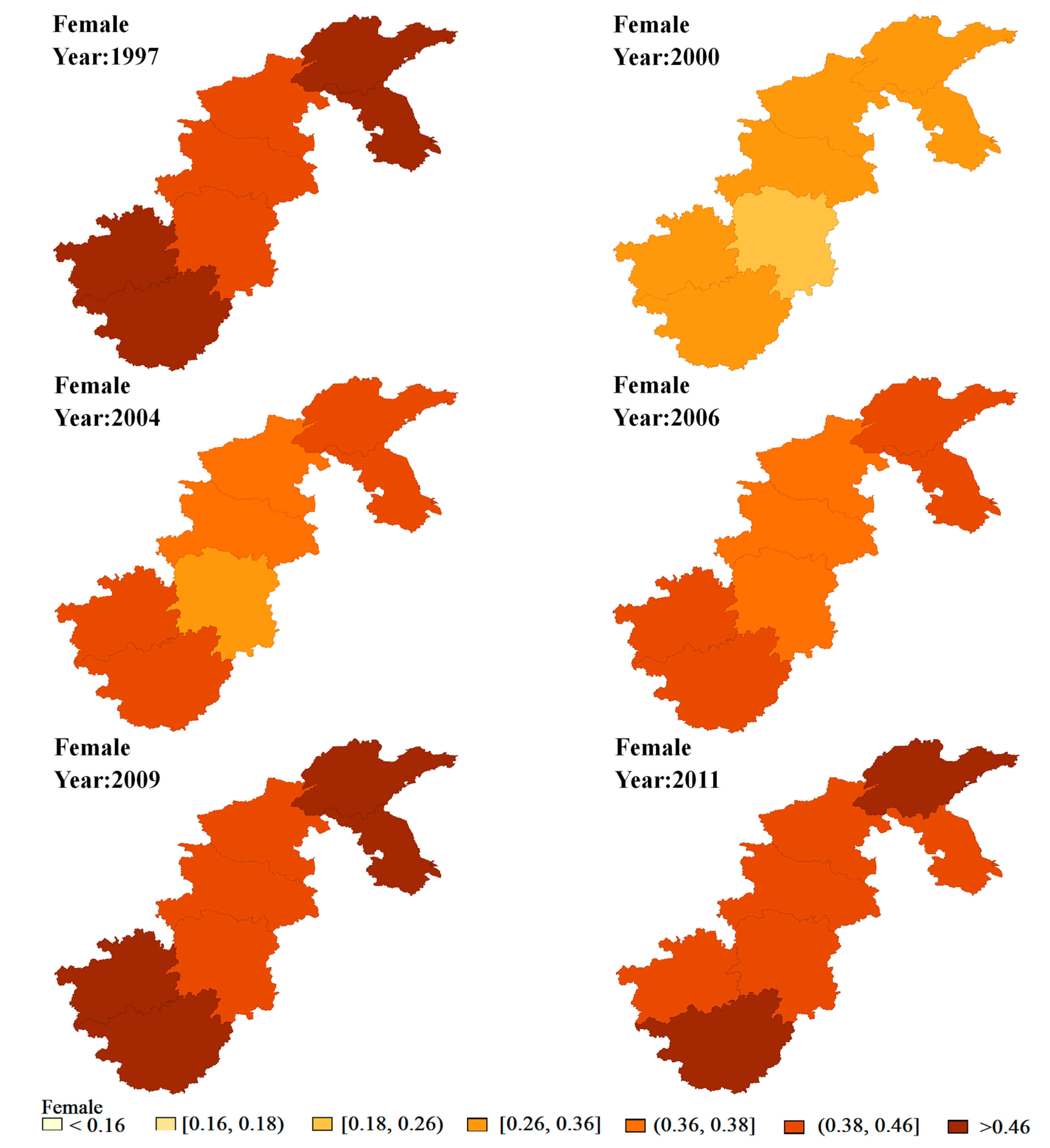
Given the results derived from the spatio-temporal analysis, the spatio-temporal distribution of hypertension exhibited certain spatial clustering. The prevalence was higher in the north, such as in Jiangsu, Shandong and Henan, which was the same as found in previous research [
27]. Moreover, the boundary points of the time trend in the hypertension risk occurred in 1997, 2000, and 2004 for men, whereas it occurred in 1997 and 2004 for women. Before 1997, the hypertension risk for both genders remained low. After that, especially since 2004, the hypertension risk in all seven provinces increased over time, particularly in northern China, in some neighboring provinces, such as Jiangsu, Shandong and Henan. However, in the neighboring provinces, such as Hunan and Guizhou, the hypertension risk remained relatively low. Notably, the hypertension risk in Shandong and Jiangsu province, for men in particular, continuously stood out after 2004, so special attention should be paid to this region for hypertension prevention and control.
Further analysis of the above-mentioned spatial–temporal variations showed that the prevalence of hypertension in provinces like Jiangsu, Shandong, Henan provinces remained relatively high, whereas the rates in Hunan and Guizhou remained at an evidently lower level. Given the fact that the proportions of obesity and alcohol consumption are high in the northern provinces, the above findings may indicate that factors associated with lifestyle, such as obesity [
28,
29] and alcohol consumption [
30], might be the main causes of the increasing hypertension risk in some regions. Furthermore, the inhabitants in provinces with a high hypertension risk prefer foods with stronger flavors in their daily life, and high-salt diets were quite typical. Therefore, high-salt diets might be another important reason for the increasing hypertension risk, verifying most of the research conclusions [
31,
32]. Thus, to reduce the prevalence of hypertension in northern China, some intervention programs aimed at lifestyle choices should be implemented.
To be specific, from 2004 onwards, the hypertension risk for men in Henan remained at a relatively high level. Further analysis found that the smoking rate for men in Henan was considerably higher than that in other provinces prior to 2004, implying that the negative influence of smoking on hypertension might have a time lag of at least 10 years, consistent with previous research [
33,
34].
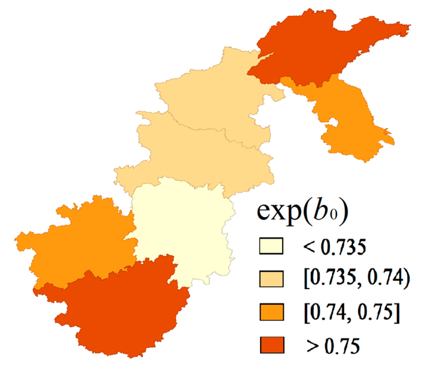
The distribution of
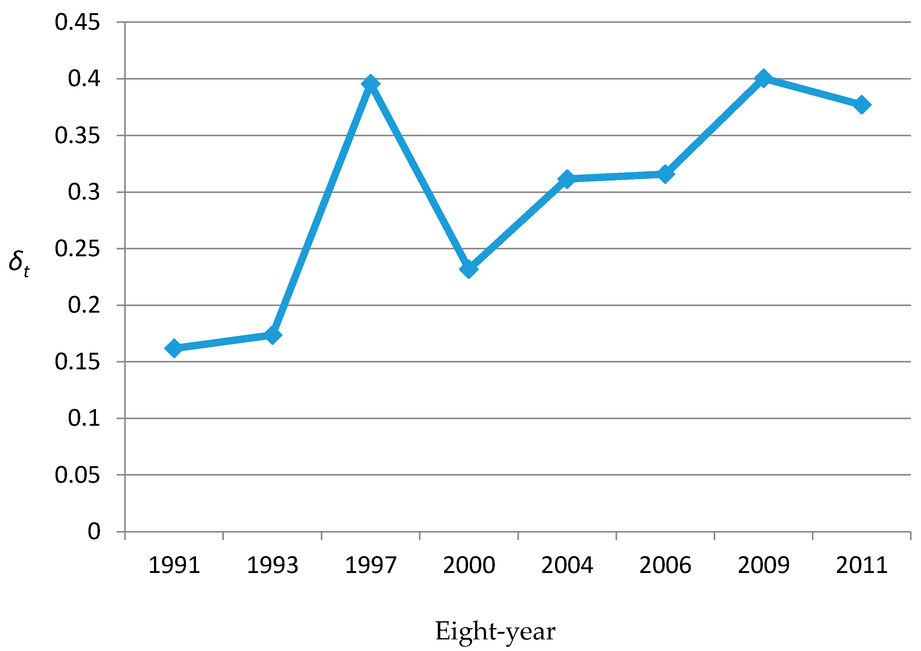
βit indicated that the hypertension risk presented no evident gender variation and remained stable over time after removing the spatio-temporal variations common and specific to both genders. The results of other SCM parameters are shown in
Figure 4 and
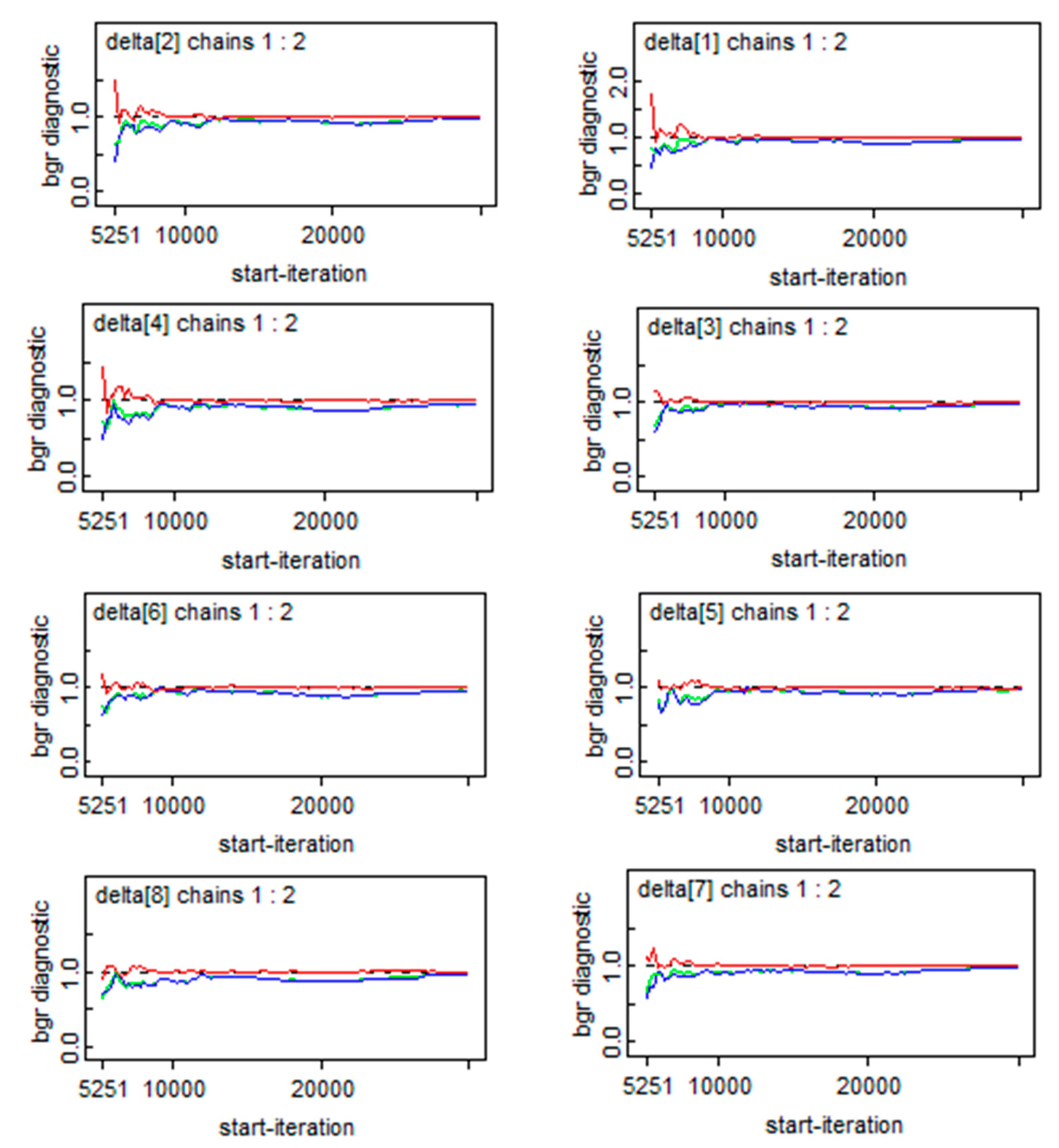
Figure 5. Combining the results of the common components and the corresponding weight (
δ) may suggest that some common unobserved factors, such as atmosphere pollution, dominated the spatio-temporal variations in the risk of hypertension for men and women [
35].
We believe our study will contribute to the medical literature in the following ways: (1) To broaden the existing SCM, Bayesian B-spline was added to fit the time trend so that spatial and temporal information could be simultaneously and effectively incorporated into the model. Therefore, the continuity and contingency patterns of disease risk were clearly shown, providing reliable information for the deeper exploration of disease causes. (2) Our study showed that, though often applied to rare diseases, the SCM can also be applied to non-rare diseases to identify risk factors at the regional level and quantify gender-specific fixed effects [
36].
Limited by time and research conditions, some areas of this study need further study and improvements. Firstly, this study used the province level as the analysis scale, which might lead to considerable uncertainty for the statistical inference of parameters, but data on a finer scale, such as at the city level or the county level, could not be acquired due to some principled requests, such as the privacy of survey data. Secondly, in the spatial analysis of SCM, the commonly-used CAR and Gaussian distribution were assumed for the spatially structured and unstructured random effects, respectively. As a result, this may lead to not fully estimating the impact of some situations, such as different degrees of spatial correlations occurring and extreme values existing in samples on the estimates of disease risk, which is the future direction of this work. Thirdly, in this study, some hypertension risk factors, such as smoking and drinking, were not introduced into the spatio-temporal models as covariates, hence, a deeper explanation for the spatio-temporal variations of risk factors is lacking. However, the increase in complexity may lead to a failure of the identification of the SCM, which restricted our research to some extent.


