Comparative Analysis of GF-1 and HJ-1 Data to Derive the Optimal Scale for Monitoring Heavy Metal Stress in Rice

Abstract
:1. Introduction
2. Study Area and Data
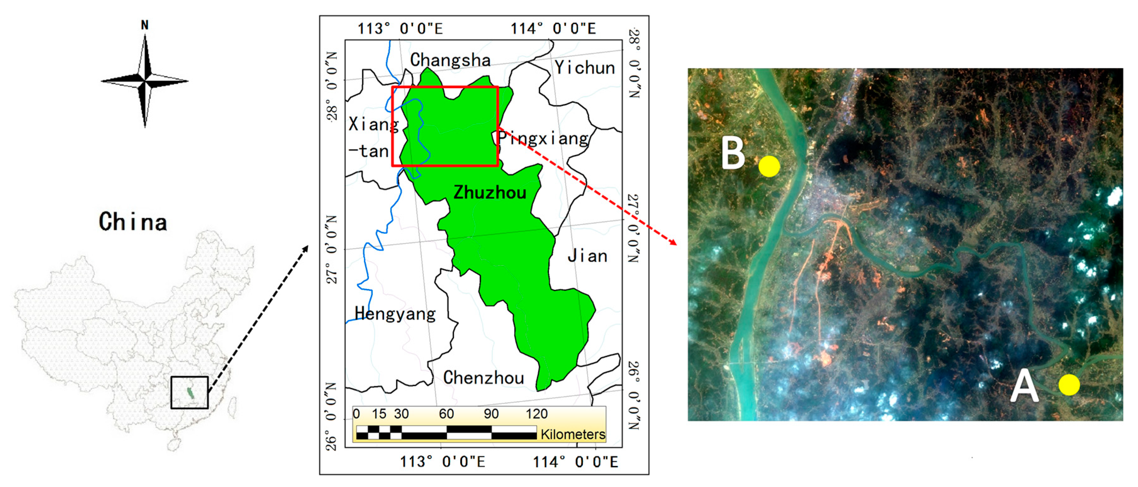
2.1. Study Area
2.2. Remote Sensing Data
2.3. Measured Data
2.4. Meteorological Data
3. Methods
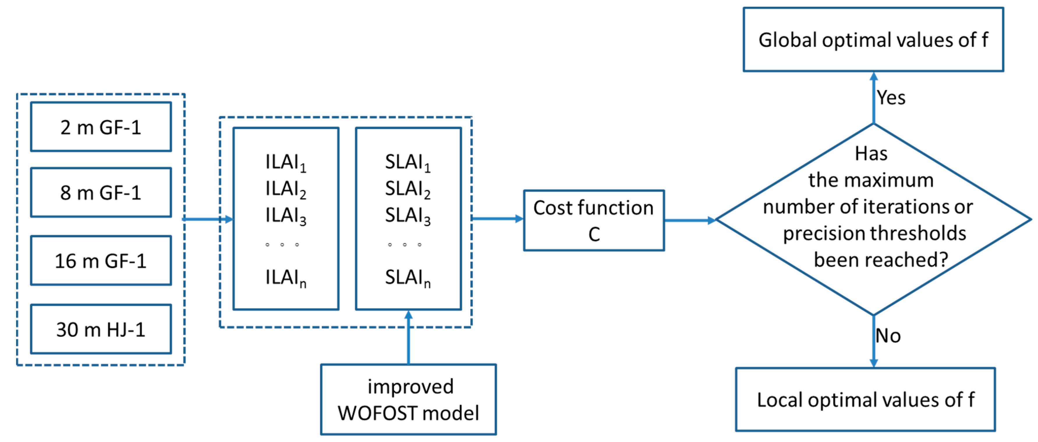
3.1. Computing LAI from GF-1 and HJ-1 Data
3.2. Extraction of WRT and WSO
3.3. Determination of the Heavy Metal Stress Condition Indicators
4. Results
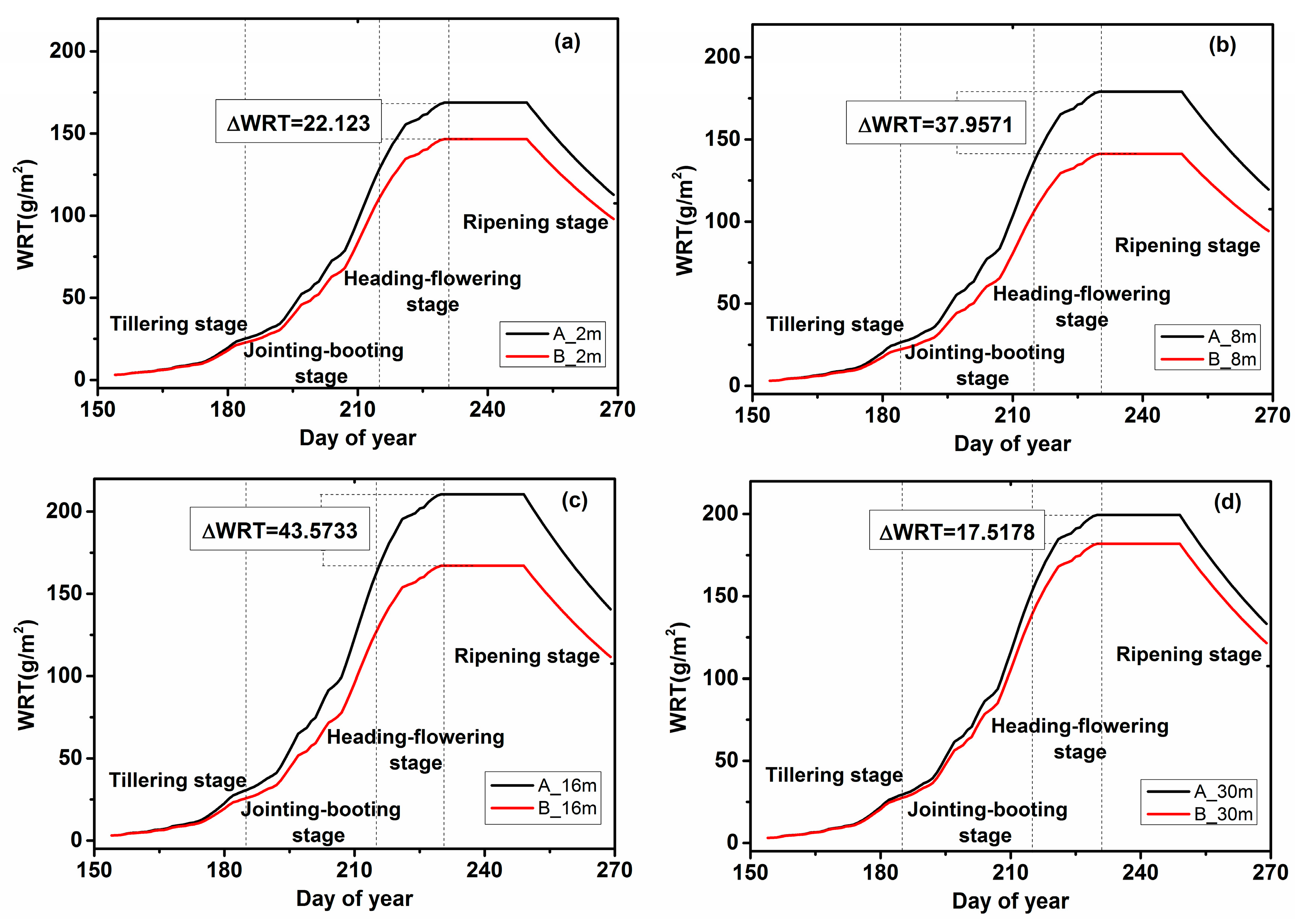
4.1. WRT Analysis
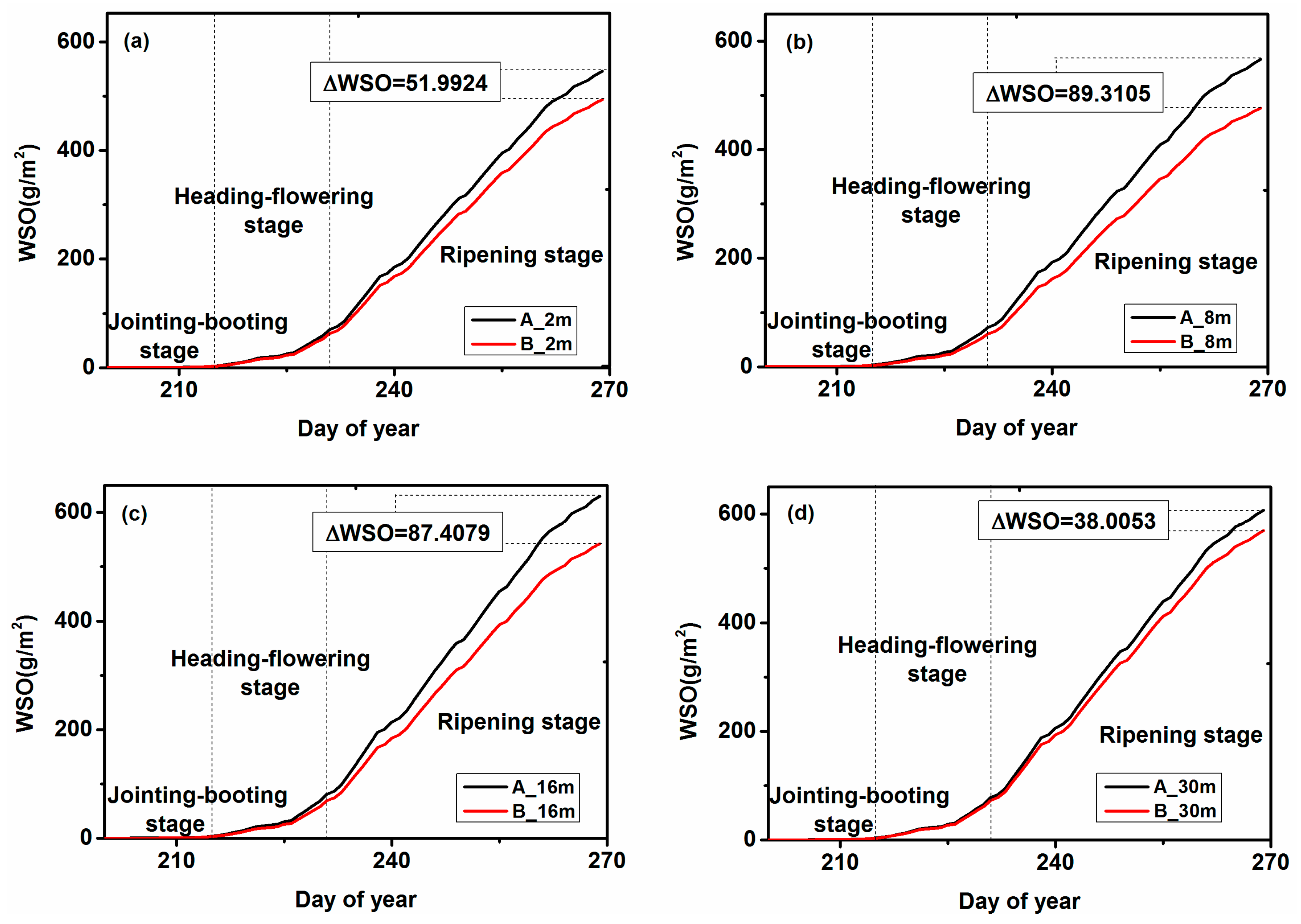
4.2. WSO Analysis
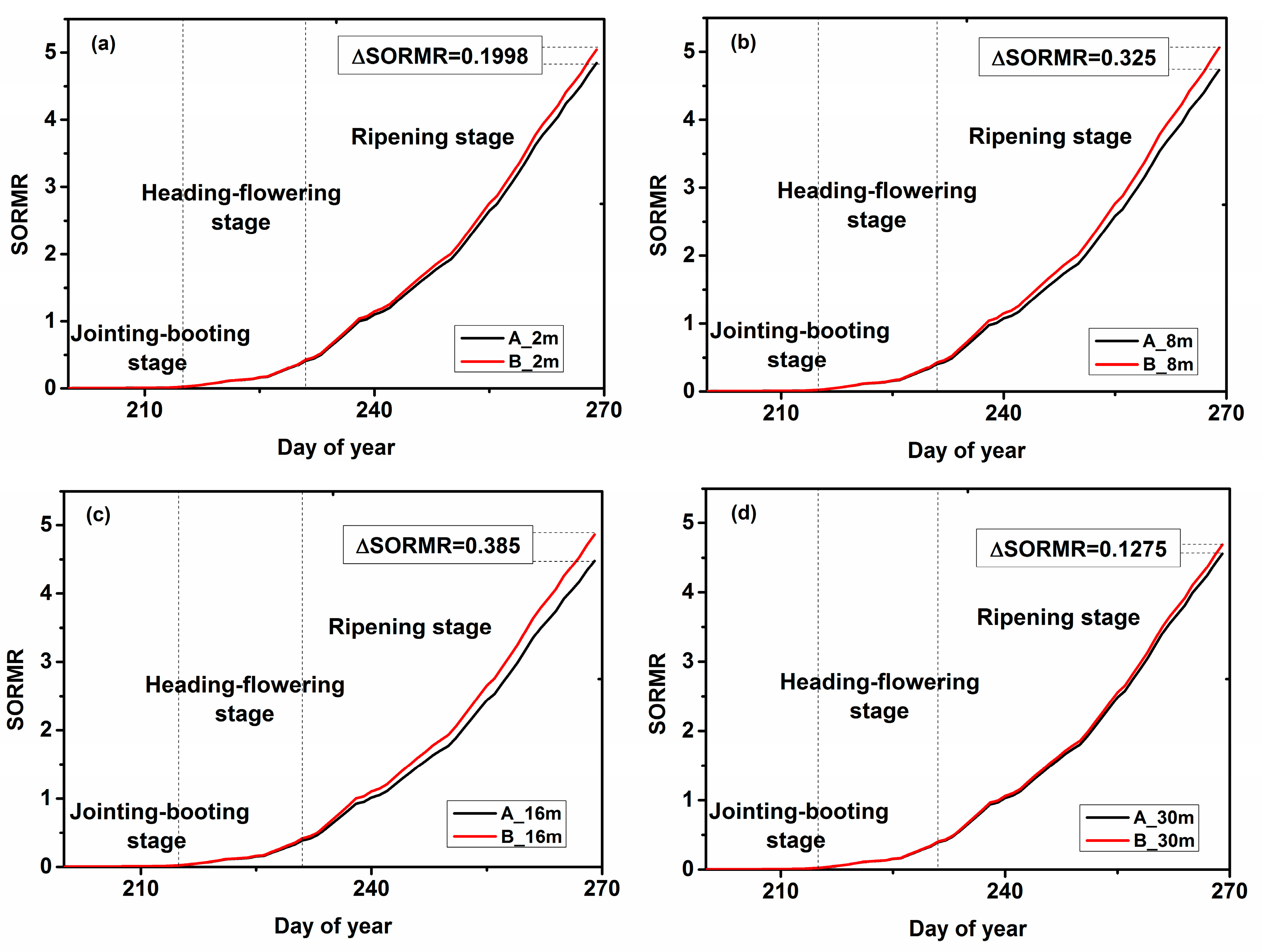
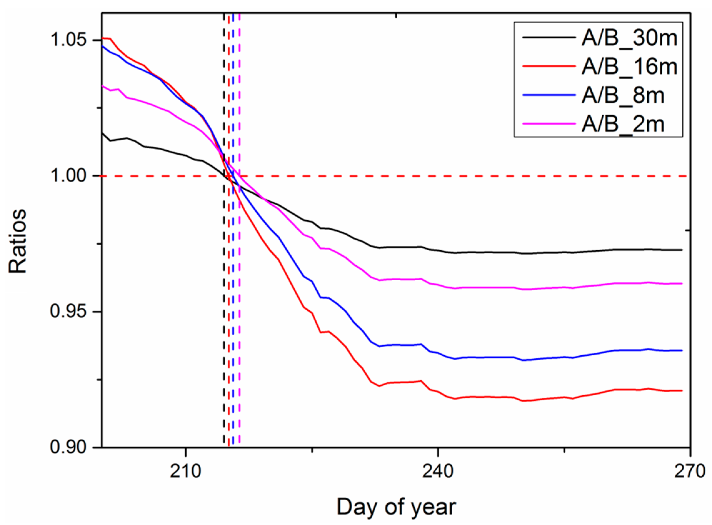
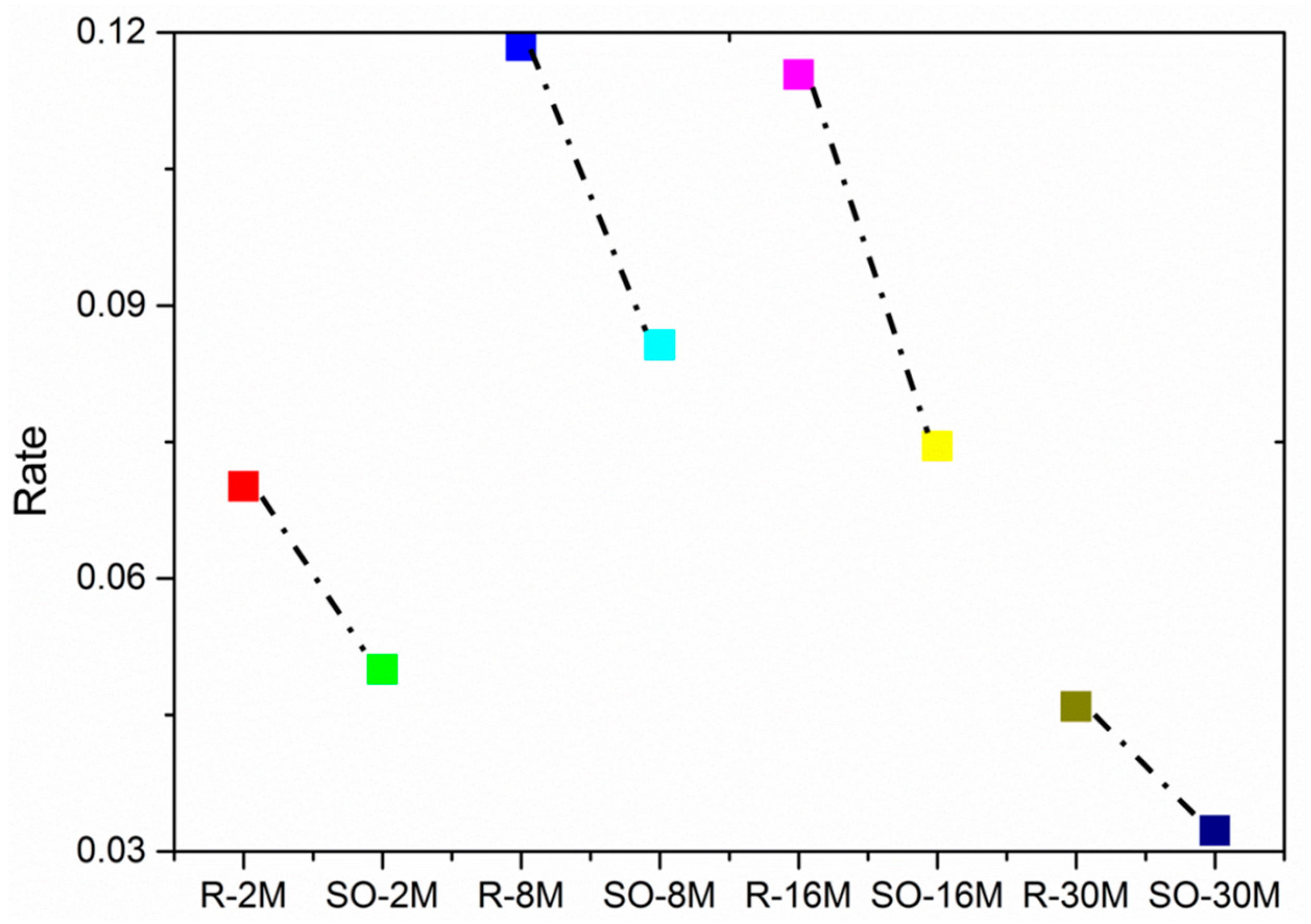
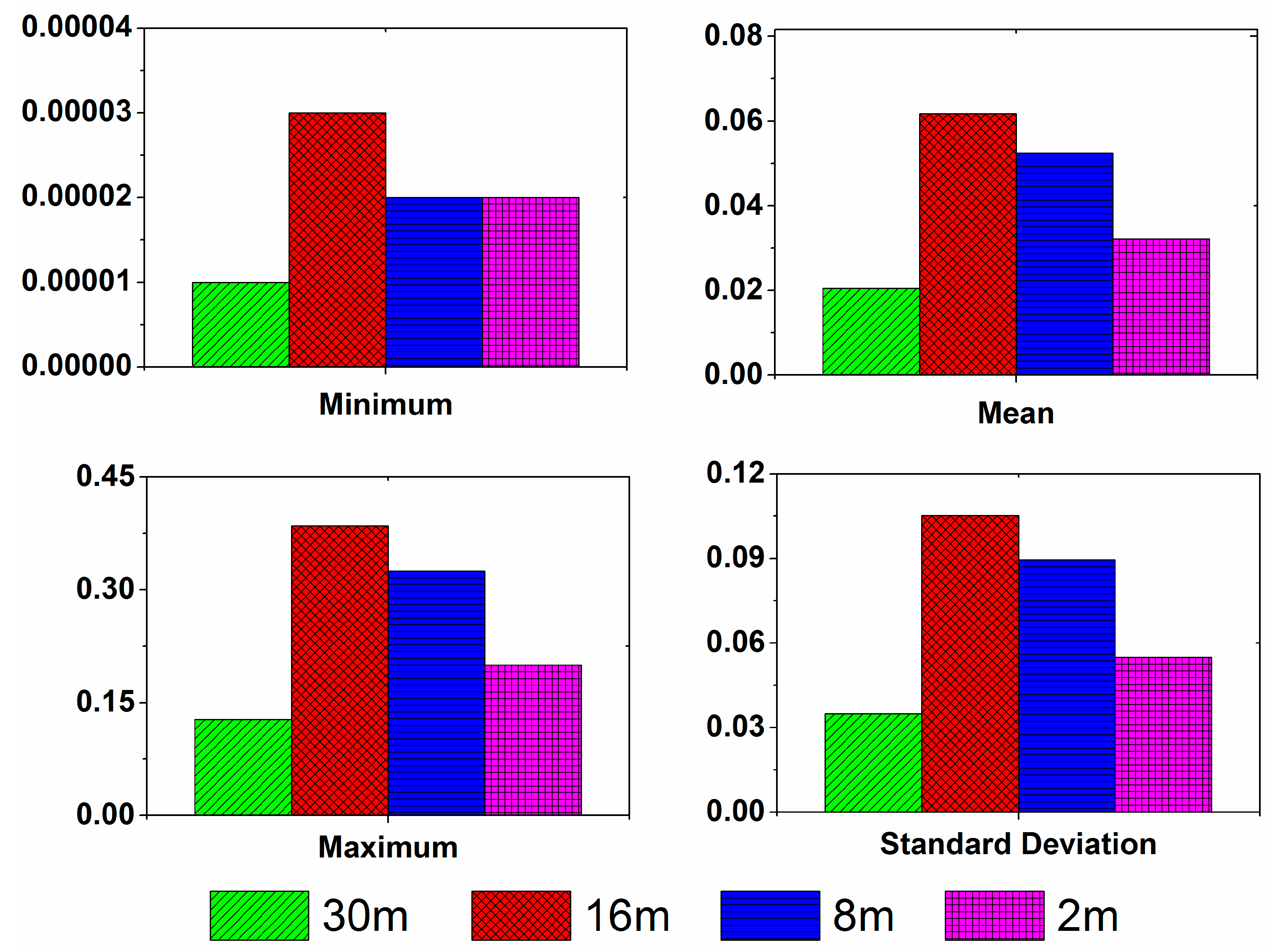
4.3. SORMR Analysis
5. Discussion
6. Conclusions
Acknowledgments
Author Contributions
Conflicts of Interest
References
- Fu, J.; Zhou, Q.; Liu, J.; Liu, W.; Wang, T.; Zhang, Q.; Jiang, G. High levels of heavy metals in rice (Oryza sativa L.) from a typical E-waste recycling area in southeast China and its potential risk to human health. Chemosphere 2008, 71, 1269–1275. [Google Scholar] [CrossRef] [PubMed]
- Zhang, J.-H.; Hang, M. Eco-toxicity and metal contamination of paddy soil in an e-wastes recycling area. J. Hazard. Mater. 2009, 165, 744–750. [Google Scholar]
- Chen, H. Changes of Seedlings Growth and Antioxidant Enzyme Activities of Different Cd-tolerant Rice Cultivars under Cadmium Stress. Acta Agric. Univ. Jiangxiensis 2012, 34, 1099–1104. [Google Scholar]
- He, J.Y.; Ren, Y.; Wang, Y. Root morphological and physiological responses of rice seedlings with different tolerance to cadmium stress. Acta Ecol. Sin. 2011, 31, 522–528. [Google Scholar]
- Choe, E.; Meer, F.V.D.; Ruitenbeek, F.V.; Werff, H.V.D.; Smeth, B.D.; Kim, K.W. Mapping of heavy metal pollution in stream sediments using combined geochemistry, field spectroscopy, and hyperspectral remote sensing: A case study of the Rodalquilar mining area, SE Spain. Remote Sens. Environ. 2008, 112, 3222–3233. [Google Scholar] [CrossRef]
- Kemper, T.; Sommer, S. Estimate of heavy metal contamination in soils after a mining accident using reflectance spectroscopy. Environ. Sci. Technol. 2002, 36, 2742–2747. [Google Scholar] [CrossRef] [PubMed]
- Liu, Y.; Wei, L.I.; Guofeng, W.U.; Xinguo, X.U. Feasibility of estimating heavy metal concentrations in Phragmites australis using laboratory-based hyperspectral data—A case study along Le’an River, China. Int. J. Appl. Earth Obs. Geoinf. 2010, 12, S166–S170. [Google Scholar] [CrossRef]
- Maruthi, S.B.B.; Vincent, R.K.; Roberts, S.J.; Czajkowski, K. Remote sensing of soybean stress as an indicator of chemical concentration of biosolid amended surface soils. Int. J. Appl. Earth Obs. Geoinf. 2011, 13, 676–681. [Google Scholar]
- Rosso, P.H.; Pushnik, J.C.; Lay, M.; Ustin, S.L. Reflectance properties and physiological responses of Salicornia virginica to heavy metal and petroleum contamination. Environ. Pollut. 2005, 137, 241–252. [Google Scholar] [CrossRef] [PubMed]
- Chi, G.; Huang, B.; Chen, X.; Shi, Y.; Zheng, T. Effects of Cadmium on Visible and Near-Infrared Reflectance Spectra of Rice (Oryza sativa L.). Fresenius Environ. Bull. 2011, 20, 391–397. [Google Scholar]
- Ren, H.Y.; Zhuang, D.; Pan, J.; Qiu, D. Canopy hyperspectral characteristics of paddy plants contaminated by lead. Geo-Inf. Sci. 2008, 10, 314–319. [Google Scholar]
- Ren, H.; Zhuang, D.F.; Pan, J.J.; Shi, X.Z.; Wang, H.J. Hyper-spectral remote sensing to monitor vegetation stress. J. Soils Sediments 2008, 8, 323. [Google Scholar] [CrossRef]
- McGwire, K.; Friedl, M.; Estes, J.E. Spatial structure, sampling design and scale in remotely-sensed imagery of a California savanna woodland. Remote Sens. 1993, 14, 2137–2164. [Google Scholar] [CrossRef]
- Peng, H.; Gong, J.Y. A review on choice of optimal scale in remote sensing. Remote Sens. Inf. 2008, 1, 96–99. [Google Scholar]
- Marceau, D.J.; Howarth, P.J.; Gratton, D.J. Remote sensing and the measurement of geographical entities in a forested environment. 2. The optimal spatial resolution. Remote Sens. Environ. 1994, 49, 105–117. [Google Scholar] [CrossRef]
- Woodcock, E.C.; Strahler, A.H. The factor of scale in remote sensing. Remote Sens. Environ. 1987, 21, 311–332. [Google Scholar] [CrossRef]
- Goodchild, M.F.; Quattrochi, D.A. Scale, Multiscaling, Remote Sensing, and GIS; CRC Press: Boca Raton, FL, USA, 1997; p. 406. [Google Scholar]
- Ming, D.P.; Wang, Q.; Yang, J.Y. Spatial scale of remote sensing image and selection of optimal spatial resolution. J. Remote Sens. 2008, 12, 529–537. [Google Scholar]
- Jurek, K.; Pickett, S.T.A. Ecological Heterogeneity; Springer: New York, NY, USA, 1991. [Google Scholar]
- Song, X.; Wang, R.; Yang, G.; Wang, J. Winter wheat growth spatial variability character analysis based on remote sensing image with high resolution. Trans. Chin. Soc. Agric. Eng. 2014, 30, 192–199. [Google Scholar]
- Wen, Z.F.; Zhang, S.; Bai, J.; Ding, C.; Zhang, C. Agricultural landscape spatial heterogeneity analysis and optimal scale selection: An example applied to Sanjiang plain. Acta Geogr. Sin. 2012, 67, 346–356. [Google Scholar]
- Garrigues, S.; Allard, D.; Baret, F.; Weiss, M. Quantifying spatial heterogeneity at the landscape scale using variogram models. Remote Sens. Environ. 2006, 103, 81–96. [Google Scholar] [CrossRef]
- Atkinson, P.M.; Curran, P.J. Curran. Choosing an appropriate spatial resolution for remote sensing investigations. Photogramm. Eng. Remote Sens. 1997, 63, 1345–1351. [Google Scholar]
- Lam, N.S.N.; Quattrochi, D.A. On the Issues of Scale, Resolution, and Fractal Analysis in the Mapping Sciences. Prof. Geogr. 1992, 44, 88–98. [Google Scholar] [CrossRef]
- Wang, L.; Yang, R.; Tian, Q.; Yang, Y.; Zhou, Y.; Sun, Y.; Mi, X. Comparative analysis of GF-1 WFV, ZY-3 MUX, and HJ-1 CCD sensor data for grassland monitoring applications. Remote Sens. 2015, 7, 2089–2108. [Google Scholar] [CrossRef]
- Wu, M.; Huang, W.; Niu, Z.; Wang, C. Combining HJ CCD, GF-1 WFV and MODIS data to generate daily high spatial resolution synthetic data for environmental process monitoring. Int. J. Environ. Res. Public Health 2015, 12, 9920–9937. [Google Scholar] [CrossRef] [PubMed]
- Li, H.; Chen, Z.X.; Jiang, Z.W.; Wu, W.-B.; Ren, J.Q.; Liu, B.; Tuya, H. Comparative analysis of GF-1, HJ-1, and Landsat-8 data for estimating the leaf area index of winter wheat. J. Integr. Agric. 2017, 16, 266–285. [Google Scholar] [CrossRef]
- Gallo, K.P.; Daughtry, C.S.T. Differences in vegetation indices for simulated Landsat-5 MSS and TM, NOAA-9 AVHRR, and SPOT-1 sensor systems. Remote Sens. Environ. 1987, 23, 439–452. [Google Scholar] [CrossRef]
- Aplin, P. Spatial variation in land cover and choice of spatial resolution for remote sensing. Int. J. Remote Sens. 2004, 25, 3687–3702. [Google Scholar]
- Chen, J.; Chen, T.; Mei, X.; Shao, Q.; Deng, M. Hilly farmland extraction from high resolution remote sensing imagery based on optimal scale selection. Trans. Chin. Soc. Agric. Eng. 2014, 30, 99–107. [Google Scholar]
- Yanchen, B.; Wang, J.; Li, X. Exploring the scale effect in land cover mapping from remotely sensed data: The statistical separability-based method. In Proceedings of the Geoscience and Remote Sensing Symposium, Seoul, Korea, 29 July 2005; pp. 3884–3887. [Google Scholar]
- Zhao, J.; Li, J.; Liu, Q.; Fan, W.; Zhong, B.; Wu, S.; Yang, L.; Zeng, Y.; Xu, B.; Yin, G. Leaf Area Index Retrieval Combining HJ1/CCD and Landsat8/OLI Data in the Heihe River Basin, China. Remote Sens. 2015, 7, 6862–6885. [Google Scholar] [CrossRef]
- Song, Q.; Hu, Q.; Zhou, Q.; Hovis, C.; Xiang, M.; Tang, H.; Wu, W. In-Season Crop Mapping with GF-1/WFV Data by Combining Object-Based Image Analysis and Random Forest. Remote Sens. 2017, 9, 1184. [Google Scholar] [CrossRef]
- Zhou, Y.; Lin, C.; Wang, S.; Liu, W.; Tian, Y. Estimation of Building Density with the Integrated Use of GF-1 PMS and Radarsat-2 Data. Remote Sens. 2016, 8, 969. [Google Scholar] [CrossRef]
- Soudani, K.; François, C.; Maire, G.L.; Dantec, V.L.; Dufrêne, E. Comparative analysis of IKONOS, SPOT, and ETM+ data for leaf area index estimation in temperate coniferous and deciduous forest stands. Remote Sens. Environ. 2006, 102, 161–175. [Google Scholar] [CrossRef] [Green Version]
- Wang, L.; Dong, T.; Zhang, G.; Niu, Z. LAI retrieval using PROSAIL model and optimal angle combination of multi-angular data in wheat. IEEE J. Sel. Top. Appl. Earth Obs. Remote Sens. 2013, 6, 1730–1736. [Google Scholar] [CrossRef]
- Posner, A.; Georgakakos, K.; Shamir, E. MODIS inundation estimate assimilation into soil moisture accounting hydrologic model: A case study in Southeast Asia. Remote Sens. 2014, 6, 10835–10859. [Google Scholar] [CrossRef]
- Dorigo, W.A.; Zurita-Milla, R.; Wit, A.J.W.D.; Brazile, J.; Singh, R.; Schaepman, M.E. A review on reflective remote sensing and data assimilation techniques for enhanced agroecosystem modeling. Int. J. Appl. Earth Obs. Geoinf. 2007, 9, 165–193. [Google Scholar] [CrossRef]
- Machwitz, M.; Giustarini, L.; Bossung, C.; Frantz, D.; Schlerf, M.; Lilienthal, H.; Wandera, L.; Matgen, P.; Hoffmann, L.; Udelhoven, T. Enhanced biomass prediction by assimilating satellite data into a crop growth model. Environ. Model. Softw. 2014, 62, 437–453. [Google Scholar] [CrossRef]
- Chen, Y.; Chi, W.C.; Huang, T.L.; Lin, C.Y.; Nguyeh, T.T.Q.; Hsiung, Y.C.; Chia, L.C.; Huang, H.J. Mercury-induced biochemical and proteomic changes in rice roots. Plant Physiol. Biochem. 2012, 55, 23–32. [Google Scholar] [CrossRef] [PubMed]
- Kang, L.-J.; Zhao, M.; Zhuang, G. Accumulation of cu as single and complex pollutants in rice. J. Agro-Environ. Sci. 2003, 22, 503–504. [Google Scholar]
- Xu, J.; Yang, L.; Wang, Y.; Wang, Z. Advances in the study uptake and accumulation of heavy metal in rice ({\sl Oryza sativa}) and its mechanisms. Chin. Bull. Bot. 2004, 22, 614–622. [Google Scholar]
- Huang, Z.; Liu, X.; Jin, M.; Ding, C.; Jiang, J.; Wu, L. Deriving the characteristic scale for effectively monitoring heavy metal stress in rice by assimilation of GF-1 data with the wofost model. Sensors 2016, 16, 340. [Google Scholar] [CrossRef] [PubMed]
- Liu, M.; Liu, X.; Liu, M.; Liu, F.; Jin, M.; Wu, L. Root mass ratio: Index derived by assimilation of synthetic aperture radar and the improved World Food Study model for heavy metal stress monitoring in rice. J. Appl. Remote Sens. 2016, 10, 026038. [Google Scholar] [CrossRef]
- Wang, H. Effects of single and combined pollution of Pb, Cd and Cu on growth, metal uptake and translocation in rice. In Proceedings of the International Conference on Mechatronics, Materials, Biotechnology and Environment, Yinchuan, China, 13–14 August 2016. [Google Scholar]
- Cao, F.B.; Ahmed, I.M.; Zheng, W.; Zhang, G.; Wu, F. Genotypic and environmental variation of heavy metal concentrations in rice grains. J. Food Agric. Environ. 2013, 11, 718–724. [Google Scholar]
- Lou, Y.; Peng, Z.; Wang, D.; Amombo, E.; Xin, S.; Hui, W.; Zhuge, Y. Germination, Physiological Responses and Gene Expression of Tall Fescue (Festuca arundinacea Schreb.) Growing under Pb and Cd. PLoS ONE 2017, 12, e0169495. [Google Scholar] [CrossRef] [PubMed]
- Wang, F.-M.; Huang, J.-F.; Tang, Y.-L.; Wang, X.-Z. New vegetation index and its application in estimating leaf area index of rice. Rice Sci. 2007, 14, 195–203. [Google Scholar] [CrossRef]
- Yoder, B.J.; Waring, R.H. The normalized difference vegetation index of small Douglas-fir canopies with varying chlorophyll concentrations. Remote Sens. Environ. 1994, 49, 81–91. [Google Scholar] [CrossRef]
- Zhang, J.C.; Gu, X.H.; Wang, J.H.; Huang, W.J.; He, X.; Wang, H.F. Analysis of consistency between HJ-CCD images and TM images in monitoring rice LAI. Trans. Chin. Soc. Agric. Eng. 2010, 26, 186–193. [Google Scholar]
- Jin, M.; Liu, X.; Wu, L.; Liu, M. Distinguishing heavy-metal stress levels in rice using synthetic spectral index responses to physiological function variations. IEEE J. Sel. Top. Appl. Earth Obs. Remote Sens. 2017, 10, 75–86. [Google Scholar] [CrossRef]
- Boogaard, H.L. User’s Guide for the WOFOST 7.1 Crop Growth Simulation Model and WOFOST Control Center 1.5 Technical Document 52 DLO Vinand Staring Centre; Winand Staring Centre for Integrated Land, Soil and Water Research: São Paulo, Brazil, 1998. [Google Scholar]
- Tchomté, S.K.; Gourgand, M. Particle swarm optimization: A study of particle displacement for solving continuous and combinatorial optimization problems. Int. J. Prod. Econ. 2009, 121, 57–67. [Google Scholar] [CrossRef]
- Wu, L.; Liu, X.; Wang, P.; Zhou, B.; Liu, M.; Li, X. The assimilation of spectral sensing and the WOFOST model for the dynamic simulation of cadmium accumulation in rice tissues. Int. J. Appl. Earth Obs. Geoinf. 2013, 25, 66–75. [Google Scholar] [CrossRef]
- Liu, F.; Liu, X.; Ding, C.; Wu, L. The dynamic simulation of rice growth parameters under cadmium stress with the assimilation of multi-period spectral indices and crop model. Field Crop. Res. 2015, 183, 225–234. [Google Scholar] [CrossRef]
- Khan, S.; Cao, Q.; Zheng, Y.M.; Huang, Y.Z.; Zhu, Y.G. Health risks of heavy metals in contaminated soils and food crops irrigated with wastewater in Beijing, China. Environ. Pollut. 2008, 152, 686–692. [Google Scholar] [CrossRef] [PubMed]
- Marceau, D.J.; Hay, G.J. Remote sensing contributions to the scale issue. Can. J. Remote Sens. 1999, 25, 357–366. [Google Scholar] [CrossRef]


| Study Area | Type | Cd | Hg | Pb | As | Pollution Level |
|---|---|---|---|---|---|---|
| A | Soil | 0.84 | 0.25 | 78.32 | 10.22 | Low |
| Rice Tissue | 0.82 | 0.04 | 10.60 | 5.39 | ||
| Pollution index | 0.59 | 1.25 | 0.95 | 0.53 | ||
| B | Soil | 3.28 | 0.51 | 120.75 | 18.15 | High |
| Rice Tissue | 5.90 | 0.06 | 36.73 | 7.04 | ||
| Pollution index | 2.29 | 2.55 | 1.46 | 0.95 | ||
| Background value | 1.43 | 0.2 | 82.78 | 19.11 |
| Sensor | Spatial Resolution (m) | Revisitation Period (day) | Breadth (km) | Band 1 (nm) | Band 2 (nm) | Band 3 (nm) | Band 4 (nm) |
|---|---|---|---|---|---|---|---|
| GF-1 | 2 | 4 | 60 | 0.45~0.90 | |||
| 8 | 4 | 60 | 0.45~0.52 | 0.52~0.59 | 0.63~0.69 | 0.77~0.89 | |
| 16 | 2 | 800 | 0.45~0.52 | 0.52~0.59 | 0.63~0.69 | 0.77~0.89 | |
| HJ-1 | 30 | 4 | 360 (1CCD) 700 (2CCD) | 0.43~0.52 | 0.52~0.60 | 0.63~0.69 | 0.76~0.90 |
| Statistical Analysis | A_30m | B_30m | A_16m | B_16m | A_8m | B_8m | A_2m | B_2m |
|---|---|---|---|---|---|---|---|---|
| Mean | 0.819 | 0.781 | 0.8447 | 0.7484 | 0.775 | 0.691 | 0.7518 | 0.704 |
| Minimum | 0.775 | 0.6 | 0.705 | 0.6 | 0.664 | 0.6 | 0.6 | 0.6 |
| Maximum | 0.9171 | 0.95 | 0.95 | 0.8161 | 0.9462 | 0.783 | 0.8851 | 0.775 |
| Statistical Analysis | A_30m | B_30m | A_16m | B_16m | A_8m | B_8m | A_2m | B_2m |
|---|---|---|---|---|---|---|---|---|
| Minimum | 0.00030 | 0.00029 | 0.00031 | 0.00028 | 0.00029 | 0.00027 | 0.00029 | 0.00027 |
| Mean | 0.73376 | 0.75426 | 1.72085 | 0.7826 | 0.76162 | 0.81404 | 0.77959 | 0.81175 |
| Maximum | 4.55944 | 4.6869 | 4.47896 | 4.86346 | 4.73293 | 5.05791 | 4.84456 | 5.04432 |
| Standard Deviation | 1.23371 | 1.26862 | 1.21164 | 1.31682 | 1.28115 | 1.37043 | 1.31164 | 1.3665 |
© 2018 by the authors. Licensee MDPI, Basel, Switzerland. This article is an open access article distributed under the terms and conditions of the Creative Commons Attribution (CC BY) license (http://creativecommons.org/licenses/by/4.0/).
Share and Cite
Wang, D.; Liu, X. Comparative Analysis of GF-1 and HJ-1 Data to Derive the Optimal Scale for Monitoring Heavy Metal Stress in Rice. Int. J. Environ. Res. Public Health 2018, 15, 461. https://doi.org/10.3390/ijerph15030461
Wang D, Liu X. Comparative Analysis of GF-1 and HJ-1 Data to Derive the Optimal Scale for Monitoring Heavy Metal Stress in Rice. International Journal of Environmental Research and Public Health. 2018; 15(3):461. https://doi.org/10.3390/ijerph15030461
Chicago/Turabian StyleWang, Dongmin, and Xiangnan Liu. 2018. "Comparative Analysis of GF-1 and HJ-1 Data to Derive the Optimal Scale for Monitoring Heavy Metal Stress in Rice" International Journal of Environmental Research and Public Health 15, no. 3: 461. https://doi.org/10.3390/ijerph15030461