Using a Counting Process Method to Impute Censored Follow-Up Time Data


Centre for Clinical Epidemiology and Biostatistics (CCEB), School of Medicine and Public Health, The University of Newcastle (UoN), Callaghan, NSW 2308, Australia
*
Author to whom correspondence should be addressed.
Int. J. Environ. Res. Public Health 2018, 15(4), 690; https://doi.org/10.3390/ijerph15040690
Submission received: 17 March 2018
/
Revised: 1 April 2018
/
Accepted: 3 April 2018
/
Published: 5 April 2018
(This article belongs to the Special Issue Selected Paper from the 14th International Symposium on Recent Advances in Environmental Health Research)
Abstract
:Censoring occurs when complete follow-up time information is unavailable for patients enrolled in a clinical study. The process is considered to be informative (non-ignorable) if the likelihood function for the model cannot be partitioned into a set of response parameters that are independent of the censoring parameters. In such cases, estimated survival time probabilities may be biased, prompting the need for special statistical methods to remedy the situation. The problem is especially salient when censoring occurs early in a study. In this paper, we describe a method to impute censored follow-up times using a counting process method.
1. Introduction
Ideally, censoring in a survival analysis should be non-informative and not related to any aspect of the study that could bias results [1,2,3,4,5,6,7]. For example, toxic side effects of an investigational drug may prompt the most ill patients to withdraw early from the study. Other patients may opt to leave before the intended end of a trial if the treatment is effective and they feel well. Even when censoring is non-informative (e.g., relocation to another city because of plant closure), by chance alone, it may still have a serious effect on estimated survival probabilities, especially if the dropouts occur early in the study.
In this paper, we present an example of early censoring to illustrate how the resulting survival probabilities may be biased. We then describe a method to impute censored follow-up times by rearranging the data as a counting process and generating jump-point plots.
2. Materials and Methods
Imputing Censored Follow-Up Times
Let denote the follow-up time for the ordered observation, given a total of observations and integer valued time points. Accordingly,
and
Then, for all values of and over their respective ranges (i.e., ), the counting process “indicator” variable assumes the value 0 if and corresponds to a censored follow-up time (i.e., the outcome event, such as death, has yet to occurred by time ). Otherwise, when the observation denotes an event, assumes the value 0 if and the value 1 if [8].
Next, we fit a multiple logistic regression model with covariates to the above counting process data, i.e.,
where the first covariate denotes time and the remaining covariates represent outcome related risk factors. Model adequacy may be assessed by examining diagnostic plots, in lieu of standard goodness-of-fit tests, which would assume that the underlying counting process data are independently distributed [9,10,11,12]. In some cases, including higher-order or trigonometric terms into the logistic regression equation may improve model fit.
A jump-point plot for a particular covariate pattern corresponding to a censored follow-up time may be obtained by plotting the model predicted values against the time variable . Let denote the value of that maps to (i.e., maximum likelihood estimate of the mean jump-point observation). The imputed censored follow-up time is given as
where is the natural upper limit for a patient’s follow-up time. For example, in the case of cancer therapy, the maximum life expectancy of a patient rarely exceeds 101 years of age. For a patient aged 89 at diagnosis, we see that is computed as (101 minus 89) The original censored follow-up times are then replaced with . However, it is important to note that these follow-up times are still treated as censored values rather than events when computing survival probability estimates.
Assuming Martingale independence and considering the event times to be binomially distributed (i.e., the probability of an event occurring in a particular risk set is equal to its expectation divided by the risk set size (accounting for censored and event times), with corresponding variance equal to ), it follows that the resulting data be may analyzed using standard methods for handling censored time-to-event observations (e.g., Kaplan-Meier and Cox proportional-hazards models) [13,14]. Here, the sampling variability for estimating the imputed censored follow-up times is absorbed into the sampling variability for each binomially distributed event time, given that the estimates are asymptotically consistent and adhere to certain regularity conditions.
3. Results
3.1. Kaplan-Meier (Product-Limit) Example
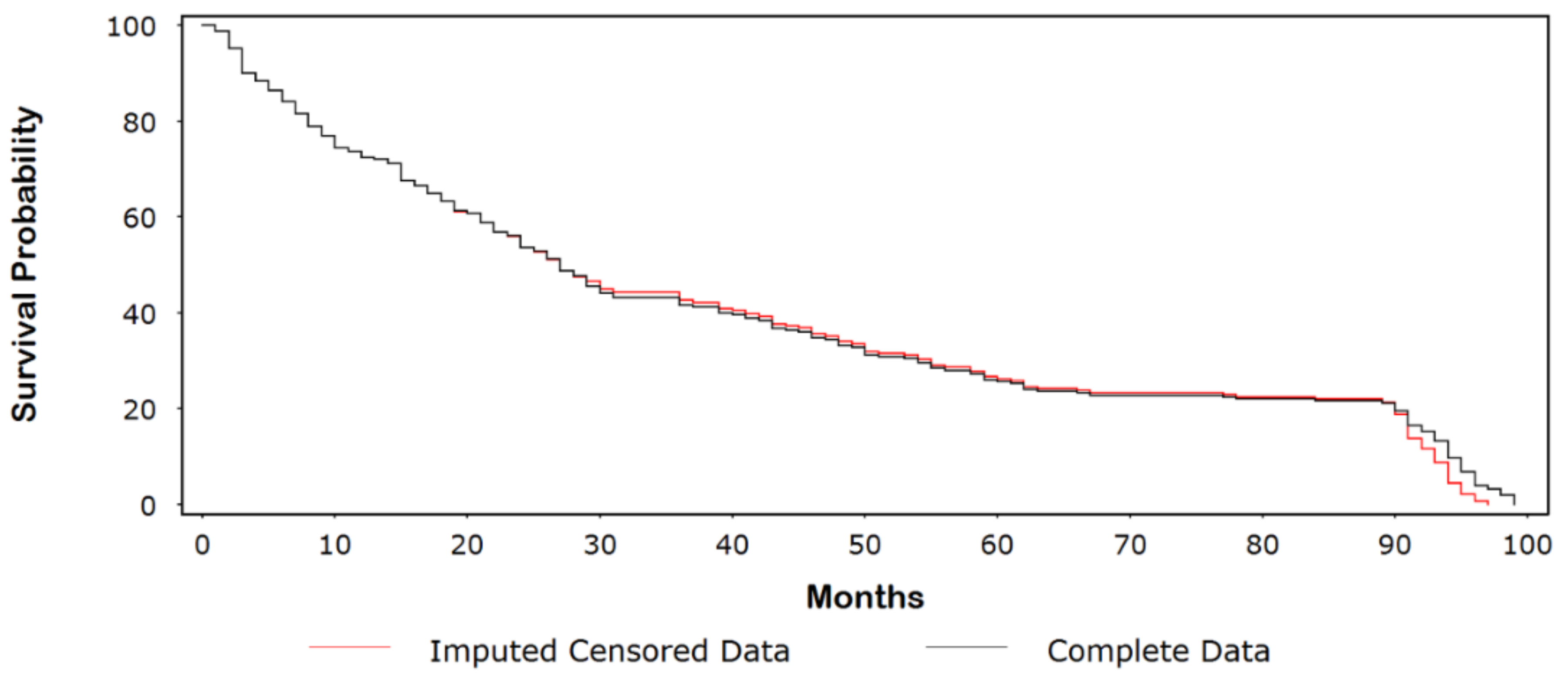
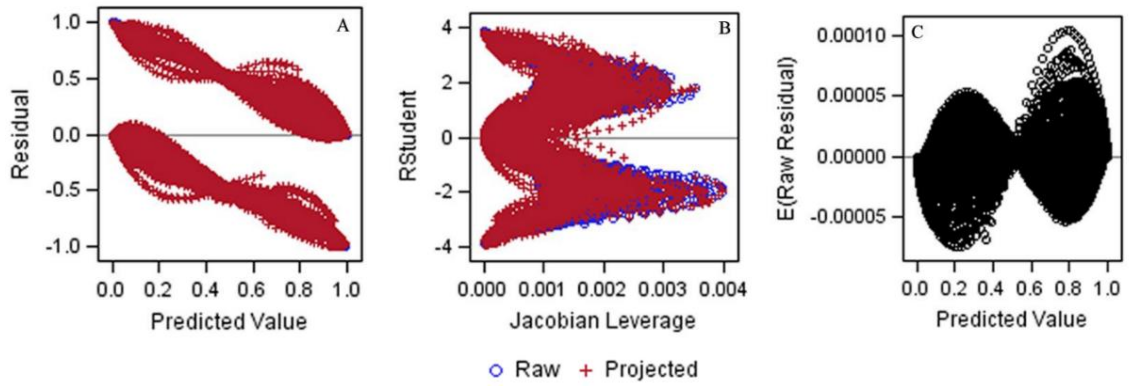
Consider the data in Table A1, which provides the event and censored follow-up times for 250 cancer patients undergoing treatment and their simulated complete values (for illustrative purposes). Approximately 10% of the follow-up times were censored, with the majority of these values occurring early in the study. Figure 1 shows a Kaplan-Meir (KM) plot comparing the original censored data with the dataset of complete follow-up times. The probability of surviving 5 years (60 months) was ~26% for the original censored data compared with ~18% for the complete dataset. In Figure 2, we compare the complete dataset with the imputed censored dataset. At 5 years, rounding to the nearest whole number, we see that the survival times are identical (i.e., 26%). Indeed, the curves are similar until ~90 months, at which point the survival times for the imputed censored time curve are divergently lower than those for the complete dataset. In Figure 3A–C, we observed a few outlying values that indicate a nominal departure from the underlying model goodness-of-fit.
3.2. Generating the Jump-Point Plot
The jump-point plot corresponding to the covariate pattern
is shown in Figure 4. Here, the variables correspond to age (years), grade (I-IV), lymph node invasion (1 = yes, 0 = no), positive margins (1 = yes, 0 = no), no hormone therapy (1 = yes, 0 = no), and no radiation therapy (1 = yes, 0 = no), respectively. We see that the imputed censored follow-up time of 29.33 months closely matches the actual event time of 29 months. This observation was originally censored at 1 month.
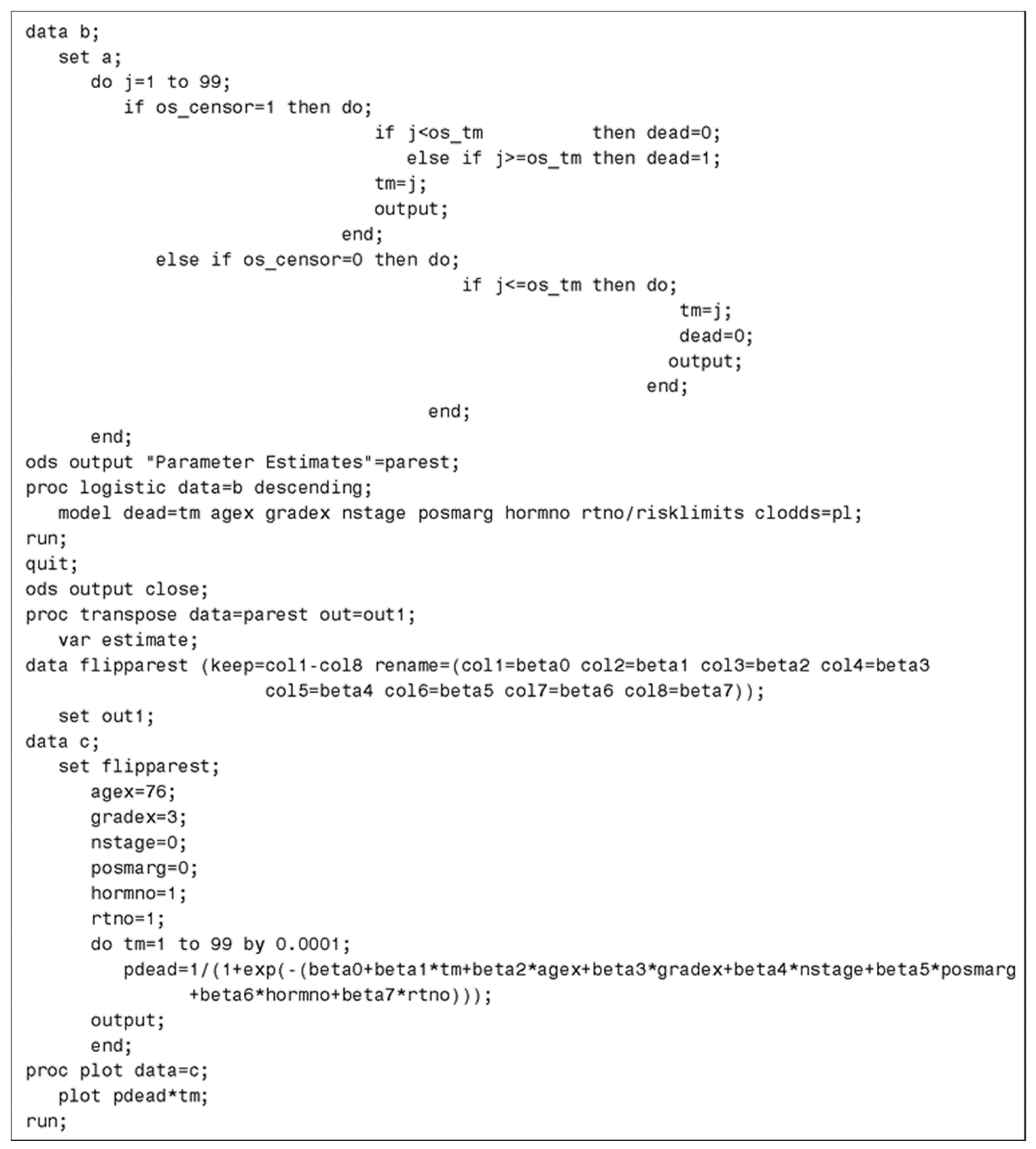
3.3. SAS Code
The SAS code used to generate the jump-point plot is shown in Figure 5. In this code, it is assumed that the data contained in Appendix A has been previously read into the dataset “a”. The counting process variables are created in dataset “b” and then modeled using the “PROC LOGISTIC” procedure. The predicted probabilities generated by this procedure are plotted against time (ranging from 1 to 99 months) to obtain the jump-point plot. Analyses were performed using SAS Version 9.4. (SAS Institute, Cary, NC, USA).
4. Discussion
In this manuscript, we have introduced a simple method to partially correct for non-ignorable early censoring. By rearranging the data as a counting process, we are able to account for the follow-up times of all patients, regardless of their censoring status. For example, if a patient is censored at 50 months, the counting process creates 50 observations corresponding to each month and accordingly assigns the value of 0 to an indicator variable. On the other hand, if the patient had an event at 50 months, the counting process would create 49 observations with the indicator variable set to 0 and similarly create new observations for each month thereafter until the last month of the study, but instead assigning the value of 1 to the indicator variable.
These counting responses are then analyzed with logistic regression. In addition to including outcome-related covariates, a variable denoting the time (e.g., month) associated with the indicator variable is added to the model. The predicted value generated by the model for a particular covariate pattern (associated with a censored observation) is then plotted against the time variable (spanning each month of the study) to obtain a jump-point plot. Dropping a line from the midpoint of this plot to the x-axis gives an imputed censored follow-up time. We then replace the original censored time with this value if it is the larger of the two values. Additionally, the imputed value is constrained by a natural upper bound to prevent impossible censored follow-up times (e.g., the value must be consistent with a patient’s maximum biologic lifespan).
An important aspect of this technique is identifying a well-fitting model for the counting process data so that it is able to accurately predict if the outcome is 0 or 1. Understanding the dynamics of the disease or process under study will aid in the selection of appropriate outcome-related covariates. However, formally testing for model goodness-of-fit is not practical given the highly correlated nature of the counting process data. In theory, while it may be possible to assess model goodness-of-fit for dependent data using a robust “Huber-White” approach, the regularity conditions for such estimates are quite stringent [15,16,17].
Instead, we recommend using diagnostic plots to rule out ill-fitting models [9,10,11]. As shown in our example, when the Jacobian leverages (defined as the instantaneous rate of change in the predictive value with respect to the outcome) were plotted against the studentized residuals, we observed outlying values towards the upper right hand side of this plot (Figure 3B). Correspondingly, we also noticed the presence of extreme points in the lower right-hand side of Figure 3A (which plots predicted values against their residuals) and the upper right portion of Figure 3C (which plots predictive values against their expected raw residuals). Nonetheless, the plots provided in Figure 3A–C were relatively symmetrical with respect to the positive and negative residuals, suggesting that the logistic regression model provided a reasonable fit to the counting process data [18].
The advantage of using a counting process approach is that the imputed censored follow-up times, when appropriately constructed, will better reflect the survival prospects of those who continued in the study. However, because the method is model based, it may not be suitable for small datasets or those lacking a set of reasonably predictive covariates. Additionally, it may not always be possible to identify a well-fitting model if there are abrupt changes in the hazard function of the underlying data. The method at hand should not be used if patients who enroll later in study survive longer (e.g., treatment improves over time) or if enrollment criteria change over the course of the study (e.g., worst patients are excluded midway through recruitment) [3].
5. Conclusions
Overall, the best means for handling informative censoring is to avoid the problem in the first place. Careful planning at the study design stage, routine patient monitoring, and implementing proactive strategies to minimize patient dropout are some important steps to ensure the fidelity of a survival time study.
Acknowledgments
Authors would like to thank the Centre for Clinical Epidemiology and Biostatistics, University of Newcastle, for support and technical assistance during the preparation of this manuscript.
Author Contributions
Jimmy T. Efird and Charulata Jindal conceived and designed the project, analyzed the data, and wrote the manuscript. Both authors approved the final version of the manuscript.
Conflicts of Interest
The authors declared no conflict of interest.
Appendix A

Table A1.
Example Cancer Dataset (N = 250). A = Observation number, B = Age, C = Grade, D = Lymph node invasion, E = Positive margin, F = No hormonal therapy, G = No radiation therapy, H = Actual follow-up time, I = Original censored time, J = Imputed censored time, K = Censoring variable.
Table A1.
Example Cancer Dataset (N = 250). A = Observation number, B = Age, C = Grade, D = Lymph node invasion, E = Positive margin, F = No hormonal therapy, G = No radiation therapy, H = Actual follow-up time, I = Original censored time, J = Imputed censored time, K = Censoring variable.
| A | B | C | D | E | F | G | H | I | J | K | A | B | C | D | E | F | G | H | I | J | K | A | B | C | D | E | F | G | H | I | J | K |
| 1 | 93 | 4 | 1 | 1 | 1 | 1 | 1 | 1 | -- | 1 | 36 | 96 | 4 | 1 | 0 | 1 | 1 | 6 | 6 | -- | 1 | 71 | 99 | 3 | 0 | 0 | 1 | 1 | 14 | 14 | -- | 1 |
| 2 | 90 | 3 | 1 | 1 | 1 | 1 | 1 | 1 | -- | 1 | 37 | 93 | 3 | 1 | 0 | 1 | 1 | 6 | 6 | -- | 1 | 72 | 83 | 2 | 1 | 1 | 1 | 1 | 14 | 14 | -- | 1 |
| 3 | 89 | 4 | 1 | 1 | 1 | 1 | 1 | 1 | -- | 1 | 38 | 94 | 3 | 1 | 0 | 0 | 1 | 6 | 6 | -- | 1 | 73 | 85 | 4 | 1 | 1 | 0 | 1 | 15 | 15 | -- | 1 |
| 4 | 89 | 4 | 1 | 0 | 1 | 1 | 2 | 2 | -- | 1 | 39 | 93 | 3 | 1 | 1 | 1 | 1 | 6 | 6 | -- | 1 | 74 | 83 | 3 | 1 | 1 | 0 | 1 | 15 | 15 | -- | 1 |
| 5 | 86 | 3 | 1 | 1 | 1 | 0 | 2 | 2 | -- | 1 | 40 | 97 | 3 | 1 | 1 | 1 | 1 | 6 | 6 | -- | 1 | 75 | 81 | 3 | 1 | 0 | 1 | 1 | 15 | 15 | -- | 1 |
| 6 | 86 | 3 | 1 | 0 | 1 | 1 | 2 | 2 | -- | 1 | 41 | 97 | 3 | 1 | 0 | 1 | 1 | 7 | 7 | -- | 1 | 76 | 98 | 1 | 1 | 0 | 0 | 1 | 15 | 15 | -- | 1 |
| 7 | 95 | 4 | 1 | 1 | 1 | 1 | 2 | 2 | -- | 1 | 42 | 97 | 2 | 1 | 0 | 1 | 1 | 7 | 7 | -- | 1 | 77 | 94 | 3 | 1 | 0 | 0 | 1 | 15 | 15 | -- | 1 |
| 8 | 90 | 3 | 1 | 1 | 1 | 1 | 2 | 2 | -- | 1 | 43 | 86 | 3 | 1 | 1 | 1 | 1 | 7 | 7 | -- | 1 | 78 | 93 | 4 | 1 | 0 | 0 | 0 | 15 | 15 | -- | 1 |
| 9 | 86 | 3 | 0 | 1 | 1 | 1 | 2 | 2 | -- | 1 | 44 | 85 | 3 | 1 | 0 | 1 | 1 | 7 | 7 | -- | 1 | 79 | 90 | 2 | 1 | 0 | 1 | 1 | 15 | 15 | -- | 1 |
| 10 | 84 | 4 | 1 | 0 | 0 | 1 | 2 | 2 | -- | 1 | 45 | 91 | 3 | 1 | 0 | 1 | 1 | 7 | 7 | -- | 1 | 80 | 88 | 3 | 1 | 0 | 1 | 1 | 15 | 15 | -- | 1 |
| 11 | 82 | 4 | 1 | 0 | 1 | 1 | 2 | 2 | -- | 1 | 46 | 94 | 3 | 1 | 1 | 1 | 1 | 7 | 7 | -- | 1 | 81 | 82 | 3 | 1 | 0 | 1 | 1 | 15 | 15 | -- | 1 |
| 12 | 91 | 2 | 1 | 1 | 1 | 1 | 2 | 2 | -- | 1 | 47 | 86 | 3 | 1 | 0 | 1 | 1 | 8 | 8 | -- | 1 | 82 | 85 | 4 | 1 | 1 | 0 | 0 | 16 | 16 | -- | 1 |
| 13 | 96 | 4 | 1 | 0 | 0 | 1 | 3 | 3 | -- | 1 | 48 | 86 | 4 | 1 | 0 | 1 | 1 | 8 | 8 | -- | 1 | 83 | 88 | 2 | 1 | 0 | 0 | 0 | 16 | 16 | -- | 1 |
| 14 | 95 | 3 | 1 | 0 | 1 | 1 | 3 | 3 | -- | 1 | 49 | 83 | 1 | 1 | 1 | 0 | 1 | 8 | 8 | -- | 1 | 84 | 82 | 3 | 1 | 0 | 1 | 0 | 16 | 16 | -- | 1 |
| 15 | 89 | 2 | 1 | 1 | 1 | 1 | 3 | 3 | -- | 1 | 50 | 96 | 3 | 1 | 1 | 1 | 1 | 8 | 8 | -- | 1 | 85 | 84 | 4 | 1 | 1 | 0 | 0 | 17 | 17 | -- | 1 |
| 16 | 88 | 4 | 1 | 0 | 1 | 0 | 3 | 3 | -- | 1 | 51 | 94 | 4 | 1 | 0 | 0 | 1 | 8 | 8 | -- | 1 | 86 | 90 | 2 | 1 | 1 | 0 | 1 | 17 | 17 | -- | 1 |
| 17 | 91 | 3 | 1 | 1 | 0 | 1 | 3 | 3 | -- | 1 | 52 | 91 | 3 | 1 | 1 | 1 | 1 | 8 | 8 | -- | 1 | 87 | 93 | 3 | 1 | 0 | 1 | 0 | 17 | 17 | -- | 1 |
| 18 | 91 | 3 | 1 | 1 | 1 | 1 | 3 | 3 | -- | 1 | 53 | 99 | 3 | 1 | 1 | 1 | 1 | 8 | 8 | -- | 1 | 88 | 90 | 4 | 1 | 1 | 1 | 1 | 17 | 17 | -- | 1 |
| 19 | 90 | 4 | 1 | 1 | 1 | 1 | 3 | 3 | -- | 1 | 54 | 93 | 4 | 1 | 1 | 0 | 0 | 9 | 9 | -- | 1 | 89 | 88 | 3 | 0 | 0 | 1 | 0 | 18 | 18 | -- | 1 |
| 20 | 98 | 4 | 1 | 0 | 1 | 1 | 3 | 3 | -- | 1 | 55 | 92 | 2 | 1 | 1 | 0 | 1 | 9 | 9 | -- | 1 | 90 | 97 | 3 | 1 | 1 | 1 | 1 | 18 | 18 | -- | 1 |
| 21 | 94 | 3 | 1 | 1 | 1 | 1 | 3 | 3 | -- | 1 | 56 | 98 | 2 | 1 | 0 | 1 | 1 | 9 | 9 | -- | 1 | 91 | 94 | 4 | 1 | 1 | 0 | 0 | 18 | 18 | -- | 1 |
| 22 | 96 | 3 | 1 | 0 | 1 | 1 | 3 | 3 | -- | 1 | 57 | 83 | 4 | 1 | 1 | 0 | 1 | 9 | 9 | -- | 1 | 92 | 85 | 2 | 1 | 0 | 1 | 1 | 18 | 18 | -- | 1 |
| 23 | 88 | 3 | 1 | 0 | 1 | 1 | 3 | 3 | -- | 1 | 58 | 48 | 3 | 1 | 0 | 1 | 1 | 9 | 9 | -- | 1 | 93 | 84 | 4 | 1 | 0 | 1 | 1 | 19 | 19 | -- | 1 |
| 24 | 95 | 3 | 0 | 1 | 1 | 1 | 3 | 3 | -- | 1 | 59 | 87 | 2 | 1 | 1 | 1 | 1 | 10 | 10 | -- | 1 | 94 | 83 | 2 | 1 | 1 | 1 | 1 | 19 | 19 | -- | 1 |
| 25 | 83 | 3 | 1 | 0 | 1 | 1 | 3 | 3 | -- | 1 | 60 | 83 | 4 | 1 | 1 | 0 | 1 | 10 | 10 | -- | 1 | 95 | 99 | 4 | 1 | 0 | 0 | 1 | 19 | 19 | -- | 1 |
| 26 | 88 | 3 | 1 | 0 | 1 | 1 | 4 | 4 | -- | 1 | 61 | 83 | 3 | 1 | 0 | 0 | 0 | 10 | 10 | -- | 1 | 96 | 93 | 3 | 1 | 1 | 0 | 1 | 19 | 19 | -- | 1 |
| 27 | 95 | 4 | 1 | 1 | 1 | 1 | 4 | 4 | -- | 1 | 62 | 88 | 4 | 0 | 1 | 1 | 1 | 10 | 10 | -- | 1 | 97 | 83 | 2 | 1 | 0 | 0 | 0 | 19 | 19 | -- | 1 |
| 28 | 95 | 2 | 1 | 1 | 0 | 1 | 4 | 4 | -- | 1 | 63 | 97 | 2 | 1 | 0 | 1 | 1 | 10 | 10 | -- | 1 | 98 | 81 | 3 | 0 | 0 | 1 | 1 | 20 | 20 | -- | 1 |
| 29 | 92 | 3 | 1 | 1 | 0 | 0 | 4 | 4 | -- | 1 | 64 | 87 | 3 | 1 | 1 | 1 | 1 | 10 | 10 | -- | 1 | 99 | 87 | 3 | 1 | 1 | 0 | 1 | 21 | 21 | -- | 1 |
| 30 | 96 | 4 | 1 | 0 | 1 | 1 | 5 | 5 | -- | 1 | 65 | 89 | 4 | 1 | 1 | 1 | 1 | 11 | 11 | -- | 1 | 100 | 85 | 4 | 1 | 1 | 1 | 1 | 21 | 21 | -- | 1 |
| 31 | 96 | 3 | 1 | 0 | 1 | 0 | 5 | 5 | -- | 1 | 66 | 89 | 2 | 1 | 1 | 1 | 1 | 11 | 11 | -- | 1 | 101 | 85 | 3 | 1 | 1 | 0 | 1 | 21 | 21 | -- | 1 |
| 32 | 90 | 3 | 1 | 1 | 0 | 1 | 5 | 5 | -- | 1 | 67 | 84 | 2 | 0 | 0 | 0 | 1 | 12 | 12 | -- | 1 | 102 | 82 | 3 | 1 | 0 | 0 | 1 | 21 | 21 | -- | 1 |
| 33 | 89 | 4 | 1 | 1 | 1 | 1 | 5 | 5 | -- | 1 | 68 | 94 | 4 | 1 | 0 | 0 | 1 | 12 | 12 | -- | 1 | 103 | 80 | 3 | 1 | 1 | 1 | 1 | 21 | 21 | -- | 1 |
| 34 | 87 | 3 | 1 | 0 | 1 | 1 | 5 | 5 | -- | 1 | 69 | 97 | 3 | 1 | 1 | 0 | 1 | 12 | 12 | -- | 1 | 104 | 81 | 2 | 1 | 1 | 1 | 1 | 22 | 22 | -- | 1 |
| 35 | 97 | 2 | 1 | 1 | 1 | 1 | 6 | 6 | -- | 1 | 70 | 96 | 2 | 1 | 1 | 0 | 1 | 13 | 13 | -- | 1 | 105 | 80 | 4 | 1 | 0 | 0 | 1 | 22 | 22 | -- | 1 |
| A | B | C | D | E | F | G | H | I | J | K | A | B | C | D | E | F | G | H | I | J | K | A | B | C | D | E | F | G | H | I | J | K |
| 106 | 91 | 3 | 0 | 1 | 0 | 1 | 22 | 22 | -- | 1 | 141 | 78 | 2 | 0 | 0 | 0 | 0 | 31 | 31 | -- | 1 | 176 | 74 | 4 | 1 | 0 | 0 | 1 | 54 | 54 | -- | 1 |
| 107 | 75 | 3 | 1 | 0 | 1 | 0 | 22 | 22 | -- | 1 | 142 | 64 | 4 | 1 | 0 | 0 | 0 | 31 | 31 | -- | 1 | 177 | 52 | 1 | 0 | 0 | 0 | 1 | 55 | 55 | -- | 1 |
| 108 | 72 | 4 | 0 | 0 | 1 | 1 | 22 | 22 | -- | 1 | 143 | 69 | 3 | 1 | 0 | 1 | 1 | 36 | 36 | -- | 1 | 178 | 69 | 3 | 1 | 0 | 0 | 0 | 55 | 55 | -- | 1 |
| 109 | 83 | 3 | 1 | 1 | 0 | 0 | 23 | 23 | -- | 1 | 144 | 68 | 2 | 1 | 0 | 0 | 0 | 36 | 36 | -- | 1 | 179 | 41 | 3 | 0 | 0 | 1 | 1 | 55 | 55 | -- | 1 |
| 110 | 79 | 3 | 1 | 1 | 1 | 1 | 23 | 23 | -- | 1 | 145 | 62 | 2 | 1 | 0 | 0 | 0 | 36 | 36 | -- | 1 | 180 | 64 | 3 | 1 | 0 | 0 | 1 | 56 | 56 | -- | 1 |
| 111 | 79 | 4 | 1 | 0 | 0 | 1 | 24 | 24 | -- | 1 | 146 | 58 | 3 | 1 | 0 | 1 | 1 | 36 | 36 | -- | 1 | 181 | 64 | 2 | 1 | 0 | 1 | 1 | 58 | 58 | -- | 1 |
| 112 | 78 | 3 | 1 | 1 | 0 | 1 | 24 | 24 | -- | 1 | 147 | 69 | 4 | 1 | 0 | 0 | 1 | 37 | 37 | -- | 1 | 182 | 58 | 3 | 1 | 0 | 1 | 1 | 58 | 58 | -- | 1 |
| 113 | 75 | 4 | 1 | 0 | 0 | 1 | 24 | 24 | -- | 1 | 148 | 68 | 3 | 0 | 0 | 0 | 1 | 39 | 39 | -- | 1 | 183 | 53 | 2 | 0 | 1 | 1 | 1 | 59 | 59 | -- | 1 |
| 114 | 84 | 3 | 1 | 0 | 0 | 1 | 24 | 24 | -- | 1 | 149 | 65 | 3 | 1 | 0 | 0 | 1 | 39 | 39 | -- | 1 | 184 | 53 | 3 | 1 | 0 | 0 | 1 | 59 | 59 | -- | 1 |
| 115 | 78 | 2 | 1 | 1 | 1 | 1 | 24 | 24 | -- | 1 | 150 | 65 | 3 | 1 | 1 | 0 | 0 | 39 | 39 | -- | 1 | 185 | 58 | 1 | 0 | 0 | 0 | 0 | 59 | 59 | -- | 1 |
| 116 | 78 | 2 | 1 | 0 | 1 | 1 | 24 | 24 | -- | 1 | 151 | 68 | 3 | 1 | 1 | 1 | 0 | 40 | 40 | -- | 1 | 186 | 54 | 3 | 1 | 0 | 0 | 1 | 60 | 60 | -- | 1 |
| 117 | 79 | 3 | 1 | 0 | 0 | 1 | 25 | 25 | -- | 1 | 152 | 68 | 4 | 1 | 0 | 1 | 1 | 41 | 41 | -- | 1 | 187 | 54 | 2 | 0 | 0 | 1 | 1 | 61 | 61 | -- | 1 |
| 118 | 73 | 3 | 1 | 1 | 1 | 1 | 25 | 25 | -- | 1 | 153 | 63 | 3 | 1 | 1 | 0 | 1 | 41 | 41 | -- | 1 | 188 | 67 | 3 | 1 | 1 | 0 | 0 | 62 | 62 | -- | 1 |
| 119 | 73 | 4 | 1 | 0 | 0 | 1 | 26 | 26 | -- | 1 | 154 | 62 | 3 | 0 | 0 | 1 | 0 | 42 | 42 | -- | 1 | 189 | 66 | 2 | 1 | 0 | 0 | 1 | 62 | 62 | -- | 1 |
| 120 | 72 | 2 | 1 | 0 | 0 | 0 | 26 | 26 | -- | 1 | 155 | 68 | 1 | 1 | 0 | 1 | 1 | 43 | 43 | -- | 1 | 190 | 53 | 2 | 0 | 0 | 0 | 0 | 62 | 62 | -- | 1 |
| 121 | 75 | 2 | 1 | 0 | 0 | 0 | 26 | 26 | -- | 1 | 156 | 68 | 2 | 0 | 0 | 0 | 0 | 43 | 43 | -- | 1 | 191 | 56 | 3 | 1 | 1 | 1 | 1 | 63 | 63 | -- | 1 |
| 122 | 69 | 3 | 1 | 1 | 1 | 0 | 26 | 26 | -- | 1 | 157 | 69 | 2 | 0 | 0 | 1 | 1 | 43 | 43 | -- | 1 | 192 | 53 | 2 | 1 | 0 | 0 | 1 | 66 | 66 | -- | 1 |
| 123 | 89 | 2 | 1 | 0 | 0 | 1 | 27 | 27 | -- | 1 | 158 | 62 | 3 | 1 | 0 | 1 | 1 | 43 | 43 | -- | 1 | 193 | 49 | 3 | 1 | 1 | 1 | 1 | 67 | 67 | -- | 1 |
| 124 | 78 | 3 | 1 | 0 | 0 | 0 | 27 | 27 | -- | 1 | 159 | 67 | 3 | 0 | 1 | 1 | 1 | 44 | 44 | -- | 1 | 194 | 69 | 2 | 1 | 0 | 1 | 1 | 77 | 77 | -- | 1 |
| 125 | 78 | 4 | 1 | 1 | 1 | 1 | 27 | 27 | -- | 1 | 160 | 68 | 2 | 1 | 0 | 1 | 1 | 45 | 45 | -- | 1 | 195 | 69 | 2 | 0 | 1 | 0 | 0 | 78 | 78 | -- | 1 |
| 126 | 72 | 3 | 1 | 1 | 0 | 1 | 27 | 27 | -- | 1 | 161 | 64 | 3 | 1 | 0 | 0 | 1 | 46 | 46 | -- | 1 | 196 | 54 | 2 | 1 | 0 | 1 | 1 | 84 | 84 | -- | 1 |
| 127 | 63 | 2 | 1 | 0 | 1 | 1 | 27 | 27 | -- | 1 | 162 | 62 | 2 | 1 | 1 | 0 | 0 | 46 | 46 | -- | 1 | 197 | 49 | 2 | 1 | 0 | 0 | 1 | 89 | 89 | -- | 1 |
| 128 | 62 | 4 | 1 | 1 | 0 | 1 | 27 | 27 | -- | 1 | 163 | 64 | 3 | 0 | 0 | 0 | 0 | 46 | 46 | -- | 1 | 198 | 40 | 3 | 0 | 1 | 1 | 1 | 90 | 90 | -- | 1 |
| 129 | 79 | 3 | 1 | 0 | 0 | 1 | 28 | 28 | -- | 1 | 164 | 61 | 3 | 0 | 0 | 1 | 1 | 47 | 47 | -- | 1 | 199 | 40 | 3 | 1 | 1 | 0 | 0 | 90 | 90 | -- | 1 |
| 130 | 73 | 3 | 1 | 0 | 1 | 0 | 28 | 28 | -- | 1 | 165 | 58 | 4 | 1 | 1 | 0 | 0 | 48 | 48 | -- | 1 | 200 | 40 | 2 | 1 | 0 | 1 | 1 | 90 | 90 | -- | 1 |
| 131 | 73 | 2 | 1 | 0 | 0 | 0 | 28 | 28 | -- | 1 | 166 | 52 | 3 | 0 | 0 | 0 | 1 | 48 | 48 | -- | 1 | 201 | 45 | 2 | 1 | 1 | 1 | 1 | 90 | 90 | -- | 1 |
| 132 | 76 | 3 | 0 | 0 | 1 | 1 | 29 | 1 | 29.33 | 0 | 167 | 51 | 2 | 1 | 0 | 0 | 1 | 48 | 48 | -- | 1 | 202 | 46 | 3 | 1 | 1 | 1 | 1 | 91 | 2 | 73.22 | 0 |
| 133 | 79 | 4 | 1 | 0 | 0 | 1 | 29 | 4 | 18.88 | 0 | 168 | 51 | 2 | 1 | 0 | 1 | 1 | 49 | 49 | -- | 1 | 203 | 47 | 2 | 0 | 0 | 0 | 1 | 91 | 91 | -- | 1 |
| 134 | 84 | 4 | 1 | 0 | 0 | 1 | 29 | 29 | -- | 1 | 169 | 53 | 3 | 1 | 0 | 0 | 1 | 50 | 50 | -- | 1 | 204 | 46 | 2 | 1 | 0 | 0 | 1 | 91 | 91 | -- | 1 |
| 135 | 82 | 2 | 0 | 0 | 0 | 1 | 29 | 29 | -- | 1 | 170 | 81 | 3 | 0 | 0 | 0 | 1 | 50 | 50 | -- | 1 | 205 | 49 | 1 | 1 | 0 | 1 | 1 | 91 | 91 | -- | 1 |
| 136 | 78 | 2 | 1 | 0 | 1 | 1 | 29 | 3 | 26.73 | 0 | 171 | 77 | 3 | 1 | 1 | 0 | 0 | 50 | 50 | -- | 1 | 206 | 50 | 1 | 0 | 1 | 0 | 1 | 91 | 91 | -- | 1 |
| 137 | 78 | 3 | 0 | 0 | 0 | 1 | 30 | 30 | -- | 1 | 172 | 44 | 3 | 1 | 0 | 1 | 1 | 50 | 50 | -- | 1 | 207 | 47 | 2 | 1 | 1 | 1 | 1 | 91 | 91 | -- | 1 |
| 138 | 73 | 4 | 0 | 0 | 0 | 1 | 30 | 30 | -- | 1 | 173 | 68 | 3 | 1 | 0 | 0 | 1 | 51 | 51 | -- | 1 | 208 | 41 | 2 | 1 | 0 | 1 | 0 | 91 | 91 | -- | 1 |
| 139 | 60 | 3 | 1 | 0 | 0 | 0 | 30 | 30 | -- | 1 | 174 | 72 | 3 | 0 | 1 | 0 | 0 | 53 | 53 | -- | 1 | 209 | 46 | 2 | 0 | 1 | 0 | 0 | 91 | 91 | -- | 1 |
| 140 | 71 | 2 | 1 | 1 | 0 | 0 | 30 | 30 | -- | 1 | 175 | 87 | 3 | 0 | 1 | 1 | 1 | 54 | 54 | -- | 1 | 210 | 46 | 2 | 0 | 0 | 1 | 1 | 92 | 92 | -- | 1 |
| A | B | C | D | E | F | G | H | I | J | K | A | B | C | D | E | F | G | H | I | J | K | |||||||||||
| 211 | 49 | 3 | 1 | 0 | 1 | 1 | 92 | 92 | -- | 1 | 246 | 47 | 1 | 0 | 0 | 1 | 1 | 99 | 3 | 85.42 | 0 | |||||||||||
| 212 | 52 | 2 | 1 | 0 | 1 | 1 | 92 | 92 | -- | 1 | 247 | 43 | 2 | 0 | 0 | 1 | 1 | 99 | 10 | 86.12 | 0 | |||||||||||
| 213 | 47 | 2 | 0 | 0 | 1 | 1 | 93 | 4 | 79.90 | 0 | 248 | 42 | 1 | 1 | 0 | 1 | 1 | 99 | 5 | 88.18 | 0 | |||||||||||
| 214 | 48 | 2 | 1 | 0 | 0 | 0 | 93 | 93 | -- | 1 | 249 | 42 | 1 | 1 | 0 | 0 | 0 | 99 | 2 | 90.24 | 0 | |||||||||||
| 215 | 44 | 2 | 1 | 1 | 0 | 1 | 93 | 93 | -- | 1 | 250 | 46 | 1 | 0 | 0 | 0 | 1 | 99 | 4 | 91.71 | 0 | |||||||||||
| 216 | 50 | 3 | 1 | 0 | 0 | 1 | 93 | 93 | -- | 1 | ||||||||||||||||||||||
| 217 | 40 | 1 | 0 | 0 | 0 | 1 | 93 | 93 | -- | 1 | ||||||||||||||||||||||
| 218 | 40 | 3 | 1 | 0 | 1 | 1 | 94 | 2 | 80.26 | 0 | ||||||||||||||||||||||
| 219 | 56 | 2 | 1 | 1 | 0 | 1 | 94 | 94 | -- | 1 | ||||||||||||||||||||||
| 220 | 51 | 2 | 1 | 0 | 1 | 1 | 94 | 94 | -- | 1 | ||||||||||||||||||||||
| 221 | 48 | 2 | 0 | 0 | 0 | 1 | 94 | 94 | -- | 1 | ||||||||||||||||||||||
| 222 | 51 | 1 | 0 | 0 | 1 | 1 | 94 | 94 | -- | 1 | ||||||||||||||||||||||
| 223 | 51 | 2 | 1 | 1 | 1 | 1 | 94 | 94 | -- | 1 | ||||||||||||||||||||||
| 224 | 52 | 1 | 1 | 1 | 1 | 1 | 94 | 94 | -- | 1 | ||||||||||||||||||||||
| 225 | 48 | 2 | 0 | 1 | 0 | 1 | 94 | 6 | 85.36 | 0 | ||||||||||||||||||||||
| 226 | 42 | 2 | 1 | 0 | 0 | 1 | 94 | 1 | 87.41 | 0 | ||||||||||||||||||||||
| 227 | 49 | 1 | 0 | 0 | 1 | 1 | 95 | 95 | -- | 1 | ||||||||||||||||||||||
| 228 | 49 | 2 | 1 | 1 | 1 | 1 | 95 | 95 | -- | 1 | ||||||||||||||||||||||
| 229 | 51 | 2 | 1 | 0 | 1 | 1 | 95 | 2 | 68.68 | 0 | ||||||||||||||||||||||
| 230 | 51 | 3 | 0 | 0 | 1 | 1 | 95 | 95 | -- | 1 | ||||||||||||||||||||||
| 231 | 45 | 1 | 1 | 0 | 0 | 0 | 95 | 8 | 85.58 | 0 | ||||||||||||||||||||||
| 232 | 45 | 1 | 1 | 1 | 0 | 1 | 95 | 4 | 90.53 | 0 | ||||||||||||||||||||||
| 233 | 43 | 2 | 0 | 0 | 0 | 0 | 95 | 2 | 88.18 | 0 | ||||||||||||||||||||||
| 234 | 47 | 1 | 1 | 1 | 0 | 1 | 96 | 3 | 87.43 | 0 | ||||||||||||||||||||||
| 235 | 42 | 1 | 1 | 0 | 1 | 1 | 96 | 96 | -- | 1 | ||||||||||||||||||||||
| 236 | 46 | 3 | 0 | 0 | 1 | 1 | 96 | 1 | 75.95 | 0 | ||||||||||||||||||||||
| 237 | 47 | 2 | 1 | 1 | 1 | 1 | 96 | 96 | -- | 1 | ||||||||||||||||||||||
| 238 | 45 | 2 | 0 | 0 | 1 | 1 | 96 | 4 | 83.01 | 0 | ||||||||||||||||||||||
| 239 | 46 | 1 | 1 | 1 | 1 | 1 | 96 | 7 | 84.24 | 0 | ||||||||||||||||||||||
| 240 | 46 | 2 | 0 | 1 | 0 | 1 | 96 | 1 | 88.47 | 0 | ||||||||||||||||||||||
| 241 | 46 | 1 | 1 | 0 | 0 | 1 | 97 | 7 | 86.70 | 0 | ||||||||||||||||||||||
| 242 | 46 | 2 | 1 | 1 | 1 | 1 | 97 | 97 | -- | 1 | ||||||||||||||||||||||
| 243 | 46 | 3 | 0 | 1 | 1 | 1 | 98 | 4 | 78.22 | 0 | ||||||||||||||||||||||
| 244 | 46 | 2 | 0 | 0 | 1 | 1 | 98 | 5 | 81.46 | 0 | ||||||||||||||||||||||
References
- Lagakos, S.W. General right censoring and its impact on the analysis of survival data. Biometrics 1979, 35, 139–156. [Google Scholar] [CrossRef] [PubMed]
- Leung, K.M.; Elashoff, R.M.; Afifi, A.A. Censoring issues in survival analysis. Annu. Rev. Public Health 1997, 18, 83–104. [Google Scholar] [CrossRef] [PubMed]
- Zhang, J.; Heitjan, D.F. Nonignorable censoring in randomized clinical trials. Clin. Trials 2005, 2, 488–496. [Google Scholar] [CrossRef] [PubMed]
- Shih, W. Problems in dealing with missing data and informative censoring in clinical trials. Curr. Control Trials Cardiovasc. Med. 2002, 3, 4. [Google Scholar] [CrossRef] [PubMed] [Green Version]
- Miettinen, O.S. Survival analysis: Up from Kaplan-Meier-Greenwood. Eur. J. Epidemiol. 2008, 23, 585–592. [Google Scholar] [CrossRef] [PubMed]
- Wu, M.C.; Bailey, K.R. Estimation and comparison of changes in the presence of informative right censoring: Conditional linear model. Biometrics 1989, 45, 939–955. [Google Scholar] [CrossRef] [PubMed]
- Ranganathan, P.; Pramesh, C.S. Censoring in survival analysis: Potential for bias. Perspect. Clin. Res. 2012, 3, 40. [Google Scholar] [CrossRef] [PubMed]
- Collett, D. Modelling Survival Data in Medical Research, 3rd ed.; Taylor & Francis Group: Boca Raton, FL, USA, 2015. [Google Scholar]
- Laurent, R.T.S.; Cook, R.D. Leverages and superleverages in nonlinear regression. J. Am. Stat. Assoc. 1992, 87, 985–990. [Google Scholar] [CrossRef]
- Laurent, R.T.S.; Cook, R.D. Leverages, local influence, and curvature in nonlinear regression. Biometrika 1993, 80, 99–106. [Google Scholar] [CrossRef]
- Pregibon, D. Logistic regression diagnostic. Ann. Stat. 1981, 9, 705–724. [Google Scholar] [CrossRef]
- Hosmer, D.W.; Hosmer, T.; Cessie, S.L.; Lemeshow, S. A comparison of goodness-of-fit tests for the logistic regression model. Stat. Med. 1997, 16, 965–980. [Google Scholar] [CrossRef]
- Williams, D. Probability with Martingales; Cambridge University Press: New York, NY, USA, 1991. [Google Scholar]
- Crowder, M.J.; Kimber, A.C.; Smith, R.L.; Sweeting, T.J. Statistical Analysis of Reliability Data; Chapman & Hall: London, UK, 1991. [Google Scholar]
- White, H. Maximum likelihood estimation of misspecified models. Econometrica 1982, 50, 1–25. [Google Scholar] [CrossRef]
- Freedman, D.A. On The So-Called “Huber Sandwich Estimator” and “Robust Standard Errors”. Am. Stat. 2006, 60, 299–302. [Google Scholar] [CrossRef]
- Huber, P.J. The Behavior of Maximum Likelihood Estimates under Nonstandard Conditions. In Proceedings of the Fifth Berkeley Symposium on Mathematical Statistics and Probability, Berkeley, NC, USA, 21 June–18 July 1965 and 27 December 1965–7 January 1966; Volume I; University of California Press: Berkeley, CA USA, 1967; pp. 221–333. [Google Scholar]
- Stukel, T.A. Generalized logistic models. J. Am. Stat. Assoc. 1988, 83, 426–431. [Google Scholar] [CrossRef]
- Diggle, P.; Kenward, M.G. Informative drop-out in longitudinal data analysis. J. R. Stat. Soc. Ser. C Appl. Stat. 1994, 43, 49–93. [Google Scholar] [CrossRef]
- Plante, J.F. About an adaptively weighted Kaplan-Meier estimate. Lifetime Data Anal. 2009, 15, 295–315. [Google Scholar] [CrossRef] [PubMed]
- Hogan, J.W.; Laird, N.M. Model-based approaches to analysing incomplete longitudinal and failure time data. Stat. Med. 1997, 16, 259–272. [Google Scholar] [CrossRef]
- Wu, M.C.; Albert, P.S.; Wu, B.U. Adjusting for drop-out in clinical trials with repeated measures: Design and analysis issues. Stat. Med. 2001, 20, 93–108. [Google Scholar] [CrossRef]
- Wei, L.; Shih, W.J. Partial imputation approach to analysis of repeated measurements with dependent drop-outs. Stat. Med. 2001, 20, 1197–1214. [Google Scholar] [CrossRef] [PubMed]
- Little, R.J.A. Modeling the drop-out mechanism in repeated-measures studies. J. Am. Stat. Assoc. 1995, 90, 1112–1121. [Google Scholar] [CrossRef]
Figure 1.
Kaplan-Meir (KM) plot comparing the original censored data with the dataset of complete follow-up times.
Figure 1.
Kaplan-Meir (KM) plot comparing the original censored data with the dataset of complete follow-up times.
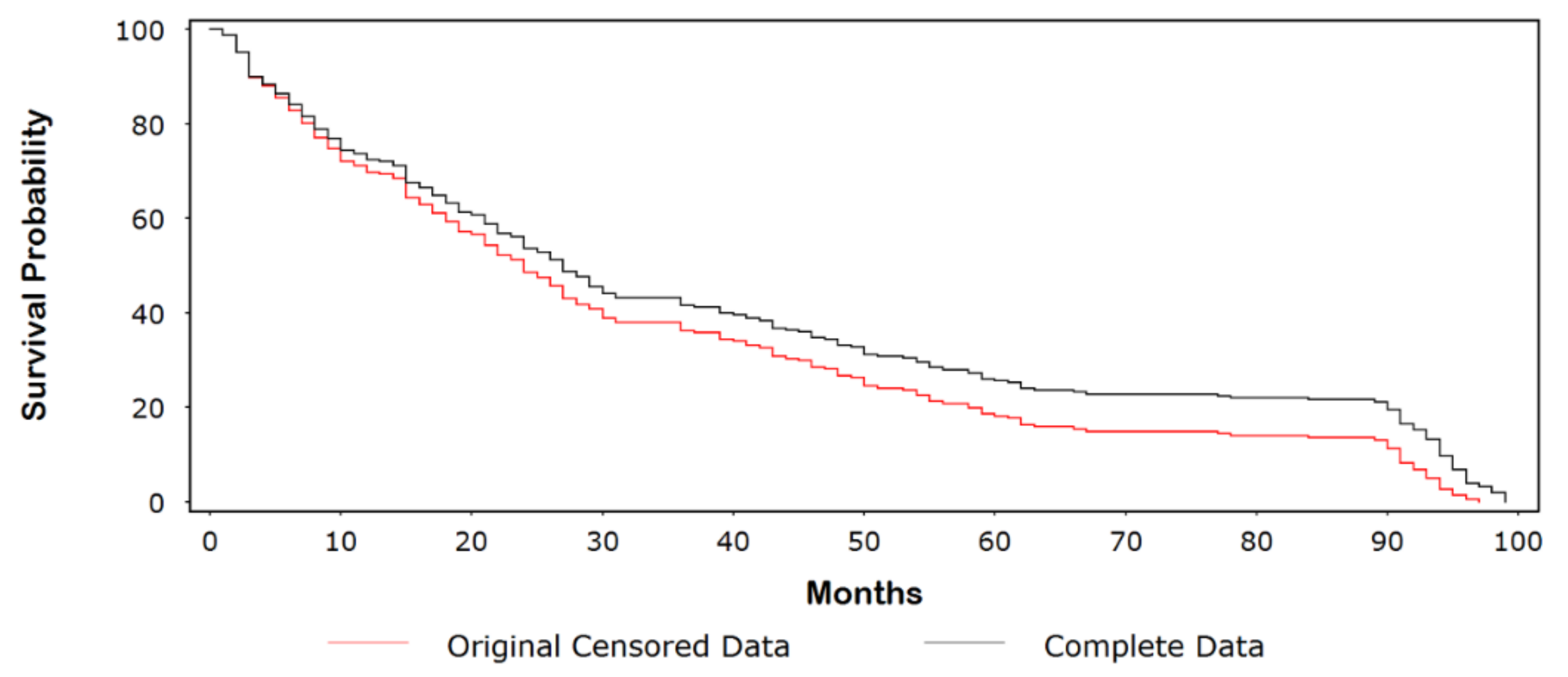
Figure 2.
Kaplan-Meir (KM) plot comparing the imputed censored data with the dataset of complete follow-up times.
Figure 2.
Kaplan-Meir (KM) plot comparing the imputed censored data with the dataset of complete follow-up times.

Figure 3.
Diagnostic plots. (A) Residuals by predicted values; (B) Studentized residuals (RStudent) by Jacobian leverages; (C) Expected raw residuals by predicted values.
Figure 3.
Diagnostic plots. (A) Residuals by predicted values; (B) Studentized residuals (RStudent) by Jacobian leverages; (C) Expected raw residuals by predicted values.

Figure 4.
Jump-point plot.
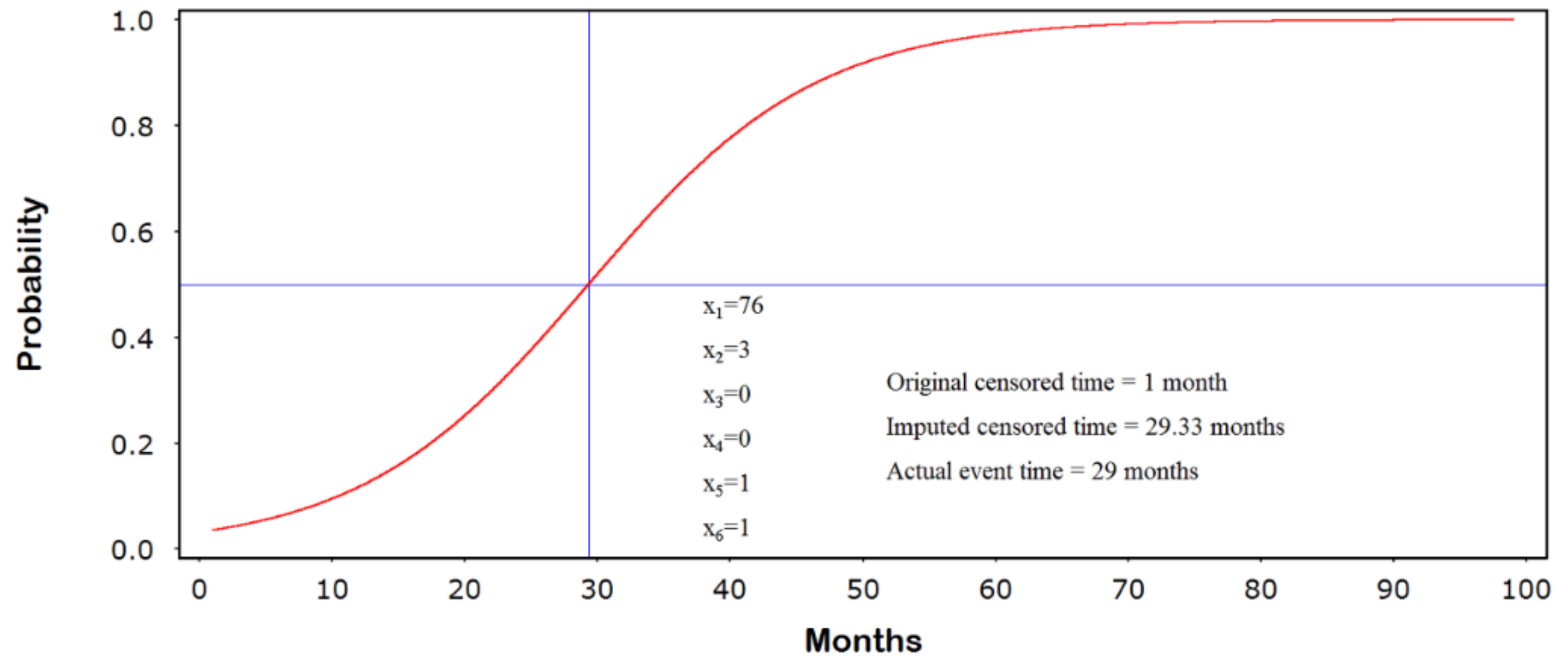
Figure 5.
SAS code used to generate jump-point plot.
© 2018 by the authors. Licensee MDPI, Basel, Switzerland. This article is an open access article distributed under the terms and conditions of the Creative Commons Attribution (CC BY) license (http://creativecommons.org/licenses/by/4.0/).
Share and Cite
MDPI and ACS Style
Efird, J.T.; Jindal, C. Using a Counting Process Method to Impute Censored Follow-Up Time Data. Int. J. Environ. Res. Public Health 2018, 15, 690. https://doi.org/10.3390/ijerph15040690
AMA Style
Efird JT, Jindal C. Using a Counting Process Method to Impute Censored Follow-Up Time Data. International Journal of Environmental Research and Public Health. 2018; 15(4):690. https://doi.org/10.3390/ijerph15040690
Chicago/Turabian StyleEfird, Jimmy T., and Charulata Jindal. 2018. "Using a Counting Process Method to Impute Censored Follow-Up Time Data" International Journal of Environmental Research and Public Health 15, no. 4: 690. https://doi.org/10.3390/ijerph15040690
Note that from the first issue of 2016, this journal uses article numbers instead of page numbers. See further details here.