A Method to Model Season of Birth as a Surrogate Environmental Risk Factor for Disease


1
Cancer Research Center of Hawaii and John A. Burns School of Medicine, 651 Ilalo Street, Biosciences Bldg. 320-B, Honolulu, HI 96813, USA
2
Public Health Sciences Division, Fred Hutchinson Cancer Research Center, Cancer Epidemiology Research Cooperative, POB 19024, 1100 Fairview Ave North, MS M4-C308, Seattle, WA 98109-1024 USA
*
Author to whom correspondence should be addressed.
Int. J. Environ. Res. Public Health 2008, 5(1), 49-53; https://doi.org/10.3390/ijerph5010049
Submission received: 9 September 2007
/
Accepted: 29 February 2008
/
Published: 30 March 2008
Abstract
:Environmental exposures, including some that vary seasonally, may play a role in the development of
many types of childhood diseases such as cancer. Those observed in children are unique in that the relevant period of
exposure is inherently limited or perhaps even specific to a very short window during prenatal development or early
infancy. As such, researchers have investigated whether specific childhood cancers are associated with season of
birth. Typically a basic method for analysis has been used, for example categorization of births into one of four
seasons, followed by simple comparisons between categories such as via logistic regression, to obtain odds ratios
(ORs), confidence intervals (CIs) and p-values. In this paper we present an alternative method, based upon an iterative
trigonometric logistic regression model used to analyze the cyclic nature of birth dates related to disease occurrence.
Disease birth-date results are presented using a sinusoidal graph with a peak date of relative risk and a single p-value
that tests whether an overall seasonal association is present. An OR and CI comparing children born in the 3-month
period around the peak to the symmetrically opposite 3-month period also can be obtained. Advantages of this
derivative-free method include ease of use, increased statistical power to detect associations, and the ability to avoid
potentially arbitrary, subjective demarcation of seasons.
Introduction
Cancer researchers have sought to demonstrate whether a link exists between season of birth and childhood diseases such as cancer [1-13]. An early narrow window of susceptibility during prenatal development [14-15] or perhaps infancy is believed to exist for childhood cancer. These periods are characterized by rapid cell growth and division and a yet undeveloped immune system. Oncogenic viruses [16-18] and chemicals [19-20] have been shown under laboratory conditions to readily induce cancers when applied during specific periods in development versus adulthood. Therefore, evidence of an association between childhood cancer and season of birth may suggest a role for a seasonally variable environmental exposure in its etiology. Exposure to infectious agents, pesticides, indoor environmental tobacco smoke and other sources of polycyclic aromatic hydrocarbons, and use of antihistamines are a few examples of environmental factors that conceivably may follow a seasonal pattern. Other factors of interest to consider in the study of childhood cancer and seasonality include harmonic variation in population mixing, diet, temperature, humidity, sunlight/photoperiod, levels of vitamin D3 and endogenous hormones.
A number of statistical tests for the analysis of harmonic data have been presented in the literature [21- 42]. This paper presents a novel and easy to use adaptation of earlier methods that is suitable for analyzing season of birth as a risk factor for diseases such as childhood cancer.
Methods
Logistic regression is used to estimate the probability for disease in relation to potential risk factors and confounding variables [43]. The technique has been widely used in epidemiologic studies, including case- control studies to examine the etiology of childhood cancer. Letting x1,…,xr denote a study participant’s values for the (r) predictor variables in a logistic regression model, the probability for disease (D) is computed as:
where are the intercept and coefficients estimated from the data using maximum likelihood methods. In a case-control study, the odds ratios (ORs) can be determined from the logistic regression model and are the exponentiated values of e by the corresponding estimated regression coefficients A p-value for a specific predictor variable may be determined by taking twice the logarithm of the ratio of the likelihood of the data under the model including the variable to the likelihood without the variable. The resulting value is compared to a statistic with 1 degree of freedom.
A predictor variable in the simplest case may be expressed as a dichotomous variable, e.g., whether birth occurred in summer. However, more complex forms may be appropriate. A variable such as date of birth (DOB, coded as an integer from 1 to 365) may be expressed as a trigonometric function [44-45]. In this example, let
where is determined iteratively by finding the value from 1 to 365 that maximizes the coefficient . The maximum 3-month seasonal period of risk is found by taking the 91.25 day-wide interval centered on . Analogously, the minimum risk period is found by taking the symmetrically opposite 3-month interval centered on . The seasonal association is visualized by plotting (i.e., harmonic displacement) against DOB over the range 1 to 365. A single p-value can be obtained as described above for this predictor variable to test whether a seasonal pattern exists. An OR for disease in the maximum versus minimum 3-month seasonal period and corresponding 95% confidence interval (CI) also may be computed, using standard methods [43]. In the case of a leap year, the 29th day of February is recoded as calendar day 59 so that the respective year consists of 365 days.
Example
Using hypothetical childhood cancer birth-date data from a case-control study (Appendix 1), we conducted analyses using the methods described above, and for comparison, the typical, more basic method to examine whether there is a seasonal pattern in children’s DOB. The identification of an underlying sinusoidal trend would be consistent with the hypothesis of a seasonally varying exposure (e.g., viruses, use of pesticides) as a possible etiologic risk factor for childhood cancer.
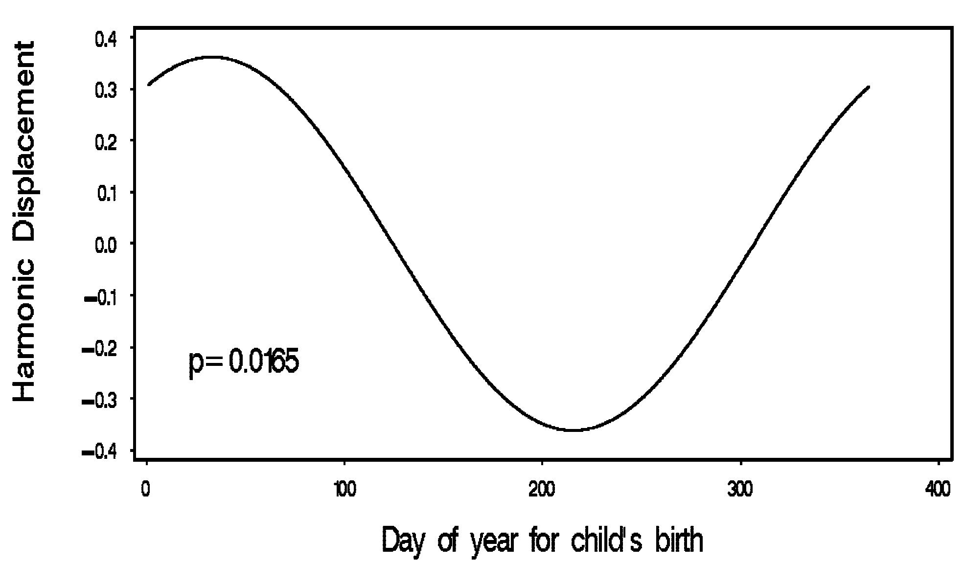
In this example, no significantly increased OR for childhood cancer (all p>0.05) was observed for pair-wise seasonal comparisons when defined in simple categorizations, here as fall (September, October, November), winter (December, January, February), spring (March, April, May), and summer (June, July, August), although the lower confidence limit for ‘winter versus summer’ was just slightly less than unity (Table 1). However, when applying equation (2) to the data in a logistic regression model, a statistically significant (p = 0.0165) seasonal pattern was observed, with peak riske occurring in early February at day 33 (Figure 1). The respective OR for childhood cancer when comparing the maximum versus minimum 3-month seasonal period was 2.2 (95% CI=1.2-4.1).

Table 1.
Odds ratios for childhood cancer by season of
child’s birth using hypothetical data (Cases n = 134,
Controls n = 261)
Table 1.
Odds ratios for childhood cancer by season of
child’s birth using hypothetical data (Cases n = 134,
Controls n = 261)
| Season of birthÞ | Odds ratio | 95% Confidence interval |
|---|---|---|
| Winter vs. Spring | 1.2 | (0.68-2.1) |
| Spring vs. Fall | 1. 0 | (0.56-1.8) |
| Winter vs. Fall | 1.2 | (0.67-2.2) |
| Winter vs. Summer | l. 8 | (0.99-3.3) |
| Spring vs. Summer | 1.5 | (0.84-2.7) |
| Fall vs. Summer | 1.5 | (0.82-2.8) |
ÞSpring = {March, April, May}; Summer = {June, July, August}; Fall = {September, October, November}; Winter = {December, January, February}.
Figure 1.
Sinusoidal logistic regression model for
hypothetical childhood cancer – birth date data.

Discussion
We have presented a simple, iterative logistic regression-based method to analyze seasonal data. The method represents a generalization of earlier trigonometric models yet is easier to apply and interpret. A novel aspect of the technique is its ability to optimally fit a sinusoidal curve to the underlying data by plotting harmonic displacement against calendar time. An additional key feature of this approach is the ability to obtain an overall p-value and an OR for disease in the “maximum versus minimum” 3-month seasonal period and a corresponding 95% CI. Whereas no single method provides a universal solution to handle harmonic data, the current method accommodates varying length of months, different populations at risk, adjustment for potentially confounding variables, and is fairly robust when used for small samples. The associated statistical test inherently will have greater family-wise power to detect a sinusoidal pattern when compared to chi-square methods or performing multiple pair-wise tests for seasonality. Analogous to a dose response relationship based upon a best-fitting monotonic model and a priori mechanism of action, multiplicity correction is not necessary for sinusoidal logistic regression because there is only one parameter and one statistical test. Furthermore, it takes into account the order of events (e.g., consecutively high/low time periods) and in contrast to pair-wise seasonal comparisons, the underlying definition of season in the current model is not arbitrary for a start and end date, but is determined via the model algorithm.
Several limitations may apply to the use of sinusoidal logistic regression. For example, parameter estimates may be biased if there is a discrepancy between observed values and values expected under the model. Accordingly, the data should be examined for goodness- of-fit using a standard procedure such as the Hosmer- Lemeshow test [46]. Erroneous results may occur in the case of multiple within-year cycles or competing out-of- phase cycles resulting in a cancelling of effects (e.g., opposing seasonal effects by histologic subgroup). A minor modification can be made to the sinusoidal function to allow for multiple cycles [25-26, 34, 40]. For example, a lunar cycle having multiple peaks per year may be modeled by substituting “365” in the denominator of equation (2) with “29.53” (i.e., the number of days in the lunar cycle). When appropriate, stratification is advised in the latter situation as a means to minimize “cancelling of effects.” Further, the lack of a seasonal effect does not necessarily rule out the etiologic importance of putative risk factors that vary in the environment seasonally. Conversely, the seasonal association of a specific risk factor with childhood cancer does not necessarily imply causality. As with any statistical test, the results of this method should be carefully interpreted in light of underlying limitations and biologic plausibility.
Acknowledgements
This manuscript was made possible by grant numbers P20 MD000173 from NCMHD and G12RR003061 from NCRR. Its contents are solely the responsibility of the authors. Dr. Elizabeth Holly, Ph.D. offered valuable comments during the writing of this manuscript and her knowledge and insight has been greatly appreciated.
Appendix 1: Hypothetical case-control data (Cases n=134, Controls n=261)
| Day of birth | No. of cases | No. of controls | Day of birth | No. of cases | No. of controls | Day of birth | No. of cases | No. of controls | Day of birth | No. of cases | No. of controls | Day of birth | No. of cases | No. of controls |
| 1 | 1 | 1 | 77 | 1 | 0 | 139 | 0 | 1 | 212 | 0 | 2 | 288 | 0 | 1 |
| 3 | 1 | 2 | 78 | 1 | 0 | 140 | 1 | 2 | 213 | 0 | 1 | 289 | 1 | 0 |
| 4 | 1 | 0 | 79 | 1 | 1 | 141 | 0 | 3 | 214 | 1 | 0 | 290 | 1 | 0 |
| 5 | 0 | 2 | 80 | 1 | 0 | 142 | 1 | 1 | 215 | 0 | 2 | 291 | 0 | 1 |
| 6 | 0 | 1 | 81 | 0 | 1 | 143 | 1 | 1 | 216 | 0 | 2 | 293 | 1 | 0 |
| 7 | 0 | 1 | 83 | 0 | 1 | 144 | 0 | 2 | 217 | 0 | 1 | 294 | 0 | 1 |
| 8 | 2 | 1 | 85 | 0 | 1 | 146 | 2 | 0 | 221 | 1 | 1 | 296 | 1 | 0 |
| 12 | 0 | 2 | 86 | 1 | 1 | 147 | 0 | 2 | 223 | 2 | 1 | 297 | 1 | 4 |
| 15 | 1 | 1 | 87 | 0 | 1 | 148 | 0 | 1 | 224 | 0 | 1 | 298 | 0 | 1 |
| 17 | 0 | 2 | 88 | 0 | 2 | 150 | 0 | 1 | 225 | 0 | 1 | 299 | 1 | 2 |
| 18 | 2 | 0 | 89 | 0 | 2 | 152 | 0 | 1 | 226 | 3 | 3 | 300 | 1 | 0 |
| 19 | 1 | 0 | 90 | 1 | 0 | 154 | 1 | 1 | 227 | 0 | 2 | 301 | 0 | 1 |
| 21 | 1 | 1 | 91 | 1 | 0 | 155 | 0 | 1 | 228 | 0 | 1 | 303 | 1 | 0 |
| 22 | 1 | 1 | 92 | 0 | 2 | 157 | 1 | 0 | 230 | 0 | 1 | 304 | 2 | 0 |
| 23 | 1 | 1 | 93 | 1 | 1 | 159 | 0 | 2 | 231 | 1 | 2 | 305 | 0 | 1 |
| 24 | 1 | 0 | 94 | 2 | 1 | 160 | 0 | 1 | 232 | 0 | 1 | 306 | 0 | 1 |
| 26 | 0 | 1 | 96 | 0 | 1 | 161 | 0 | 1 | 234 | 1 | 1 | 307 | 0 | 3 |
| 27 | 1 | 1 | 97 | 1 | 1 | 164 | 1 | 0 | 235 | 0 | 2 | 308 | 0 | 1 |
| 29 | 0 | 1 | 99 | 1 | 0 | 166 | 0 | 2 | 236 | 0 | 2 | 309 | 1 | 2 |
| 32 | 0 | 2 | 100 | 0 | 2 | 167 | 1 | 0 | 237 | 1 | 1 | 311 | 1 | 2 |
| 33 | 1 | 1 | 102 | 1 | 2 | 168 | 2 | 0 | 239 | 0 | 1 | 312 | 1 | 0 |
| 35 | 1 | 0 | 103 | 0 | 1 | 169 | 0 | 1 | 240 | 0 | 1 | 313 | 1 | 2 |
| 36 | 0 | 1 | 107 | 1 | 0 | 170 | 0 | 1 | 242 | 0 | 2 | 314 | 1 | 1 |
| 39 | 2 | 2 | 108 | 0 | 1 | 172 | 0 | 1 | 245 | 0 | 1 | 316 | 1 | 0 |
| 40 | 1 | 1 | 109 | 1 | 1 | 174 | 1 | 1 | 246 | 0 | 1 | 320 | 0 | 1 |
| 42 | 1 | 1 | 110 | 1 | 0 | 175 | 1 | 2 | 248 | 2 | 0 | 322 | 2 | 1 |
| 43 | 0 | 2 | 111 | 0 | 4 | 176 | 0 | 1 | 249 | 0 | 1 | 323 | 1 | 0 |
| 45 | 0 | 1 | 112 | 1 | 1 | 177 | 0 | 1 | 251 | 2 | 3 | 324 | 1 | 1 |
| 46 | 1 | 0 | 113 | 0 | 1 | 179 | 2 | 0 | 252 | 0 | 1 | 325 | 0 | 1 |
| 47 | 1 | 1 | 114 | 1 | 1 | 180 | 0 | 1 | 253 | 1 | 2 | 327 | 0 | 1 |
| 48 | 0 | 1 | 115 | 0 | 1 | 182 | 0 | 2 | 255 | 0 | 1 | 328 | 1 | 0 |
| 49 | 0 | 1 | 116 | 1 | 0 | 184 | 1 | 0 | 256 | 1 | 2 | 329 | 0 | 1 |
| 50 | 1 | 0 | 117 | 1 | 0 | 186 | 1 | 1 | 257 | 0 | 1 | 331 | 1 | 0 |
| 51 | 0 | 1 | 118 | 0 | 1 | 187 | 0 | 2 | 262 | 1 | 0 | 336 | 1 | 0 |
| 53 | 1 | 0 | 119 | 0 | 2 | 188 | 0 | 2 | 263 | 1 | 1 | 338 | 1 | 1 |
| 54 | 1 | 1 | 120 | 1 | 0 | 190 | 0 | 2 | 264 | 0 | 1 | 340 | 0 | 1 |
| 56 | 1 | 0 | 122 | 1 | 1 | 191 | 0 | 1 | 265 | 0 | 2 | 341 | 0 | 1 |
| 57 | 1 | 1 | 123 | 0 | 1 | 194 | 0 | 1 | 266 | 1 | 1 | 342 | 0 | 1 |
| 58 | 1 | 0 | 124 | 0 | 2 | 195 | 0 | 1 | 267 | 0 | 1 | 345 | 0 | 1 |
| 59 | 1 | 1 | 125 | 1 | 0 | 196 | 0 | 2 | 269 | 1 | 0 | 346 | 1 | 1 |
| 60 | 0 | 2 | 126 | 2 | 0 | 197 | 1 | 0 | 270 | 0 | 1 | 347 | 0 | 1 |
| 62 | 2 | 0 | 127 | 0 | 1 | 198 | 1 | 1 | 273 | 0 | 1 | 349 | 1 | 0 |
| 63 | 0 | 1 | 129 | 0 | 1 | 199 | 0 | 1 | 274 | 0 | 1 | 351 | 0 | 1 |
| 66 | 1 | 0 | 130 | 1 | 0 | 200 | 1 | 1 | 276 | 0 | 1 | 356 | 0 | 2 |
| 68 | 0 | 2 | 131 | 0 | 2 | 202 | 1 | 1 | 277 | 0 | 2 | 358 | 0 | 1 |
| 69 | 1 | 2 | 132 | 1 | 0 | 203 | 0 | 2 | 278 | 0 | 1 | 359 | 2 | 1 |
| 70 | 0 | 1 | 133 | 0 | 1 | 204 | 1 | 1 | 279 | 0 | 1 | 361 | 0 | 1 |
| 71 | 1 | 0 | 135 | 1 | 0 | 208 | 0 | 1 | 282 | 1 | 2 | 362 | 0 | 3 |
| 73 | 0 | 1 | 136 | 0 | 2 | 209 | 0 | 2 | 284 | 0 | 1 | 364 | 0 | 1 |
| 75 | 0 | 1 | 138 | 0 | 1 | 210 | 0 | 1 | 287 | 0 | 1 | 365 | 1 | 1 |
References
- Ederer, F.; Miller, R.; Scotto, J; Bailar, J.: Birth- month and infant cancer mortality. Lancet, 1965, 7404, 185-186.
- Stark, C.; Mantel, N. Temporal-spatial distribution of birth dates for Michigan children with leukemia. Cancer Res, 1967, 27, 1749-1775. [Google Scholar]
- Yamakawa, Y.; Fukui, M.; Kinoshita, K.; Ohgami, S.; Kitamura K.: Seasonal variation in incidence of cerebellar medulloblastoma by month of birth. Fukuoka Igaku Zasshi (Hukuoka Acta Medica), 1979, 70, 295-300.
- Meltzer, A.; Spitz, M.; Johnson, C.; Culbert, S.: Season-of-birth and acute leukemia of infancy. Chronobiol Int, 1989, 6, 285-289.
- Meltzer, A.; Annegers, F.; Spitz, M.: Month-of-birth and incidence of acute lymphoblastic leukemia in children. Leuk Lymphoma, 1996, 23, 85-92.
- Alexander, F.; Boyle, P.; Carli, P.; Coebergh, J.; Draper, G.; Ekbom, A.; Levi, F.; McKinney, P.; McWhirter, W.; Magnani, C.; Michaelis, J.; Olsen, J.; Peris-Bonet, R.; Petridou, E.; Pukkala, E.; Vatten, L. 1998: Spatial temporal patterns in childhood leukaemia: further evidence for an infectious origin. EUROCLUS project. Br J Cancer, 1998, 77, 812- 817.
- Heuch, J.; Heuch, I.; Akslen, L.; Kvale, G.: Risk of primary childhood brain tumors related to birth characteristics: a Norwegian prospective study. Int J Cancer, 1998, 77, 498-503.
- Feltbower, R.; Pearce, M.; Dickinson, H.; Parker, L.; McKinney, P.: Seasonality of birth for cancer in northern England, UK. Paediatr Perinat Epidemiol, 2001, 15, 338-345.
- Higgins, C.; dos-Santos-Silva, I.; Stiller, C.; Swerdlow, A.: Season of birth and diagnosis of children with leukaemia: an analysis of over 15000 UK cases occurring from 1953-95. Br J Cancer, 2001, 84, 406-412.
- Sorensen, H.; Olsen, J.; Rothman, K.: Seasonal variation in month of birth and diagnosis of early childhood acute lymphoblastic leukemia. JAMA, 2001, 285, 168-169.
- McNally, R.; Cairns, D.; Eden, O.; Alexander, F.; Talyor, G.; Kelsey, A.; Birch, J.: An infectious aetiology for childhood brain tumours? Evidence from space-time clustering and seasonality analyses. Br J Cancer, 2002, 86, 1070-1077.
- Halperin, E.; Miranda, M.; Watson, D.; George, S.; Stanberry, M.: Medulloblastoma and birth date: evaluating three U.S. data sets. Arch Environ Health, 2004, 59, 26-30.
- Mainio, A.; Hakko, H.; Koivukangas, J.; Niemela, A.: Winter birth in association with a risk of brain tumor among a Finnish patient population. Neuroepidemiology, 2006, 27, 57-60.
- Rice, J.; Ward, J.: Age dependence of susceptibility to carcinogenesis in the nervous system. Ann NY Acad Sci, 1982, 381, 274-289.
- Alexandrov, V.; Aiello C.; Rossi L.: Modifying factors in prenatal carcinogenesis. In Vivo, 1990, 4, 327-336.
- Sanders, F.: Experimental carcinogenesis: Induction of multiple tumors by viruses. Cancer, 1977, 40, 1841-1844.
- Zu Rhein, G.; Varakis, J.: Perinatal induction of medulloblastomas in Syrian golden hamsters by a human polyoma virus (JC). Natl Cancer Inst Monogr, 1979, 51, 205-208.
- Varakis, J.; ZuRhein, G.; Padgett, B.; Walker, D.: Induction of peripheral neuroblastomas in Syrian hamsters after injection as neonates with JC virus, a human poloma virus. Cancer Res, 1978, 38, 1718- 1722.
- Druckrey, H.; Ivankovic, S.; Preussmann, R.: Teratogenic and carcinogenic effects in the offspring after single injection of ethylnitrosourea to pregnant rats. Nature, 1966, 210, 1378-1379.
- Wechsler, W.; Kleihues, P.; Matsumoto, S.; Zulch, K.; Ivankovic, S.; Preussmann, R.; Druckrey, H.: Pathology of experimental neurogenic tumors chemically induced during prenatal and postnatal life. Ann NY Acad Sci, 1969, 159, 360-408.
- Stutvoet, H.: Seasonal birth frequencies in parameters. Acta Genet Stat Med, 1951, 2, 177-192. 2.
- Jonckheere, A.: A distribution-free k-sample test against ordered alternatives. Biometrika, 1954, 41, 133-145.
- Edwards, J.: The recognition and estimation of cyclic trends. Ann Hum Genet Lond, 1961, 25, 83-87.
- Hewitt, D.; Milner, J.; Csima, A.; Pakula, A.: On Edwards’ criterion of seasonality and a non- parametric alternative. Brit J Prev Soc Med, 1971, 25, 174-176.
- Thomas, J.; Wallis, K.: Seasonal variation in regression analysis. J R Statist Soc A, 1971, 134, 57-72.
- Cave, D.; Freedman, L.: Seasonal variation in the clinical presentation of Crohn’s disease and ulcerative colitis. Int J Epidemiol, 1975, 4, 317-320.
- Walter, S.; Elwood, J.: A test for seasonality of events with a variable population at risk. Brit J Prev Soc Med, 1975, 29, 18-21.
- St. Leger, A.: Comparison of two tests for seasonality in epidemiology data. Appl Statist, 1976, 25, 280- 286.
- Roger, J.: A significance test for cyclic trends in incidence data. Biometrika, 1977, 64, 152-155.
- Becker, S.: Seasonal patterns of fertility measures: theory and data. JASA, 1981, 76, 249-259.
- Marrero, O.: The performance of several statistical tests for seasonality in monthly data. J Statist Comput Simul, 1983, 17, 275-296.
- Nonaka, K.; Miura, T.: Principles in methods of epidemiological studies on birth seasonality. Prog Biometerology, 1987, 6, 13-24.
- Jones, R.; Ford, P.; Hamman, R.: Seasonality comparisons among groups using incidence data. Biometrics, 1988, 44, 1131-44.
- Bound, J.; Harvey, P.; Francis, B.: Seasonal prevalence of major congenital malformations in the Fylde of Lancashire 1957-1981. J. Epidemiol Community Health, 1989, 43, 330-342.
- Eubank, R.; Speckman, P.: Curve fitting by polynomial-trigonometric regression. Biometrika, 1990, 77, 1-9.
- Reijneveld, S.: The choice of a statistic for testing hypotheses regarding seasonality. Am J Phys Anthropol, 1990, 83, 181-184.
- Lam, D.; Miron, D.: Seasonality of births in human populations. Soc Biol, 1991, 38, 51-78.
- Lam, D.; Miron, J.; Riley, A.: Modeling seasonality in fecundability conceptions, and birth. Demography, 1994, 31, 321-346.
- Woodhouse, P.; Khaw, K.: Seasonal variations of plasma fibrinogen and factor VII activity in the elderly: Winter infections and deaths from cardiovascular disease. Lancet, 1994, 343, 435-439.
- Stolwijk, A.; Straatman, H.; Zielhuis, G. Studying seasonality by using sine and cosine functions in regression analysis. J Epidemiol Community Health, 1999, 53, 235-238.
- Eriksson, A.; Fellman, J.: Seasonal variation of livebirths, stillbirths, extramarital births and twin maternities in Switzerland. Twin Res, 2000, 3, 289-201.
- Fellman, J.; Erikkson, A.: Statistical analysis of the seasonal variation in demographic data. Human Biol, 2000, 72, 851-876.
- Kelsey, J.; Whittemore, A.; Evans, A.; Thompson, W.: Methods in Observational Epidemiology. Oxford University Press: New York, 1996; pp. 1-412.
- Beckett, L.: Personal communication, 1987.
- Chodick, G.; Shalev, V.; Goren, I.; Inskip, P.: Seasonality in birth weight in Israel: new evidence suggests several global patterns and different etiologies. Ann Epidemiol, 2007, 17, 440-446.
- Hosmer, D.; Lemeshow, S.: Applied Logistic Regression. New York, John Wiley & Sons, Inc.: New York, 2000; pp. 1-392.
Publisher’s Note: MDPI stays neutral with regard to jurisdictional claims in published maps and institutional affiliations. |
© 2008 by the authors. Licensee MDPI, Basel, Switzerland. This article is an open access article distributed under the terms and conditions of the Creative Commons Attribution (CC BY) license (https://creativecommons.org/licenses/by/4.0/).
Share and Cite
MDPI and ACS Style
Efird, J.T.; Nielsen, S.S. A Method to Model Season of Birth as a Surrogate Environmental Risk Factor for Disease. Int. J. Environ. Res. Public Health 2008, 5, 49-53. https://doi.org/10.3390/ijerph5010049
AMA Style
Efird JT, Nielsen SS. A Method to Model Season of Birth as a Surrogate Environmental Risk Factor for Disease. International Journal of Environmental Research and Public Health. 2008; 5(1):49-53. https://doi.org/10.3390/ijerph5010049
Chicago/Turabian StyleEfird, Jimmy Thomas, and Susan Searles Nielsen. 2008. "A Method to Model Season of Birth as a Surrogate Environmental Risk Factor for Disease" International Journal of Environmental Research and Public Health 5, no. 1: 49-53. https://doi.org/10.3390/ijerph5010049