Review

Usefulness of Mendelian Randomization in Observational Epidemiology

University Institute of Social and Preventive Medicine, Rue du Bugnon 17, 1005 Lausanne, Switzerland
*
Author to whom correspondence should be addressed.
Int. J. Environ. Res. Public Health 2010, 7(3), 711-728; https://doi.org/10.3390/ijerph7030711
Submission received: 29 December 2009 / Accepted: 16 February 2010 / Published: 26 February 2010
(This article belongs to the Special Issue Advances in Epidemiology)

Abstract

:
Mendelian randomization refers to the random allocation of alleles at the time of gamete formation. In observational epidemiology, this refers to the use of genetic variants to estimate a causal effect between a modifiable risk factor and an outcome of interest. In this review, we recall the principles of a “Mendelian randomization” approach in observational epidemiology, which is based on the technique of instrumental variables; we provide simulations and an example based on real data to demonstrate its implications; we present the results of a systematic search on original articles having used this approach; and we discuss some limitations of this approach in view of what has been found so far.

Graphical Abstract

1. Introduction

Observational studies have brought important insight into disease etiology. During the past decade however, the validity of observational studies has been questioned [1]. This is due to the fact that the role of selected risk, or protective, factors identified via observational studies could not be confirmed by subsequent large randomized controlled trials. For instance, hormonal replacement therapy appeared to protect women against coronary heart disease in observational studies [2], whereas randomized trials showed no such protection [3]. Other examples are given by antioxidant vitamin supplementation [46].
One cannot, for ethical and technical reasons, randomize risk factors using controlled trials in humans. The identification of risk factors therefore relies on observational studies, which are prone to spurious results due to confounding factors, reverse causation, and/or selection biases [7]. As a consequence, it is difficult to firmly establish causal relationships between risk factors and disease. Most common diseases (e.g., cancer, cardiovascular disease, etc.) are complex and are influenced by multiple risk factors that may be correlated with each other. In this context, each factor is expected to have a small influence on disease risk. Epidemiologists have the hard task to determine whether a putative risk factor is causally related to a specific disease, independently of all other risk factors. A promising approach to help epidemiologists in this task is Mendelian randomization. In this review, we first recall the principles of a “Mendelian randomization” approach in observational epidemiology (Section 2), we then provide some technical explanation of the method of instrumental variable (Section 3), followed by simulations and an example with real data (Section 4). We then present the results of a systematic search on original articles having used this approach (Section 5), discuss its limitations (Section 6) and present concluding remarks (Section 7).

2. Mendelian Randomization in Observation Epidemiology

Mendelian randomization refers to the random allocation of alleles at the time of gamete formation. A specific genotype carried by a person therefore results from two such randomized transmissions, one from the paternally inherited allele and the other from the maternally inherited allele. A logical consequence of these randomizations is that genotypes are not expected to be associated with known (measurable or not) or unknown confounders for any outcome of interest, except those lying on the causal pathway between the genotype and the outcome. This should hence allow analyzing the genotype-risk factor association and the genotype-outcome association in an unconfounded manner. By combining appropriately the results of these two analyses, one can get an estimate of the risk factor-outcome association, which is itself not confounded. This is analogous to randomized controlled trials (of sufficient sample size), in which the random allocation of treatment (or preventive measure) is expected to lead to an even distribution of (known or unknown) confounding factors across each groups. The term “Mendelian randomization” is now frequently used in observational epidemiology to refer to the use of genetic variants to estimate a causal effect between a specific modifiable risk factor and a trait/disease of interest. The idea is to overcome some of the problems encountered in observational epidemiology, such as residual confounding and reverse causation, by taking advantage of the natural random allocation of alleles during meiosis [8].
We here provide an example to illustrate this approach. The aldehyde dehydrogenase 2 (ALDH2) gene encodes the enzyme aldehyde dehydrogenase, which catalyzes the chemical transformation from acetaldehyde to acetic acid. Carriers of the ALDH2 *2*2 genotype have reduced alcohol consumption because of adverse reactions (facial flush, headache, nausea and drowsiness) due to acetaldehyde accumulation. This fact has been used to show that alcohol intake increases the risk of esophageal cancer [9] or head and neck cancer [10], which is consistent with the findings from observational studies. Whereas reported alcohol consumption may be subject to measurement errors, ALDH2 genotypes can be measured accurately, are present since birth, result from the random allocation of the paternally and maternally inherited alleles, are strongly associated with alcohol consumption, and therefore provide a unique opportunity to assess, in an unconfounded manner, the risk of disease associated with alcohol consumption. As we shall discuss in Section 6, such an approach - although appealing - also raises some methodological issues.
Historically, the first description of the concept of Mendelian randomization in observational epidemiology is attributed to Katan [11], who suggested to use the APOE gene to infer causality between cholesterol and cancer. The concept was further developed by Davey Smith and Ebrahim [7,8,12,13], who have shown that the causal effect of a risk factor (X) on an outcome (Y) can be estimated by combining the effects of a genetic variant (Z) on X and on Y, provided that certain assumptions are met (see Figure 1). Thomas and Conti [14] have shown that the Mendelian randomization approach was in fact an application of the instrumental variable approach, which had been used since more than 70 years by econometricians. Wehby et al. have recently advocated that the term “Mendelian randomization” should be replaced by “instrumental variable analysis with genetic instruments” [15]. We tend to agree with this latter statement after having reviewed the medical literature and observed that the term “Mendelian randomization” was used with different meanings by different researchers, which might be confusing.

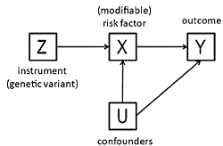
3. The Method of Instrumental Variables

We consider the case where an association between a continuous (or binary) modifiable exposure X and a continuous response Y is measured via a beta coefficient in a linear regression, defined as the average increase in Y when X is increased by one unit (respectively, when changing the category of X if the exposure is binary). When observing such an association in epidemiological research, however, it is often difficult to determine which of the two variables (X or Y) is the cause and which the effect, or whether a third variable (a confounder, U) related to both variables is responsible for the observed association. Moreover, measurement error could attenuate the beta coefficient. Thus, it is not obvious how a significant non-zero (e.g., positive) beta coefficient obtained from a classical (ordinary) least squares estimate should be interpreted. Here are five possible interpretations (among many others):
  • The beta coefficient is a consistent estimate of the causal effect of X on Y.
  • The beta coefficient is actually underestimating the true causal effect of X on Y because of measurement error.
  • The beta coefficient is overestimating the true causal effect of X on Y because of the presence of a confounder which is positively related to both X and Y.
  • The non-zero beta coefficient is entirely due to the presence of a confounder which is related to both X and Y: in fact there is no causal effect of X on Y.
  • The beta coefficient is non-zero because of a causal effect of Y on X, not of X on Y (i.e., reverse causation).
In other words, if the interest lies in assessing “the causal effect of X on Y”, i.e., the effect that would be observed if one could intervene and change someone’s X level by one unit, leaving other characteristics unchanged, no definitive conclusion can be drawn from such an analysis. We shall see below, illustrated in the context described by Figure 1, how the method of instrumental variables can help in this regard.
A linear model (consistent with Figure 1) is given by:
Y = α 1 + β 1 X + γ 1 U
where β1 is the causal effect of X on Y and where γ1U plays the role of the error term, U being some unobserved confounder. Whenever X is correlated with the error term (see Figure 1), the expectation of the least squares estimate of the slope in this model, which we denote by β 1 L S, will be different from β1.
The method of instrumental variables has been proposed to correct for the bias of the least squares estimate. For this, we need to have at our disposal an “instrumental variable”, or instrument Z, for the time being continuous or binary, satisfying the following conditions: (1) Z is correlated with X, (2) Z is independent from U, and (3) Z and Y are independent given X and U. Note that the former of these conditions is verifiable from the data, whereas the latter two are largely not.
A second linear model (consistent with Figure 1) is then as follows:
X = α 2 + β 2 Z + γ 2 U
where γ2U plays the role of the error term in the model. Since Z is by assumption uncorrelated with this error term, the coefficients of this second model are estimated without bias by least squares. Note that the first model can be rewritten as:
Y = α 1 + β 1 α 2 + β 1 β 2 Z + ( γ 1 + β 1 γ 2 ) U
Denoting α3 = α1 + β1α2, β3 = β1β2 and γ3 = γ1 + β1γ2, we obtain hence a third linear model:
Y = α 3 + β 3 Z + γ 3 U
where γ3U is the error term. Since Z is by assumption uncorrelated with this error term, the coefficients of this third model are also estimated without bias by least squares.
At the end, the parameters of the first model can be consistently estimated using relationships α1 = α3β1α2 and β1 = β3/β2, the denominator β2 being non zero by assumption. In particular, the instrumental variable (IV) estimate of the causal effect β1 in the first model is the quotient of the two least squares estimates of slope parameters β3 and β2 in the third and second models. Since the expectation of a quotient of two estimates is asymptotically equal to the quotient of the expectations of these estimates, the IV estimates are asymptotically unbiased, but they may be biased in finite samples.
Asymptotically, the IV estimates are normally distributed and explicit formulae for the standard errors are available, enabling to calculate confidence intervals and to test for the nullity of the causal effect β1 in the first model (as calculated e.g., with the ivregress 2sls command implemented in Stata 10.0). The standard error of the estimates will depend, among others, on the percentage of explained variance in the second model (itself related to the percentage of explained variance in the third model). If this percentage is low, the instrument is said to be weak, the standard errors will be large and the test above will have low power. Moreover, the bias of the IV estimates is typically larger, and the asymptotic normal distribution of the IV estimates may be a poor approximation to the true distribution, when the instrument is weak, the inference being then unreliable [17]. In practice, an instrument is said to be weak if the F-statistics for testing the nullity of parameter β2 in the second model is inferior to 10 [18].
Another equivalent way to calculate the IV estimates (but without their standard errors!) is to perform a “two-stage least squares”, regressing X on Z in a first stage (this is the second model above), and regressing Y on the obtained fitted values (Z) in a second stage. The method of instrumental variables can be readily extended to the case of several instrumental variables (and therefore to the case of a qualitative instrument), which may be useful to improve the precision of the instrumental variable estimate. One can also adjust for additional covariates in each of the above models.
In addition to test for the nullity of the causal effect β1, one may also test for the absence of correlation between X and the error term in the first model, implying the equality of the parameters β1 and β 1 L S, using the Durbin-Wu-Hausman test. This may be of some interest when comparing several candidate models which may have generated the data (see the simulations below).

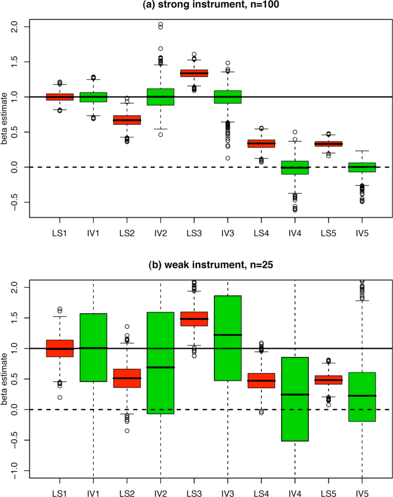
4. Simulations and Example

To illustrate that the method of instrumental variable is effective, we simulated data from five models consistent with the five above-mentioned interpretations (Table 1). In each case, we simulated an instrument Z satisfying the conditions. For simplicity, we took all intercepts in these models to be 0, all slopes to be 1, and the variables which were generated at each step were taken to be N(0,1), i.e., normally distributed with mean 0 and variance 1.
The causal effect of X on Y that we are looking for is β1 = 1 under the first three models, and is β1 = 0 under the last two models. Boxplots of the least squares (LS) estimates and of the instrumental variable (IV) estimates of parameter β1 obtained from 1,000 samples of size n = 100 under each of the five models are shown on the top panel of Figure 2. The LS estimate is unbiased under the first model, is consistently too small under the second model, and is consistently too large under the last three models. By contrast, the IV estimate is almost unbiased under each of the five models, which is actually remarkable. One can also notice that the IV estimate shows a higher variability than the LS estimate, which is the price to pay for correcting the bias of the latter. The Durbin-Wu-Hausman test was significant in 4.1% (which was close to the nominal 5% level) of the samples generated from the first model, for which β 1 = β 1 L S holds, in 66% of the samples generated from the second model, for which β 1 > β 1 L S holds, and in 88%, 90% and 100% from the samples generated respectively from the third, fourth and fifth models, for which β 1 < β 1 L S holds.
To provide an idea of what may happen when using a weak instrument, we considered the same five models, but the slopes involving Z were set to 0.25 (instead of 1) in each model. In addition, we reduced the sample size to n = 25. Under that setting, the F-statistic in the first stage regression was smaller than 10 in more than 95% of the generated samples. Boxplots of the estimates obtained from 1,000 samples are shown on the bottom panel of Figure 2. One can see that the variance of the IV estimates dramatically increased (compared to the top panel), while some non-negligible bias appeared.
We next provide an example with real data to illustrate that the method of instrumental variable is able to correct for the bias of least squares in a case of reverse causation. We used the 1,268 participants of the population-based CoLaus study [19], who reported that they consumed alcohol regularly and who had available data for genetic markers located with the gammaglutamyl transferase 1 (GGT1) gene as well as circulating GGT levels (X). CoLaus participants have been genotyped using the Affymetrix 500 K chip, alcohol consumption was assessed using a standardized questionnaire and coded in units of alcohol per week, and GGT levels were measured using standard procedures as previously described [19]. As we were interested in exploring an example of reverse causation, we chose Y to be the reported alcohol consumption and tested whether circulating GGT (X) could cause alcohol consumption (which we know is the opposite of the reality) using the best GGT1 marker as our instrument (Z). Rs2017869 explained 1.12% of circulating GGT levels. The parameter β1 was estimated using least squares and the method of instrumental variables (the latter with the ivregress 2sls command implemented in Stata 10.0). The LS estimate (95%CI) was 5.53 (4.73;6.33) mmol/L per risk allele. The IV estimate (95%CI) was −4.60 (−13.82; 4.63) mmol/L per risk allele, which was significantly different from the LS estimate in a Durbin-Wu-Hausman test (P = 0.03), and not significantly different from zero. Thus, while the result provided by least squares was highly significant, the instrumental variable approach did not show any evidence for a positive causal association of GGT on alcohol consumption.

5. Review of Observational Studies Using Mendelian Randomization

We searched MEDLINE using the following «Mendelian randomization» OR “Mendelian randomisation”, which retrieved 99 citations (January 13, 2009). We acknowledge that this search strategy might not have retrieved all publications using the concept of Mendelian randomization, but it should provide a good overview of what has been published. The aim was to identify original articles reporting results from an observational study using a Mendelian randomization approach. We also searched references from review papers and original articles, as well as citations of these papers.
We identified 23 studies with a dichotomous trait as the outcome of interest (Table 2) and 15 studies with a continuous trait as the outcome of interest (Table 3). Considering that the instrumental variable approach has been introduced, and is well understood, for a continuous outcome, it was a bit of a surprise to find that a majority of studies in fact applied this method to a dichotomous outcome (using non-linear models and odds-ratios to quantify the associations, for which the method has not been quite validated, see also the next section). Thirteen out of 23 studies focusing on binary outcomes (Table 2) reported results compatible with a causal association. Most studies were in the field of cardiovascular epidemiology and cancer epidemiology. For continuous outcomes (Table 3), half of studies reported some evidence for causality and most studies were in the field of cardiovascular epidemiology. Most instruments reported in these studies were weak (Figure 3). We also found many studies that claimed to use a Mendelian randomization approach although they only analyzed the genotype-outcome association, hence focusing on hypothesis testing (i.e., to confirm or disprove causality). Yet, what is of interest in the Mendelian randomization approach is to estimate the causal effect of X, the modifiable factor, on Y and not simply the association between Z and Y.

6. Some Limitations of Mendelian Randomization

In order to use Mendelian randomization to infer causality in observational epidemiology, numerous conditions need to be fulfilled [13,5557]. A major limitation of this approach is that it is difficult, in practice, to meet al.l these conditions for a given risk factor—outcome association. To fulfill the first condition, Z and X should be correlated (genetic instruments for common complex diseases are typically quite weak). This indirectly implies that there is some level of allelic homogeneity (i.e., common variants rather than rare variants). Note that for many exposures, no suitable genetic instrument is available. The second and third conditions are the problematic ones. They state that Z is (marginally) independent from all potential confounders U, and that Z and Y are independent conditionally on X and U [57]. In an excellent introduction to Mendelian randomization, Didelez and Sheehan [58] wrote that “if we know a gene closely linked to the phenotype without direct effect on the disease, it can often be reasonably assumed that the gene is not itself associated with any confounding factors”. See however Section 7 of that paper for situations in which these conditions are not satisfied. Mendel’s second law (i.e., the law of independent assortment of alleles at the time of gamete formation) is not always true in that genetic variants located on the same chromosome, particularly for close loci, do not segregate independently (i.e., they are linked), as detailed in Lawlor et al. [13]. At the population level, such physical linkage patterns result in linkage disequilibrium, i.e., correlations between alleles at nearly loci. In genetic epidemiology, the second condition implies, among others, that there should be no confounding due to linkage disequilibrium (i.e., instrument Z should not be correlated with other genetic variants having an effect on the outcome of interest, Y) [13]. However, the instrument Z does not necessarily need to be causally associated with X, in that another genetic variant associated to both Z and X might be the true causal variant [13]. Similarly, population stratification, i.e., the existence of population subgroups with different allele frequencies and outcome distributions, may violate this second condition as well. In the Mendelian randomization context, confounding may exist if the subgroups (these often correspond to ethnic groups) are associated to both Z and Y [13].
Also, there should be no pleiotropy, (i.e., Z having multiple effects, which do not pass through X). This is however only a problem if the other functions of Z are associated to Y [13]. There should be no canalization (also called developmental compensation), which corresponds to a functional adaptation to a specific genotype influencing the expected genotype-disease association [13]. For instance, a gene expressed during fetal development may enhance the expression of other genes having compensatory effects on the outcome [13]. For most genetic variants involved in complex traits, the effect size is small and we do not know if such modifications would lead to developmental compensation. Furthermore, there should be no segregation distortion at the locus of interest. Although unlikely, it has been reported that some loci in the human genome show some evidence of such distortion [59]. Of course, there should be no selective survival due to the genetic variant of interest. Considering that the randomization occurred many years before the analysis is conducted, if a specific genotype were associated with increased early mortality, the genotypic distribution at the time of the study might not reflect the initial distribution. For instance, the C677T MTHFR variant has been associated with fetal viability [60,61]. And finally, although this has rarely been assessed so far, there should be no parent-of-origin effect (i.e., the effect of the paternally transmitted allele should be the same as the effect of the maternally transmitted allele).
A practical condition is that there should be enough data to establish reliable genotype-intermediate phenotype, or genotype-outcome, associations. In our literature review, we observed that for many publications, estimates for these two associations came from different studies. Whenever independent studies have analyzed these two relationships, separate meta-analyses can be conducted. For studies having assessed both relationships, a multivariate model is needed in order to take into account the correlation in the genotype–phenotype and genotype–disease associations. Minelli et al. proposed a method to use meta-analysis results in a multivariate Mendelian randomization approach [62,63]. Note that their approach is based on odds ratios (see below). According to some authors, the advantage of using the same study (or studies) to estimate both associations include (1) being in a better position to examine whether or not the assumptions underlying the instrumental variable method have been violated or not and (2) having greater precision [13].
Many of the studies we identified applied a Mendelian randomization approach with a binary outcome. While econometricians have proposed instrumental variables methods for binary outcomes (see Lawlor et al. [13] for a nice review), the generalization of instrumental variables to non-linear systems is not at all straightforward and may require additional assumptions [13,58]. One possibility is to build a linear model using risk differences, instead of risk ratios [64]. Another is to use a latent model, in which the underlying outcome variable is assumed to be continuous and the observed binary outcome reflects whether or not a specific threshold has been reached (e.g., probit models). Log-linear and logistic structural mean models for binary outcomes were also developed [65,66], where it was not possible to avoid some bias. Palmer et al. [67] proposed an adjusted IV estimate to reduce the bias of the classical IV estimate applied to a binary outcome, but admitted to ignore whether, and under what conditions, the estimated parameter had a strictly causal interpretation. They also noted that “instrumental variable theory has not been fully generalized to non-linear situations”. Finally, one may obtain bounds on the causal effect using a non-parametric method whenever the instrument, the risk factor and the disease are all categorical [58]. Note that none of the published studies of binary outcomes we found used these methods.

7. Conclusions

The Mendelian randomization approach in observational epidemiology is a valuable tool that has taken a new dimension in the post-genomic era and is being used increasingly. This approach conceptually relies on an instrumental variable approach. There have been some successes of the Mendelian randomization approach to help unraveling causal relationships in observational epidemiology. Examples are the recently published evidence for the causal role of body mass index on blood pressure [45] or accumulating evidence against the causal role of CRP in coronary heart disease [2628] or atherosclerosis [49,50]. This method however suffers from several limiting factors. First, most genetic variants (Z) only explain a very small proportion of variance of the phenotype of interest (X). This implies that very large sample sizes are usually needed (>10,000) to reach sufficient power. Second, for many associations of interest, it is not possible to find an appropriate instrumental variable. However, as many more instruments are being discovered, the prospects are improving. Third, the success of this method heavily rests on the existence of allelic homogeneity, i.e., a common causal allele is shared by many individuals. Fourth, whereas analytic methods have been described for continuous outcomes, it is unclear to what extent these methods also apply to dichotomous outcomes. Considering the clear interest for epidemiologists to apply this concept for dichotomous outcomes such as diseases, it would be important, and even urgent, to clarify the issues on the validity of the instrumental variable approach in this context. More methodological development is needed before the instrumental variable approach can be confidently used for binary outcomes.

Acknowledgments

We thank Peter Vollenweider, Gérard Waeber, Vincent Mooser for allowing us to use the CoLaus data to illustrate the instrumental variable approach. M.B is supported by the Swiss School of Public Health Plus and by grants from the Swiss Science Foundation (PROSPER 3200BO-111362/1 and 111361/1, SPUM 33CM30/124087/1).

Reference and Notes

  1. Vandenbroucke, JP. When are observational studies as credible as randomised trials? Lancet 2004, 363, 1728–1731. [Google Scholar]
  2. Stampfer, MJ; Colditz, GA. Estrogen replacement therapy and coronary heart disease: a quantitative assessment of the epidemiologic evidence. Prev. Med 1991, 20, 47–63. [Google Scholar]
  3. Rossouw, JE; Anderson, GL; Prentice, RL; LaCroix, AZ; Kooperberg, C; Stefanick, ML; Jackson, RD; Beresford, SA; Howard, BV; Johnson, KC; Kotchen, JM; Ockene, J. Risks and benefits of estrogen plus progestin in healthy postmenopausal women: principal results from the Women’s Health Initiative randomized controlled trial. JAMA 2002, 288, 321–333. [Google Scholar]
  4. Rimm, EB; Stampfer, MJ; Ascherio, A; Giovannucci, E; Colditz, GA; Willett, WC. Vitamin E consumption and the risk of coronary heart disease in men. N. Engl. J. Med 1993, 328, 1450–1456. [Google Scholar]
  5. Osganian, SK; Stampfer, MJ; Rimm, E; Spiegelman, D; Hu, FB; Manson, JE; Willett, WC. Vitamin C and risk of coronary heart disease in women. J. Am. Coll. Cardiol 2003, 42, 246–252. [Google Scholar]
  6. MRC/BHF Heart Protection Study of antioxidant vitamin supplementation in 20,536 high-risk individuals: a randomised placebo-controlled trial. Lancet 2002, 360, 23–33.
  7. Ebrahim, S; Davey, SG. Mendelian randomization: can genetic epidemiology help redress the failures of observational epidemiology? Hum. Genet 2008, 123, 15–33. [Google Scholar]
  8. Davey, SG; Ebrahim, S. Mendelian randomization’: can genetic epidemiology contribute to understanding environmental determinants of disease? Int. J. Epidemiol 2003, 32, 1–22. [Google Scholar]
  9. Lewis, SJ; Smith, GD. Alcohol, ALDH2, and esophageal cancer: a meta-analysis which illustrates the potentials and limitations of a Mendelian randomization approach. Cancer Epidemiol. Biomarkers Prev 2005, 14, 1967–1971. [Google Scholar]
  10. Boccia, S; Hashibe, M; Galli, P; De, FE; Asakage, T; Hashimoto, T; Hiraki, A; Katoh, T; Nomura, T; Yokoyama, A; van Duijn, CM; Ricciardi, G; Boffetta, P. Aldehyde dehydrogenase 2 and head and neck cancer: a meta-analysis implementing a Mendelian randomization approach. Cancer Epidemiol. Biomarkers Prev 2009, 18, 248–254. [Google Scholar]
  11. Katan, MB. Apolipoprotein E isoforms, serum cholesterol, and cancer. Lancet 1986, 1, 507–508. [Google Scholar]
  12. Davey, SG; Leary, S; Ness, A; Lawlor, DA. Challenges and novel approaches in the epidemiological study of early life influences on later disease. Adv. Exp. Med. Biol 2009, 646, 1–14. [Google Scholar]
  13. Lawlor, DA; Harbord, RM; Sterne, JA; Timpson, N; Davey, SG. Mendelian randomization: using genes as instruments for making causal inferences in epidemiology. Stat. Med 2008, 27, 1133–1163. [Google Scholar]
  14. Thomas, DC; Conti, DV. Commentary: the concept of ‘Mendelian Randomization’. Int. J. Epidemiol 2004, 33, 21–25. [Google Scholar]
  15. Wehby, GL; Ohsfeldt, RL; Murray, JC. ‘Mendelian randomization’ equals instrumental variable analysis with genetic instruments. Stat. Med 2008, 27, 2745–2749. [Google Scholar]
  16. Greenland, S; Pearl, J; Robins, JM. Causal diagrams for epidemiologic research. Epidemiology 1999, 10, 37–48. [Google Scholar]
  17. Nelson, CR; Startz, R. The distribution of the instrumental variables estimator and its t-ratio when the instrument is a poor one. J. Busin 1990, 63, S125–S140. [Google Scholar]
  18. Stock, JH; Wright, JH; Yogo, M. A survey of weak instruments and weak identification in generalized method of moments. J. Econ. Statist 2002, 4, 518–529. [Google Scholar]
  19. Firmann, M; Mayor, V; Vidal, PM; Bochud, M; Pecoud, A; Hayoz, D; Paccaud, F; Preisig, M; Song, KS; Yuan, X; Danoff, TM; Stirnadel, HA; Waterworth, D; Mooser, V; Waeber, G; Vollenweider, P. The CoLaus study: a population-based study to investigate the epidemiology and genetic determinants of cardiovascular risk factors and metabolic syndrome. BMC Cardiovasc. Disord 2008, 8, 6. [Google Scholar]
  20. Perry, JR; Weedon, MN; Langenberg, C; Jackson, AU; Lyssenko, V; Sparso, T; Thorleifsson, G; Grallert, H; Ferrucci, L; Maggio, M; Paolisso, G; Walker, M; Palmer, CN; Payne, F; Young, E; Herder, C; Narisu, N; Morken, MA; Bonnycastle, LL; Owen, KR; Shields, B; Knight, B; Bennett, A; Groves, CJ; Ruokonen, A; Jarvelin, MR; Pearson, E; Pascoe, L; Ferrannini, E; Bornstein, SR; Stringham, HM; Scott, LJ; Kuusisto, J; Nilsson, P; Neptin, M; Gjesing, AP; Pisinger, C; Lauritzen, T; Sandbaek, A; Sampson, M; Zeggini, E; Lindgren, CM; Steinthorsdottir, V; Thorsteinsdottir, U; Hansen, T; Schwarz, P; Illig, T; Laakso, M; Stefansson, K; Morris, AD; Groop, L; Pedersen, O; Boehnke, M; Barroso, I; Wareham, NJ; Hattersley, AT; McCarthy, MI; Frayling, TM. Genetic evidence that raised sex hormone binding globulin (SHBG) levels reduce the risk of type 2 diabetes. Hum. Mol. Genet 2010, 19, 535–544. [Google Scholar]
  21. Ding, EL; Song, Y; Manson, JE; Hunter, DJ; Lee, CC; Rifai, N; Buring, JE; Gaziano, JM; Liu, S. Sex hormone-binding globulin and risk of type 2 diabetes in women and men. N. Engl. J. Med 2009, 361, 1152–1163. [Google Scholar]
  22. Perry, JR; Ferrucci, L; Bandinelli, S; Guralnik, J; Semba, RD; Rice, N; Melzer, D; Saxena, R; Scott, LJ; McCarthy, MI; Hattersley, AT; Zeggini, E; Weedon, MN; Frayling, TM. Circulating beta-carotene levels and type 2 diabetes-cause or effect? Diabetologia 2009, 52, 2117–2121. [Google Scholar]
  23. Herder, C; Klopp, N; Baumert, J; Muller, M; Khuseyinova, N; Meisinger, C; Martin, S; Illig, T; Koenig, W; Thorand, B. Effect of macrophage migration inhibitory factor (MIF) gene variants and MIF serum concentrations on the risk of type 2 diabetes: results from the MONICA/KORA Augsburg Case-Cohort Study, 1984–2002. Diabetologia 2008, 51, 276–284. [Google Scholar]
  24. Linsel-Nitschke, P; Gotz, A; Erdmann, J; Braenne, I; Braund, P; Hengstenberg, C; Stark, K; Fischer, M; Schreiber, S; El Mokhtari, NE; Schaefer, A; Schrezenmeir, J; Rubin, D; Hinney, A; Reinehr, T; Roth, C; Ortlepp, J; Hanrath, P; Hall, AS; Mangino, M; Lieb, W; Lamina, C; Heid, IM; Doering, A; Gieger, C; Peters, A; Meitinger, T; Wichmann, HE; Konig, IR; Ziegler, A; Kronenberg, F; Samani, NJ; Schunkert, H. Lifelong reduction of LDL-cholesterol related to a common variant in the LDL-receptor gene decreases the risk of coronary artery disease--a Mendelian Randomisation study. PLoS One 2008, 3, e2986. [Google Scholar]
  25. Cohen, JC; Boerwinkle, E; Mosley, TH, Jr; Hobbs, HH. Sequence variations in PCSK9, low LDL, and protection against coronary heart disease. N. Engl. J. Med 2006, 354, 1264–1272. [Google Scholar]
  26. Lawlor, DA; Harbord, RM; Timpson, NJ; Lowe, GD; Rumley, A; Gaunt, TR; Baker, I; Yarnell, JW; Kivimaki, M; Kumari, M; Norman, PE; Jamrozik, K; Hankey, GJ; Almeida, OP; Flicker, L; Warrington, N; Marmot, MG; Ben-Shlomo, Y; Palmer, LJ; Day, IN; Ebrahim, S; Smith, GD. The association of C-reactive protein and CRP genotype with coronary heart disease: findings from five studies with 4,610 cases amongst 18,637 participants. PLoS.One 2008, 3, e3011. [Google Scholar]
  27. Elliott, P; Chambers, JC; Zhang, W; Clarke, R; Hopewell, JC; Peden, JF; Erdmann, J; Braund, P; Engert, JC; Bennett, D; Coin, L; Ashby, D; Tzoulaki, I; Brown, IJ; Mt-Isa, S; McCarthy, MI; Peltonen, L; Freimer, NB; Farrall, M; Ruokonen, A; Hamsten, A; Lim, N; Froguel, P; Waterworth, DM; Vollenweider, P; Waeber, G; Jarvelin, MR; Mooser, V; Scott, J; Hall, AS; Schunkert, H; Anand, SS; Collins, R; Samani, NJ; Watkins, H; Kooner, JS. Genetic Loci associated with C-reactive protein levels and risk of coronary heart disease. JAMA 2009, 302, 37–48. [Google Scholar]
  28. Casas, JP; Shah, T; Cooper, J; Hawe, E; McMahon, AD; Gaffney, D; Packard, CJ; O’Reilly, DS; Juhan-Vague, I; Yudkin, JS; Tremoli, E; Margaglione, M; Di, MG; Hamsten, A; Kooistra, T; Stephens, JW; Hurel, SJ; Livingstone, S; Colhoun, HM; Miller, GJ; Bautista, LE; Meade, T; Sattar, N; Humphries, SE; Hingorani, AD. Insight into the nature of the CRP-coronary event association using Mendelian randomization. Int. J. Epidemiol 2006, 35, 922–931. [Google Scholar]
  29. Kamstrup, PR; Tybjaerg-Hansen, A; Steffensen, R; Nordestgaard, BG. Genetically elevated lipoprotein(a) and increased risk of myocardial infarction. JAMA 2009, 301, 2331–2339. [Google Scholar]
  30. Keavney, B; Danesh, J; Parish, S; Palmer, A; Clark, S; Youngman, L; Delepine, M; Lathrop, M; Peto, R; Collins, R. Fibrinogen and coronary heart disease: test of causality by ‘Mendelian randomization’. Int. J. Epidemiol 2006, 35, 935–943. [Google Scholar]
  31. Casas, JP; Bautista, LE; Smeeth, L; Sharma, P; Hingorani, AD. Homocysteine and stroke: evidence on a causal link from mendelian randomisation. Lancet 2005, 365, 224–232. [Google Scholar]
  32. Davey, SG; Lawlor, DA; Harbord, R; Timpson, N; Rumley, A; Lowe, GD; Day, IN; Ebrahim, S. Association of C-reactive protein with blood pressure and hypertension: life course confounding and mendelian randomization tests of causality. Arterioscler. Thromb. Vasc. Biol 2005, 25, 1051–1056. [Google Scholar]
  33. Almon, R; Alvarez-Leon, EE; Engfeldt, P; Serra-Majem, L; Magnuson, A; Nilsson, TK. Associations between lactase persistence and the metabolic syndrome in a cross-sectional study in the Canary Islands. Eur J Nutr 2009. [Google Scholar]
  34. Wu, Y; Li, H; Loos, RJ; Qi, Q; Hu, FB; Liu, Y; Lin, X. RBP4 variants are significantly associated with plasma RBP4 levels and hypertriglyceridemia risk in Chinese Hans. J. Lipid Res 2009, 50, 1479–1486. [Google Scholar]
  35. Trompet, S; Jukema, JW; Katan, MB; Blauw, GJ; Sattar, N; Buckley, B; Caslake, M; Ford, I; Shepherd, J; Westendorp, RG; de Craen, AJ. Apolipoprotein e genotype, plasma cholesterol, and cancer: a Mendelian randomization study. Am. J. Epidemiol 2009, 170, 1415–1421. [Google Scholar]
  36. Brennan, P; McKay, J; Moore, L; Zaridze, D; Mukeria, A; Szeszenia-Dabrowska, N; Lissowska, J; Rudnai, P; Fabianova, E; Mates, D; Bencko, V; Foretova, L; Janout, V; Chow, WH; Rothman, N; Chabrier, A; Gaborieau, V; Timpson, N; Hung, RJ; Smith, GD. Obesity and cancer: Mendelian randomization approach utilizing the FTO genotype. Int. J. Epidemiol 2009, 38, 971–975. [Google Scholar]
  37. Ioannidis, A; Ikonomi, E; Dimou, NL; Douma, L; Bagos, PG. Polymorphisms of the insulin receptor and the insulin receptor substrates genes in polycystic ovary syndrome: A Mendelian randomization meta-analysis. Mol Genet Metab 2009. [Google Scholar]
  38. Rice, NE; Bandinelli, S; Corsi, AM; Ferrucci, L; Guralnik, JM; Miller, MA; Kumari, M; Murray, A; Frayling, TM; Melzer, D. The paraoxonase (PON1) Q192R polymorphism is not associated with poor health status or depression in the ELSA or INCHIANTI studies. Int. J. Epidemiol 2009, 38, 1374–1379. [Google Scholar]
  39. Bech, BH; Autrup, H; Nohr, EA; Henriksen, TB; Olsen, J. Stillbirth and slow metabolizers of caffeine: comparison by genotypes. Int. J. Epidemiol 2006, 35, 948–953. [Google Scholar]
  40. Lim, LS; Tai, ES; Aung, T; Tay, WT; Saw, SM; Seielstad, M; Wong, TY. Relation of age-related cataract with obesity and obesity genes in an Asian population. Am. J. Epidemiol 2009, 169, 1267–1274. [Google Scholar]
  41. Freathy, RM; Timpson, NJ; Lawlor, DA; Pouta, A; Ben-Shlomo, Y; Ruokonen, A; Ebrahim, S; Shields, B; Zeggini, E; Weedon, MN; Lindgren, CM; Lango, H; Melzer, D; Ferrucci, L; Paolisso, G; Neville, MJ; Karpe, F; Palmer, CN; Morris, AD; Elliott, P; Jarvelin, MR; Smith, GD; McCarthy, MI; Hattersley, AT; Frayling, TM. Common variation in the FTO gene alters diabetes-related metabolic traits to the extent expected given its effect on BMI. Diabetes 2008, 57, 1419–1426. [Google Scholar]
  42. Welsh, P; Polisecki, E; Robertson, M; Jahn, S; Buckley, BM; de Craen, AJ; Ford, I; Jukema, JW; Macfarlane, PW; Packard, CJ; Stott, DJ; Westendorp, RG; Shepherd, J; Hingorani, AD; Smith, GD; Schaefer, E; Sattar, N. Unraveling the Directional Link between Adiposity and Inflammation: A Bidirectional Mendelian Randomization Approach. J Clin Endocrinol Metab 2009. [Google Scholar]
  43. Bochud, M; Marquant, F; Marques-Vidal, PM; Vollenweider, P; Beckmann, JS; Mooser, V; Paccaud, F; Rousson, V. Association between C-reactive protein and adiposity in women. J. Clin. Endocrinol. Metab 2009, 94, 3969–3977. [Google Scholar]
  44. Timpson, NJ; Lawlor, DA; Harbord, RM; Gaunt, TR; Day, IN; Palmer, LJ; Hattersley, AT; Ebrahim, S; Lowe, GD; Rumley, A; Davey, SG. C-reactive protein and its role in metabolic syndrome: mendelian randomisation study. Lancet 2005, 366, 1954–1959. [Google Scholar]
  45. Timpson, NJ; Harbord, R; Davey, SG; Zacho, J; Tybjaerg-Hansen, A; Nordestgaard, BG. Does greater adiposity increase blood pressure and hypertension risk?: Mendelian randomization using the FTO/MC4R genotype. Hypertension 2009, 54, 84–90. [Google Scholar]
  46. Timpson, NJ; Sayers, A; Davey-Smith, G; Tobias, JH. How does body fat influence bone mass in childhood? A Mendelian randomization approach. J. Bone Miner. Res 2009, 24, 522–533. [Google Scholar]
  47. Obermayer-Pietsch, BM; Bonelli, CM; Walter, DE; Kuhn, RJ; Fahrleitner-Pammer, A; Berghold, A; Goessler, W; Stepan, V; Dobnig, H; Leb, G; Renner, W. Genetic predisposition for adult lactose intolerance and relation to diet, bone density, and bone fractures. J. Bone Miner Res 2004, 19, 42–47. [Google Scholar]
  48. Brunner, EJ; Kivimaki, M; Witte, DR; Lawlor, DA; Davey, SG; Cooper, JA; Miller, M; Lowe, GD; Rumley, A; Casas, JP; Shah, T; Humphries, SE; Hingorani, AD; Marmot, MG; Timpson, NJ; Kumari, M. Inflammation, insulin resistance, and diabetes—Mendelian randomization using CRP haplotypes points upstream. PLoS. Med 2008, 5, e155. [Google Scholar]
  49. Kivimaki, M; Lawlor, DA; Smith, GD; Kumari, M; Donald, A; Britton, A; Casas, JP; Shah, T; Brunner, E; Timpson, NJ; Halcox, JP; Miller, MA; Humphries, SE; Deanfield, J; Marmot, MG; Hingorani, AD. Does high C-reactive protein concentration increase atherosclerosis? The Whitehall II Study. PLoS.One 2008, 3, e3013. [Google Scholar]
  50. Kivimaki, M; Lawlor, DA; Eklund, C; Smith, GD; Hurme, M; Lehtimaki, T; Viikari, JS; Raitakari, OT. Mendelian randomization suggests no causal association between C-reactive protein and carotid intima-media thickness in the young Finns study. Arterioscler. Thromb. Vasc. Biol 2007, 27, 978–979. [Google Scholar]
  51. Kivimaki, M; Smith, GD; Timpson, NJ; Lawlor, DA; Batty, GD; Kahonen, M; Juonala, M; Ronnemaa, T; Viikari, JS; Lehtimaki, T; Raitakari, OT. Lifetime body mass index and later atherosclerosis risk in young adults: examining causal links using Mendelian randomization in the Cardiovascular Risk in Young Finns study. Eur. Heart J 2008, 29, 2552–2560. [Google Scholar]
  52. Viikari, LA; Huupponen, RK; Viikari, JS; Marniemi, J; Eklund, C; Hurme, M; Lehtimaki, T; Kivimaki, M; Raitakari, OT. Relationship between leptin and C-reactive protein in young Finnish adults. J. Clin. Endocrinol. Metab 2007, 92, 4753–4758. [Google Scholar]
  53. Sunyer, J; Pistelli, R; Plana, E; Andreani, M; Baldari, F; Kolz, M; Koenig, W; Pekkanen, J; Peters, A; Forastiere, F. Systemic inflammation, genetic susceptibility and lung function. Eur. Respir. J 2008, 32, 92–97. [Google Scholar]
  54. Frayling, TM; Rafiq, S; Murray, A; Hurst, AJ; Weedon, MN; Henley, W; Bandinelli, S; Corsi, AM; Ferrucci, L; Guralnik, JM; Wallace, RB; Melzer, D. An interleukin-18 polymorphism is associated with reduced serum concentrations and better physical functioning in older people. J. Gerontol. A Biol. Sci. Med. Sci 2007, 62, 73–78. [Google Scholar]
  55. Bochud, M; Chiolero, A; Elston, RC; Paccaud, F. A cautionary note on the use of Mendelian randomization to infer causation in observational epidemiology. Int. J. Epidemiol 2008, 37, 414–416. [Google Scholar]
  56. Smith, GD; Ebrahim, S. Mendelian randomization: prospects, potentials, and limitations. Int. J. Epidemiol 2004, 33, 30–42. [Google Scholar]
  57. Greenland, S. An introduction to instrumental variables for epidemiologists. Int. J. Epidemiol 2000, 29, 722–729. [Google Scholar]
  58. Didelez, V; Sheehan, N. Mendelian randomization as an instrumental variable approach to causal inference. Stat. Methods Med. Res 2007, 16, 309–330. [Google Scholar]
  59. Zollner, S; Wen, X; Hanchard, NA; Herbert, MA; Ober, C; Pritchard, JK. Evidence for extensive transmission distortion in the human genome. Am. J. Hum. Genet 2004, 74, 62–72. [Google Scholar]
  60. Isotalo, PA; Wells, GA; Donnelly, JG. Neonatal and fetal methylenetetrahydrofolate reductase genetic polymorphisms: an examination of C677T and A1298C mutations. Am. J. Hum. Genet 2000, 67, 986–990. [Google Scholar]
  61. Zetterberg, H; Regland, B; Palmer, M; Ricksten, A; Palmqvist, L; Rymo, L; Arvanitis, DA; Spandidos, DA; Blennow, K. Increased frequency of combined methylenetetrahydrofolate reductase C677T and A1298C mutated alleles in spontaneously aborted embryos. Eur. J. Hum. Genet 2002, 10, 113–118. [Google Scholar]
  62. Minelli, C; Thompson, JR; Tobin, MD; Abrams, KR. An integrated approach to the meta-analysis of genetic association studies using Mendelian randomization. Am. J. Epidemiol 2004, 160, 445–452. [Google Scholar]
  63. Thompson, JR; Minelli, C; Abrams, KR; Tobin, MD; Riley, RD. Meta-analysis of genetic studies using Mendelian randomization--a multivariate approach. Stat. Med 2005, 24, 2241–2254. [Google Scholar]
  64. Thomas, DC; Lawlor, DA; Thompson, JR. Re: Estimation of bias in nongenetic observational studies using “Mendelian triangulation” by Bautista et al. Ann. Epidemiol 2007, 17, 511–513. [Google Scholar]
  65. Robins, J; Rotnitzky, A. Estimation of treatment effects in randomised trials with non-compliance and a dichotomous outcome using structural mean models. Biometrika 2004, 90, 763–783. [Google Scholar]
  66. Vansteelandt, S; Goetghebeur, S. Causal inference with generalized structural mean models. J. Royal Statist. Soc. Series B (Statistical Methodology) 2003, 65, 817–835. [Google Scholar]
  67. Palmer, TM; Thompson, JR; Tobin, MD; Sheehan, NA; Burton, PR. Adjusting for bias and unmeasured confounding in Mendelian randomization studies with binary responses. Int. J. Epidemiol 2008, 37, 1161–1168. [Google Scholar]
Figure 1. Directed acyclic graph (DAG) representing causal relationships between the genetic instrument (Z), the modifiable risk factor (X), the outcome (Y) and the (known or unknown, measurable or non-measurable) confounders (U), which satisfy the assumptions required by a Mendelian randomization. In a DAG, a node represents a variable and an arrow a direct causal effect. Because a cause must precede an effect, no cycle is allowed and this is why the graph is termed acyclic (there is no loop from one node back to itself following the arrows). See Greenland et al. [16] for more details on DAG.
Ijerph 07 00711f1
Figure 2. Results of simulations based on 1,000 samples under each of the five models described in Table 1, using (a) a strong instrument and n = 100 and (b) a weak instrument and n = 25. Shown are boxplots of the 1,000 least squares estimates (LS1, LS2, LS3, LS4, LS5, red boxes) and of the 1,000 instrumental variable estimates (IV1, IV2, IV3, IV4, IV5, green boxes) of the causal effect. The true causal effect to be estimated was β1 = 1 (solid horizontal line) for the first three models, and β1 = 0 (dashed horizontal line) for the last two models.
Ijerph 07 00711f2
Figure 3. Type and frequency of genetic instruments in Mendelian randomization. R2 represent the proportion of variance of X explained by Z. Percentage in parentheses represent R2 value for the first linear regression in 2-stage least squares regression models.
Ijerph 07 00711f3
Table 1. Description of the five models used for the simulations in Section 4.
ModelStep 1Step 2Step 3Step 4Step 5
1. Causal effect of X on YZ = N(0,1)X = Z+N(0,1)Y = X+N(0,1)
2. Causal effect of X on Y and measurement errors on X and YZ = N(0,1)Xtrue = Z+N(0,1)Ytrue = Xtrue+N(0,1)X = Xtrue+N(0,1)Y = Ytrue+N(0,1)
3. Causal effect of X on Y and presence of a confounderZ = N(0,1)U = N(0,1)X = Z+U+N(0,1)Y = X+U+N(0,1)
4. No causal effect between X and Y and presence of a confounderZ = N(0,1)U = N(0,1)X = Z+U+N(0,1)Y = U+N(0,1)
5. Causal effect of Y on X (reverse causation)Z = N(0,1)Y = N(0,1)X = Z+Y+N(0,1)
Table 2. Literature review for dichotomous outcomes analyzed using a Mendelian randomization approach.
Outcome (Y)GeneVariant(s) (Z)Risk factor (X)Causality*Reference
Cardiovascular epidemiology
  Type 2 diabetesSHBGrs1799941SHBG+[20]
  Type 2 diabetesSHBGrs6257, rs6259SHBG+[21]
  Type 2 diabetesBCMO1rs6564851β-carotene[22]
  Type 2 diabetesMIFrs1007888MIF+[23]
- Coronary artery diseaseLDLRrs2228671LDL-cholesterol[24]
  Coronary heart diseasePCSK9Y142X, C679XLDL+[25]
  Coronary heart diseaseCRPrs1130864CRP[26]
  Coronary heart diseaseCRPrs7553007CRP[27]
  Myocardial infarctionCRPrs1130864CRP[28]
  Myocardial infarctionLPAKIV-2 (CNV)Lp(a)+[29]
  Myocardial infarctionFGB−148C/Tfibrinogen[30]
-StrokeMTHFRC677Thomocysteine+[31]
  HypertensionCRPrs1800947,CRP[32]
  Metabolic syndromeLCTrs4988235 (-13910-C/T)Milk consumption+[33]
  HypertriglyceridemiaRBP4rs3758538RBP4[34]
Cancer epidemiology
  CancerAPOEE2, E3, E4cholesterol[35]
  Head and neck cancerALDH2rs671Alcohol consumption+[10]
  Oesophageal cancerALDH2rs671Alcohol consumption+[9]
  Lung or kidney cancerFTOrs9939609BMI+[36]
Other topics
  Polycystic ovary syndromeIRS-1Gly972ArgInsulin+[37]
  DepressionPON1rs662PON1 activity[38]
  StillbirthCYP1A2, NAT2, GSTA1slow/fast metabolizerscaffeine+[39]
  CataractFTOrs9939609BMI+[40]
*+ means evidence for causality; − means no evidence for causality. SHBG, sex hormone binding protein; LDL, low density lipoprotein; CRP, C-reactive protein; Lp(a), lipoprotein a; RBP4, retinol binding protein 4; BMI, body mass index; PON1, paraoxonase 1 Gene symbols: SHBG, sex hormone-binding globulin; PCSK9, proprotein convertase subtilisin/kexin type 9. CRP, C-reactive protein; LPA, lipoprotein, Lp(a); FGB, fibrinogen beta chain; LCT, lactase; RBP4, retinol binding protein 4; APOE, apolipoprotein E; ALDH2, aldehyde dehydrogenase 2 family (mitochondrial); FTO, fat mass and obesity associated; IRS-1, insulin receptor substrate 1; PON1, paraoxonase 1; CYP1A2, cytochrome P450, family 1, subfamily A, polypeptide 2; NAT2, N-acetyltransferase 2 (arylamine N-acetyltransferase); GSTA1, glutathione S-transferase alpha 1. MIF, macrophage inhibitory factor; MTHFR, methylene tetrahydrofolate reductase; BCMO1, beta-carotene 15,15’-monooxygenase 1.
Table 3. Literature review for continuous outcomes analyzed using a Mendelian randomization approach.
Outcome (Y)Gene (s)Variant(s) (Z)Risk factor (X)Causality*Reference
Metabolic traits (insulin, lipids, etc)FTOrs9939609BMI+[41]
BMICRPrs1800947, rs1205CRP[42]
BMICRP,rs7553007CRP+[43]
LEPRrs1805096
BMI, blood pressure, triglycerides, HDL, waist-to-hip ratio, HOMA-RCRPrs1800947, rs1130864, rs1205CRP[44]
Blood pressureMC4Rrs17782313 rs9939609BMI+[45]
FTO
Blood pressureCRPrs1800947,CRP[32]
Bone massMC4Rrs17782313adiposity+[46]
FTOrs9939609
Bone mass density, bone fracturesLCTrs4988235 (-13910-C/T)Calcium intake+[47]
HbA1cCRPrs1130864, rs1205, rs3093077CRP[48]
Carotid-intima media thicknessCRPrs1130864, rs1205, rs3093077CRP[49]
Carotid-intima media thicknessCRPrs 2794521, rs3091244, rs1800947, rs1130864, rs1205CRP[50]
Carotid-intima media thicknessFTOrs9939609BMI+[51]
Serum leptinCRPrs 2794521, rs3091244, rs1800947, rs1130864, rs1205CRP[52]
Lung functionCRPrs1205, rs1800947CRP+[53]
Physical functioningIL-18rs5744256IL-18+[54]
BMI, body mass index. CRP, C-reactive protein. IL-18, interleukin 18. LEPR, leptin receptor. For other gene symbols, see Table 2 legend.

