1. Introduction
The distribution and abundance of aquatic communities are governed by various environmental factors at different spatial scales [
1,
2,
3,
4]. Among aquatic organisms, fish are relatively easy to identify, and are an important component of aquatic ecosystems through their regulatory effects on a variety of ecosystem-level properties and functions via their consumption of lower trophic levels [
5,
6,
7]. They are commonly recognized as sensitive keystone communities that can indicate habitat change, environmental degradation, and overall ecosystem health [
8,
9,
10].
Diverse studies have explored the relationships between biotic and abiotic factors, including geological factors [
11], land cover and land use types [
12,
13], hydrological factors [
14], stream habitat characteristics [
15], stream order [
16,
17,
18,
19], and water quality [
20]. These environmental factors are considered in a hierarchical structure ranging from large scale to small scale. Large-scale factors (
i.e., landscape features) affect small-scale factors (
i.e., microhabitat conditions and water quality, which have important influences on the distribution and abundance of organisms). Therefore, environmental conditions can be viewed as constituting filters through which species in the regional species pool must pass to potentially be present at a given locale [
21,
22]. The multi-scale habitat filter primarily specifies a set of four habitat levels (watershed, reach, channel unit, and microhabitat). However, slightly different numbers of habitat levels and diversity of elements within levels have been reported [
23,
24]. Therefore, various studies have been carried out to predict fish distribution or to identify the important environmental factors affecting the distribution patterns of fish [
25,
26,
27]. Predicting fish assemblages is relevant to the evaluation of environmental quality and is an important framework for ecological studies on species interactions [
28]. Species composition models may support environmental management by simulating different environmental scenarios and pointing out the most critical factors that need to be changed or regulated [
28].
Understanding the effects of environmental variables on the distribution of biodiversity is fundamental for developing biological monitoring tools. A better understanding of the relative importance of determinants of fish communities at different spatial scales will eventually increase the accuracy and precision of bioassessments [
1]. Many studies have examined the influence of environmental variables on fish communities from Europe [
25,
29], North America [
30,
31], and Oceania [
32,
33]. However, very little information is available on the East Asian monsoon region, particularly Korea [
34,
35], despite this region’s long history and environmental features that have contributed to a rich biodiversity [
1]. The Asian monsoon region has more than half of the World’s population and comprises a major portion of the largest ocean and the largest continent, including the highest mountains in the World [
36].
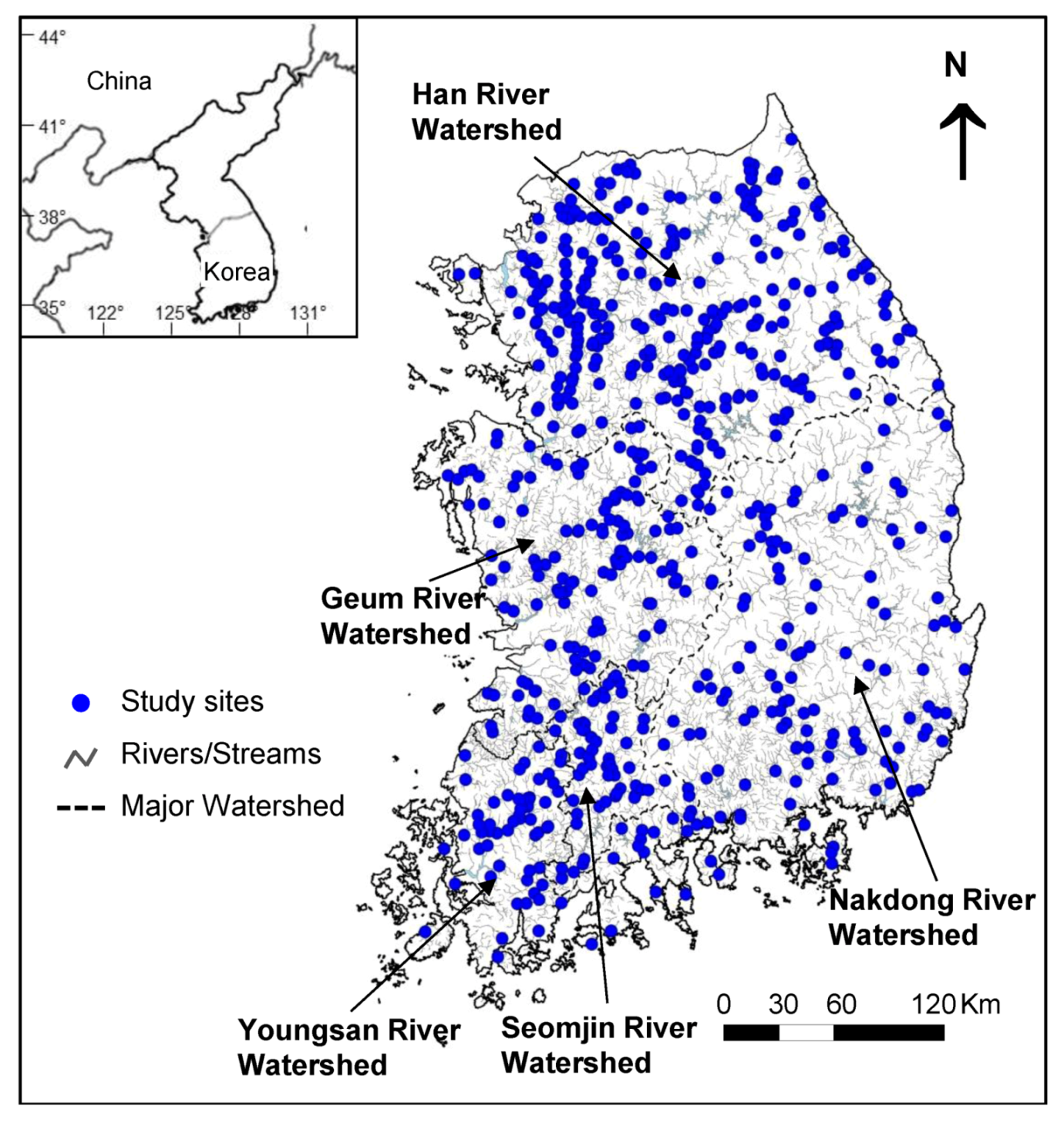
In this study, we evaluated the relationship between fish communities and environmental variables at 691 sampling sites throughout South Korea. Our goals were as follows: (1) to characterize the distributional patterns of fish communities on the national scale, (2) to identify the most important environmental factors influencing the distribution and abundance of fish species for different environmental categories across multiple spatial scales, and (3) to clarify the relative influence of regional and local variables on fish community composition in Korean rivers.
4. Discussion
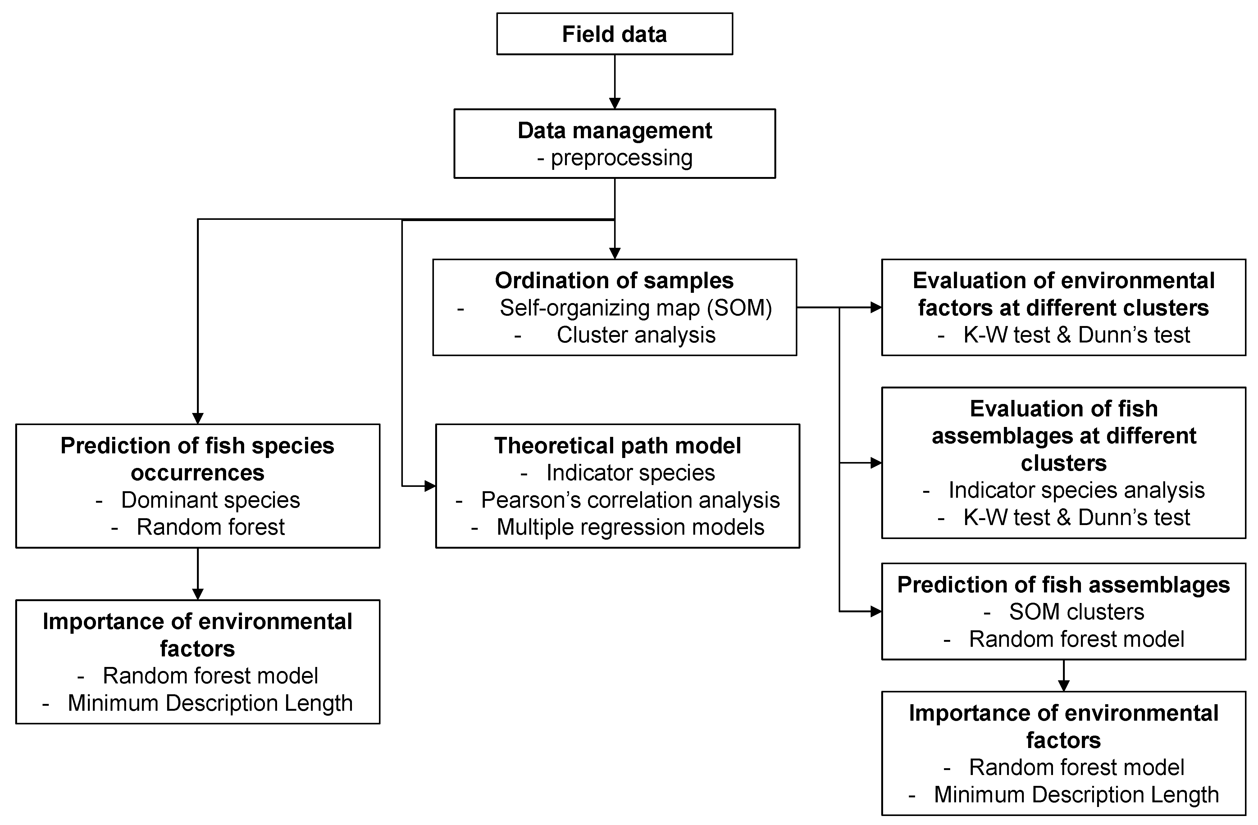
The distribution and abundance of fish communities were characterized with environmental variables across multiple spatial scales using SOM, random forest, and theoretical path models. In this study, we characterized how Korean fish assemblages on a national scale react to changes in the modified longitudinal gradient with various environmental variables at multiple spatial scales, and presented the importance of altitude, DFS, and urban areas for predicting fish community patterns and the occurrence of fish species. These results could provide necessary information for managing fish assemblages and the relationships between changes in fish assemblage and environmental variables.
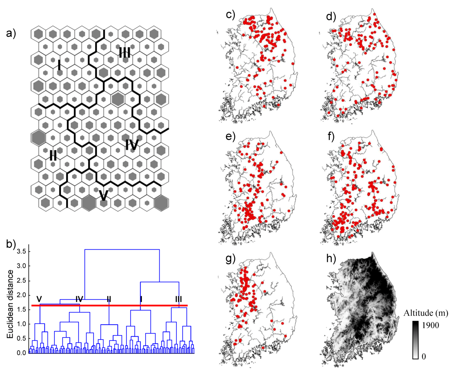
SOM revealed differences among fish communities, reflecting environmental gradients such as the longitudinal gradient from upstream to downstream, and differences in land cover, water quality,
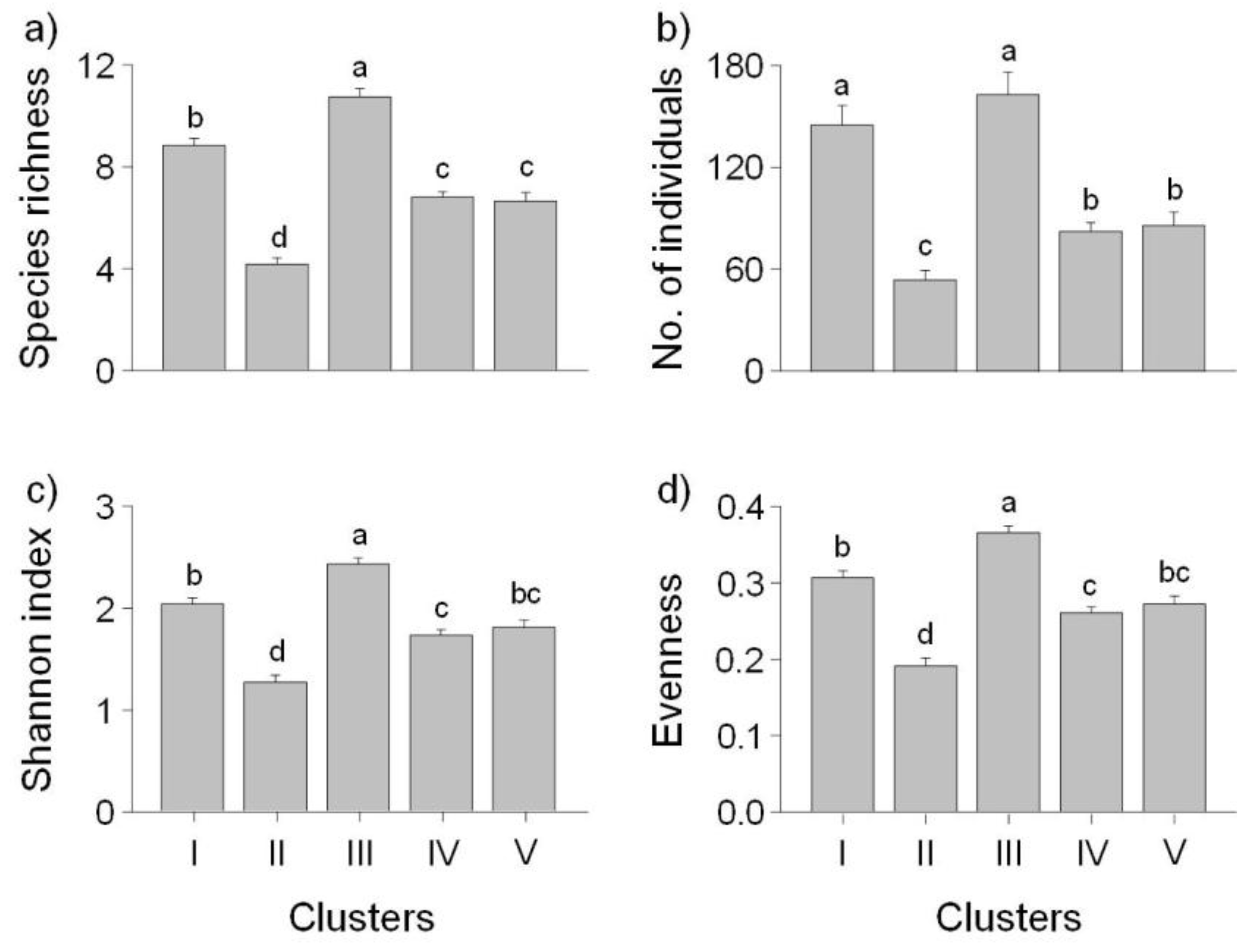
etc. For example, sites in cluster I were from small streams (25.7% of the streams less than third order with high altitude and short DFS), whereas most sites in cluster IV were located further downstream (39.9% of streams were greater than the seventh order with low altitude and long DFS). Species richness and abundance were significantly lower at downstream sites, and high values were found at mid-stream sites. However, previous studies have reported trends where the lowest species richness and abundance is found in headwater streams and the highest levels are downstream at low altitudes [
13,
60,
61,
62,
63]. These studies highlighted the importance of habitat size, because the larger area supported higher species richness and abundance. However, this concept was primarily applied to areas without disturbances. In the current study, the sampling sites showed a wide range of disturbances but general longitudinal gradients of fish species richness were observed after excluding severely polluted sites from the analysis. Oberdorff
et al. [
64] support our findings that species richness reached the maximum in midsize rivers, and then decreased in large rivers. The proportion of forest area decreased downstream, whereas agricultural and urban areas increased, creating an increase in nutrient and pollutant inputs to streams [
65]. The moderate increase of nutrients in the middle stream led to increased species richness, while high nutrients may have reduced the species richness. This supports the intermediate disturbance hypothesis [
66,
67,
68].
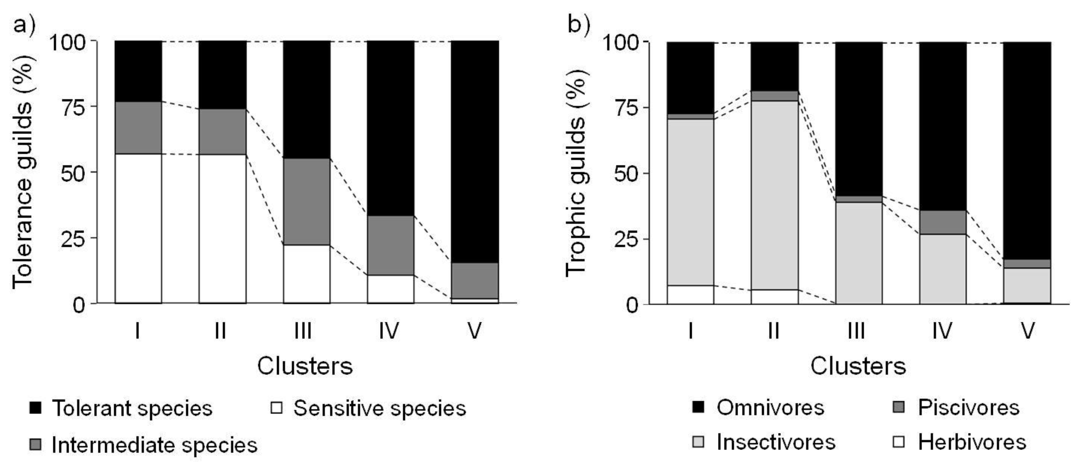
Trophic guilds as well as species richness changed along the upstream-downstream gradient. This result supported the River Continuum Concept [
69]. The proportions of herbivores and insectivores were significantly higher further upstream than downstream, whereas the proportion of omnivores was relatively high downstream (
Figure 5). The trophic composition of the fish communities was induced by the available food resources [
64]. Lowe-McConnell [
70] and Rahel and Hubert [
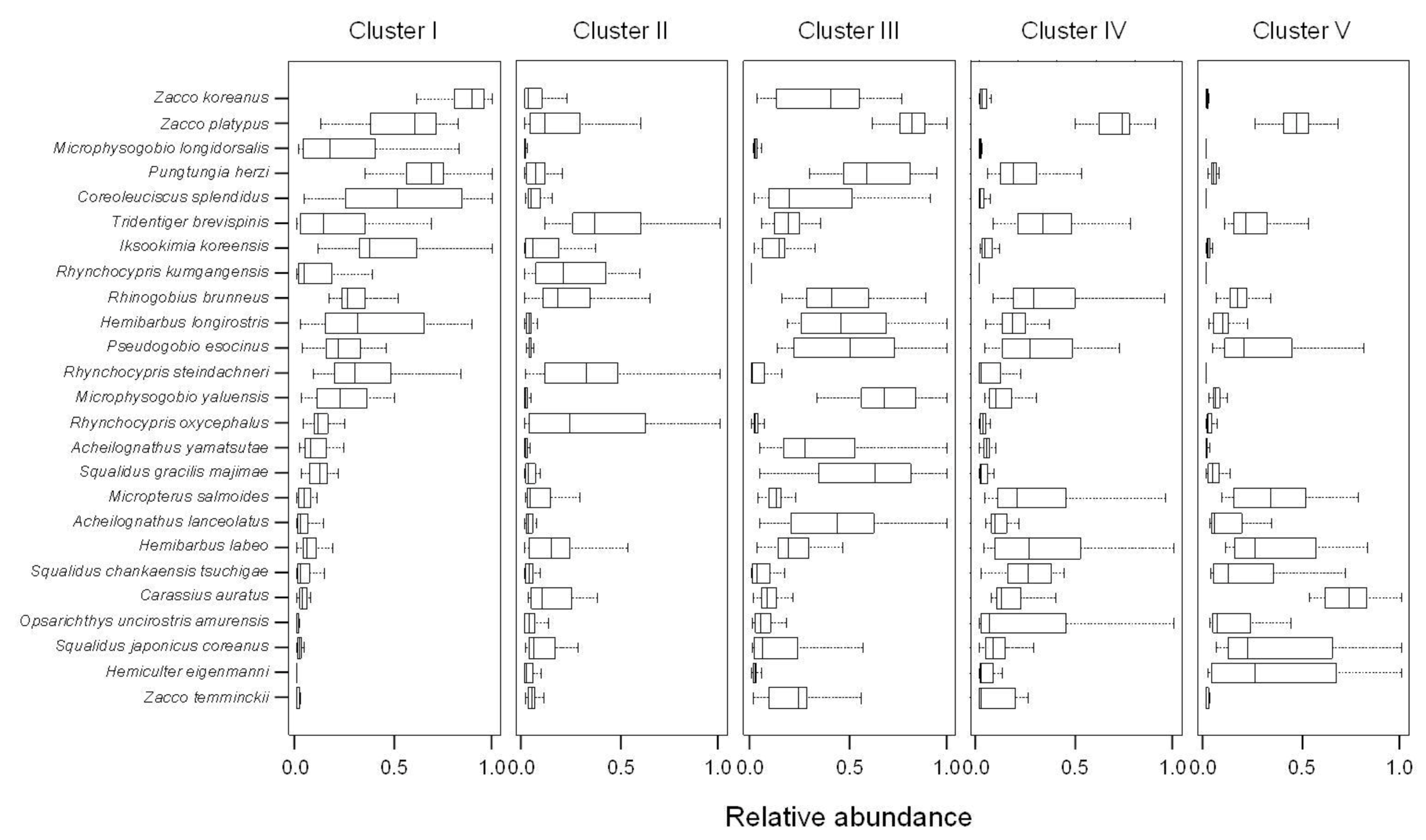
71] reported similar results; headwater streams had higher proportions of insectivorous species, while omnivores were more common in large rivers. These gradients in longitudinal distribution were found at the species level (
Figure 6). Insectivores such as
Iksookimia koreensis,
C. splendidus, and
Z. koreanus were mainly distributed in cluster I, and their relative abundance gradually decrease towards clusters III and IV. Piscivores, such as
O. uncirostris, showed relatively high abundance in cluster IV, and gradually decreased toward cluster I.
Urbanization was correlated with low fish abundance and richness and urban sites were dominated by disturbance-tolerant species [
72]. Urbanization can lead to high concentrations of TP and TN [
73], however, fish diversity and abundances in urban catchments have been found to be dramatically lower than in forested catchments [
74,
75,
76]. This relationship indicates that urbanization can exert a major influence on water quality, habitat, and biological assemblages [
65]. Similarly, agricultural exploitation can also influence aquatic organisms and their environments. Many studies have reported that agricultural activities degrade water quality, affect both riparian and stream habitat quality, and alter water flow [
65]. Fish and macroinvertebrate biodiversity has been documented to decrease with a greater percentage of agricultural land [
77,
78,
79].
Fish assemblages can be influenced by changes in environmental variables such as physical habitat and land use [
80,
81,
82,
83]. Stream gradient, stream order, hydrologic regime, and channel morphology were highly correlated with species richness [
84,
85,
86]. Joy and Death [
87] showed that altitude and distance from the coast were important in a model predicting regional freshwater fish occurrence in the Manawatu–Wanganui region of New Zealand. He
et al. [
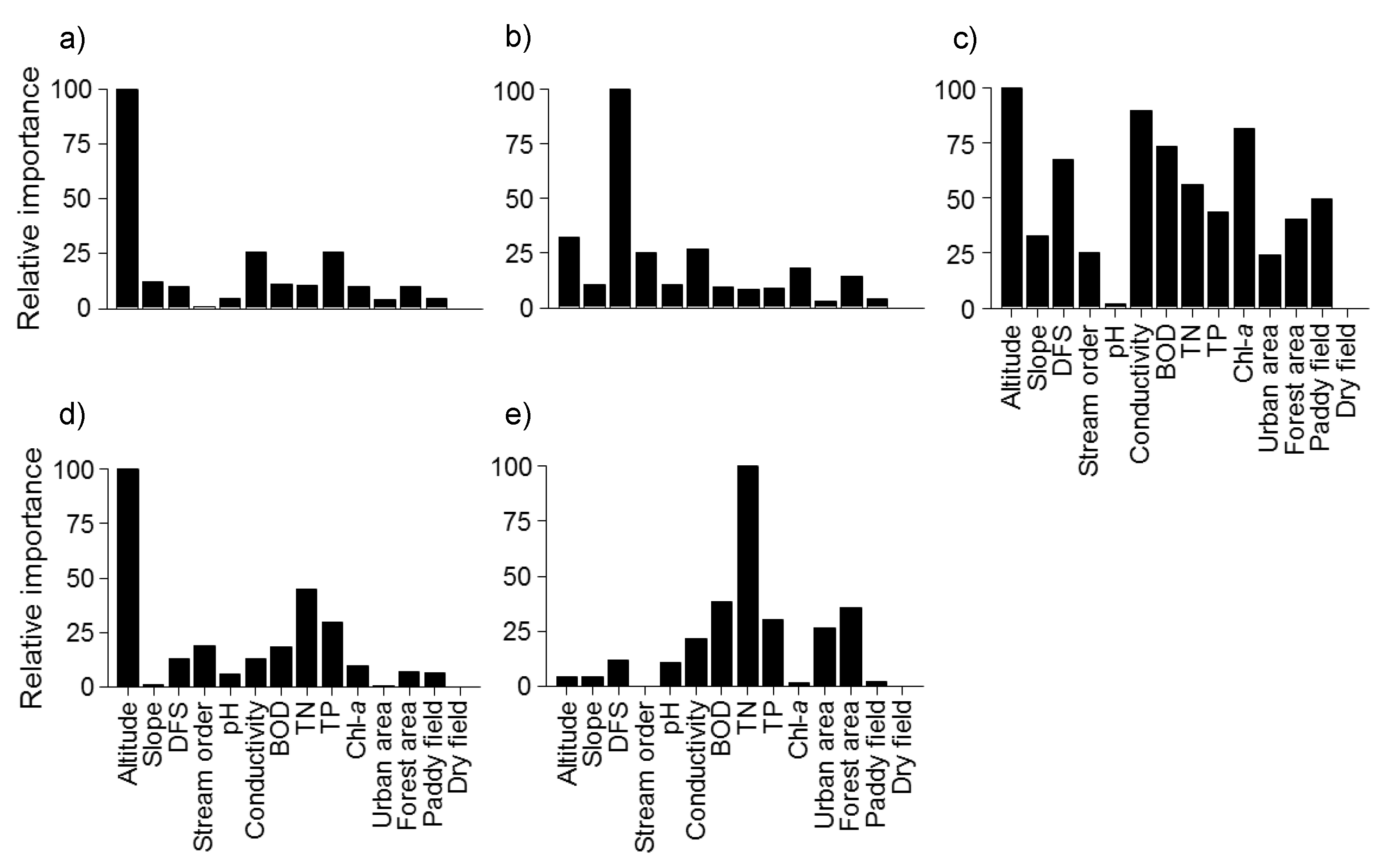
27] also stated that altitude and stream length played important roles in driving the observed endemic fish assemblage structure. Altitude and DFS were also important variables for the prediction of fish community patterns in this study (
Figure 7). Especially, altitude was the most important variable for the prediction of fish community pattern in Clusters I, III and IV, an indication of longitudinal gradients.
Altitude and DFS were the most important factors in 11 of the 15 indicator species. These 11 were indicator species for clusters I and III, which had relatively high altitude.
Coreoperca herzi was an indicator species for cluster I, and DFS and TP were relatively important for predicting the occurrence of
C. herzi. Samples in cluster I were located in upstream locations with a short DFS and a low concentration of TP (
Table 4). Urban land cover was the most important variable for predicting the distribution of
Liobagrus andersoni and
Koreocobitis rotundicaudata, which were indicator species of cluster I. Changes in land use can affect assemblage composition, and lead to changes in the contaminant level of streams [
88]. TN and TP were the most important variables for predicting the distribution of
Cyprinus carpio and
C. auratus, which were indicator species for cluster V.
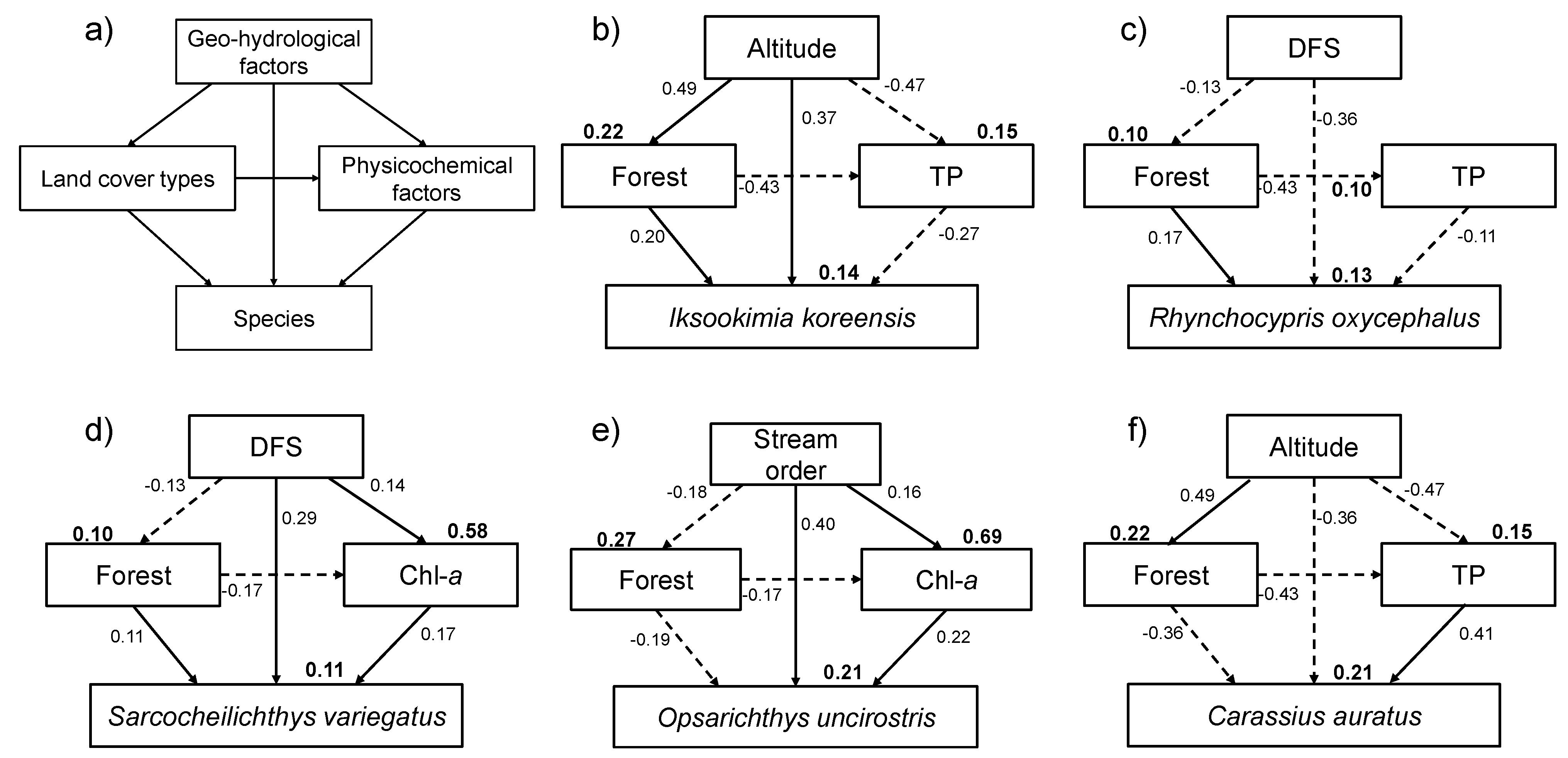
Similarly, the theoretical path model described different responses of species to their environment at multiple spatial scales (
Figure 8). Geographical attributes persist over a relatively long time and influence the development and selection of species’ life history and behavioral traits [
89]; and the surrounding conditions (e.g., slope and stream order) of a stream can also directly and indirectly affect stream habitats [
1,
90]. The theoretical path model showed significant correlations between geo-hydrological factors, land cover types, and physicochemical factors. Among land cover types, forest area displayed the highest correlation with five dominant species, and Chl-
a and TP were the most important physicochemical factors for explaining species occurrences, indicating the importance of water quality in micro-habitat condition. Li
et al. [
1] reported similar results on benthic macro-invertebrates in the same study area. There are many reports of a strong correlation between geographical location and stream communities [
91,
92] and of the importance of altitude [
3,
93].
The random forest model is a non-parametric method for predicting and assessing the relationship between a large number of potential predictor variables and response variables [
47]. Cutler
et al. [
48] reported that the random forest model demonstrated its learning and predicative power as well as its explanatory capacities by presenting a high capability for modeling ecological problems involving non-linear relationships between data. Random forest models have several advantages compared to other statistical methods, such as high classification accuracy, a novel method of determining variable importance, and the ability to model complex interactions among predictor variables [
48]. Therefore, the random forest model offers powerful alternatives to traditional parametric and semiparametric statistical methods for the analysis of ecological data. In addition, He
et al. [
27] showed that mixed models that included both land cover and river characteristic variables were more powerful at explaining the endemic fish distribution patterns in the upper Yangtze River, similar to our results. In our study, the random forest model was more powerful for predicting fish community patterns using all 14 environmental factors than models using either a single variable or another combination of environmental variables (
Table 5).
Many studies have been conducted on the relationships between changes in fish community structure and environmental variables [
71,
82,
83], and most studies have considered some environmental variables such as physical habitat and land use at the local or watershed scale [
94]. Although the distribution and abundance of species are closely linked to small-scale habitat availability [
95], they are also influenced by variables at larger spatial scales [
91]. Regional variables may operate as “filters” constraining species at lower scales through selective habitat forces [
22]. Consequently, preservation and conservation strategies for maintaining stream integrity will be more effective if they are treated as a part of landscape development rather than an isolated entity [
1]. Future studies to benefit conservation and management may consider the influences of global processes on biodiversity, the interactions between these three spatial scales, and the effects of global warming on fish communities.

 ,
, 


 25-75% percentiles,
  non-outlier range).


