
On the Power and Size Properties of Cointegration Tests in the Light of High-Frequency Stylized Facts

Abstract
:1. Introduction
- In a basic approach, an AR(1) and an AR(1)-GARCH(1,1) model are chosen, representing one stationary (or nonstationary) regime with arbitrage permanently occurring.
- A sophistication is given by a MR(3)-STAR(1)1-GARCH(1,1) with its different regimes to model the impact of transaction cost on arbitrage: In its middle regime, the cointegration residual truly behaves like a random walk; in this domain, arbitrage is not yet profitable. However, once the cointegration residual ventures into the outer regimes, arbitrage starts to occur.
- An alternative addition of non-reversible jumps represents idiosyncratic information, affecting only one of the two companies. Such a jump translates into a regime shift, causing further arbitrage to occur, but at a different level. A similar motivation is given in [25], who define “permanent” or “innovation jumps” as regime shifts in the fundamental value of a firm.
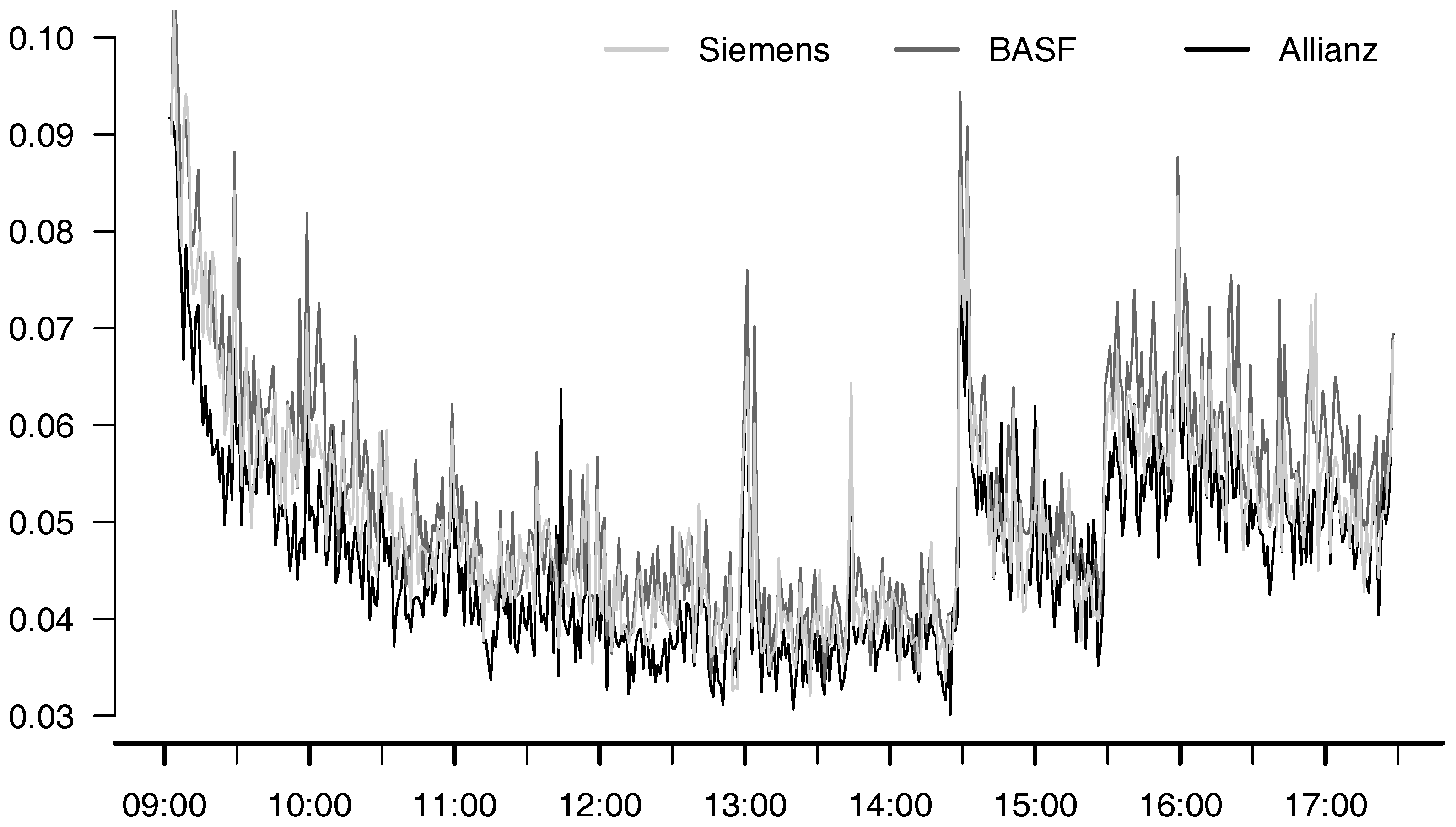
2. Data Sample and Its Stylized Facts
3. Methodology
3.1. Simulation of Stock Prices
- Set the return index i equal to one for initiation, i.e., to the first return of the day. Initialize a vector v with length 509 with zeros.
- Draw one stock s out of the 30 DAX 30 constituents.
- Draw one day d out of 249 full trading days.
- Draw a random block length l from a geometric distribution with expected value of four 2.
- Choose a block of length l, consisting of returns from stock s from day d for indices . Copy these returns in vector v at positions .
- Update i with . Go back to Step 1, until vector v consists of 509 returns.
- Draw a random starting price between 5 and 40 from a uniform distribution. Accumulate the return vector v to a price series.
3.2. Simulation of Cointegration Residuals
3.2.1. Autoregressive Model
3.2.2. Generalized Autoregressive Conditional Heteroscedasticity Model
3.2.3. Multiple Regime Smooth Transition Autoregressive Model
3.2.4. Multiple Regime Smooth Transition Autoregressive Model with Reversible Jumps
3.2.5. Multiple Regime Smooth Transition Autoregressive Model with Non-reversible Jumps
3.2.6. Parameter Choices Common to All Monte Carlo Variants
3.3. The Cointegration Relationship
3.4. Study Design
3.4.1. Cointegration Tests
3.4.2. Setup of Monte Carlo Simulations
4. Results
4.1. Results Type I through Type III
4.2. Results Type IV
4.3. Results Type V
4.4. Results Type VI
5. Conclusions
Acknowledgments
Author Contributions
Conflicts of Interest
References
- E. Elyasiani, and A.E. Kocagil. “Interdependence and dynamics in currency futures markets: A multivariate analysis of intraday data.” J. Bank. Financ. 25 (2001): 1161–1186. [Google Scholar] [CrossRef]
- J. Hasbrouck. “Intraday price formation in U.S. equity index markets.” J. Finance 58 (2003): 2375–2399. [Google Scholar] [CrossRef]
- C.L. Dunis, G. Giorgioni, J. Laws, and J. Rudy. Statistical Arbitrage and High-Frequency Data with an Application to Eurostoxx 50 Equities. Working Paper; Liverpool, UK: Liverpool Business School, 2010. [Google Scholar]
- P.C. Pati, and P. Rajib. “Intraday return dynamics and volatility spillovers between NSE S&P CNX Nifty stock index and stock index futures.” Appl. Econ. Lett. 18 (2011): 567–574. [Google Scholar]
- J. Yang, Z. Yang, and Y. Zhou. “Intraday price discovery and volatility transmission in stock index and stock index futures markets: Evidence from China.” J. Futur. Mark. 32 (2012): 99–121. [Google Scholar] [CrossRef]
- S. Johansen. “Statistical analysis of cointegration vectors.” J. Econ. Dyn. Control 12 (1988): 231–254. [Google Scholar] [CrossRef]
- S. Johansen, and K. Juselius. “Maximum likelihood estimation and inference on cointegration–With applications to the demand for money.” Oxf. Bull. Econ. Stat. 52 (1990): 169–210. [Google Scholar] [CrossRef]
- S. Johansen. “Estimation and hypothesis testing of cointegration vectors in Gaussian vector autoregressive models.” Econometrica 59 (1991): 1551–1580. [Google Scholar] [CrossRef]
- J.J. Kremers, N.R. Ericsson, and J.J. Dolado. “The power of cointegration tests.” Oxf. Bull. Econ. Stat. 54 (1992): 325–348. [Google Scholar] [CrossRef]
- A.A. Haug. “Tests for cointegration a Monte Carlo comparison.” J. Econom. 71 (1996): 89–115. [Google Scholar] [CrossRef]
- K. Hubrich, H. Lütkepohl, and P. Saikkonen. “A review of systems cointegration tests.” Econom. Rev. 20 (2001): 247–318. [Google Scholar] [CrossRef]
- H.P. Boswijk, A. Lucas, and N. Taylor. A Comparison of Parametric, Semi-Nonparametric, Adaptive, and Nonparametric Cointegration Tests. Amsterdam, The Netherlands: Tinbergen Institute Discussion Papers, 1999. [Google Scholar]
- A. Rahbek, E. Hansen, and J.G. Dennis. ARCH Innovations and Their Impact on Cointegration Rank Testing. Working Paper; Copenhagen, Denmark: Department of Theoretical Statistics, University of Copenhagen, 2002. [Google Scholar]
- G. Cavaliere, A. Rahbek, and A.M.R. Taylor. “Testing for co-integration in vector autoregressions with non-stationary volatility.” J. Econom. 158 (2010): 7–24. [Google Scholar] [CrossRef]
- G. Cavaliere, A. Rahbek, and A.M.R. Taylor. “Cointegration rank testing under conditional heteroskedasticity.” Econometr. Theor. 26 (2010): 1719–1760. [Google Scholar] [CrossRef]
- N.S. Balke, and T.B. Fomby. “Threshold cointegration.” Int. Econ. Rev. 38 (1997): 627–645. [Google Scholar] [CrossRef]
- B.E. Hansen, and B. Seo. “Testing for two-regime threshold cointegration in vector error-correction models.” J. Econom. 110 (2002): 293–318. [Google Scholar] [CrossRef]
- M. Seo. “Bootstrap testing for the null of no cointegration in a threshold vector error correction model.” J. Econom. 134 (2006): 129–150. [Google Scholar] [CrossRef]
- C. Alexander. “Optimal hedging using cointegration.” Philos. Trans. R. Soc. Lond. A Math. Phys. Eng. Sci. 357 (1999): 2039–2058. [Google Scholar] [CrossRef]
- C. Alexander, and A. Dimitriu. “Indexing and statistical arbitrage.” J. Portf. Manag. 31 (2005): 50–63. [Google Scholar] [CrossRef]
- E. Gatev, W.N. Goetzmann, and K.G. Rouwenhorst. “Pairs trading: Performance of a relative-value arbitrage rule.” Rev. Financial Stud. 19 (2006): 797–827. [Google Scholar] [CrossRef]
- J.E. Ingersoll. Theory of Financial Decision Making. Totowa, NJ, USA: Rowman & Littlefield, 1987. [Google Scholar]
- Z. Chen, and P.J. Knez. “Measurement of market integration and arbitrage.” Rev. Financial Stud. 8 (1995): 287–325. [Google Scholar] [CrossRef]
- S. Andrade, V. Di Pietro, and M. Seasholes. Understanding the Profitability of Pairs Trading. Working Paper; Evanston, IL, USA: UC Berkeley, Northwestern University, 2005. [Google Scholar]
- E. Jondeau, J. Lahaye, and M. Rockinger. “Asymmetry in the price impact of trades in an high-frequency microstructure model with jumps.” J. Bank. Finance. 61 (2015): 205–224. [Google Scholar] [CrossRef]
- A. Trapletti, K. Hornik, and B. LeBaron. “tseries: Time series analysis and computational finance.” Available online: https://cran.r-project.org/web/packages/tseries/index.html (accessed on 6 February 2017).
- R Development Core Team. “R: A language and environment for statistical computing.” Available online: https://www.r-project.org/ (accessed on 6 February 2017).
- S. Graves. “FinTS: Companion to Tsay (2005) Analysis of financial time series.” Available online: https://rdrr.io/cran/FinTS/ (accessed on 6 February 2017).
- O.E. Barndorff-Nielsen, and N. Shephard. “Econometrics of testing for jumps in financial economics using bipower variation.” J. Financial Econom. 4 (2006): 1–30. [Google Scholar] [CrossRef]
- K. Boudt, J. Cornelissen, S. Payseur, G. Nguyen, and M. Schermer. “High frequency: Tools for high frequency data analysis.” Available online: https://rdrr.io/cran/highfrequency/ (accessed on 6 February 2017).
- K.S. Chan, and B. Ripley. “TSA: Time series analysis.” Available online: https://rdrr.io/cran/TSA/ (accessed on 6 February 2017).
- R. Luukkonen, P. Saikkonen, and T. Teräsvirta. “Testing linearity against smooth transition autoregressive models.” Biometrika 75 (1988): 491–499. [Google Scholar] [CrossRef]
- A. Ghalanos. “Twinkle: Dynamic smooth transition ARMAX models.” Available online: http://past.rinfinance.com/agenda/2014/talk/AlexiosGhalanos.pdf (accessed on 6 February 2017).
- A. Ghalanos. “Rugarch: Univariate GARCH models.” Available online: https://rdrr.io/cran/rugarch/ (accessed on 6 February 2017).
- R.F. Engle, and M.E. Sokalska. “Forecasting intraday volatility in the US equity market: Multiplicative component GARCH.” J. Financial Econom. 10 (2012): 54–83. [Google Scholar] [CrossRef]
- K. Herrmann, S. Teis, and W. Yu. Components of Intraday Volatility and Their Prediction at Different Sampling Frequencies with Application to DAX and BUND Futures. IWQW Discussion Paper Series; Erlangen, Germany: University of Erlangen-Nürnberg, 2014. [Google Scholar]
- R. Cont. “Empirical properties of asset returns: Stylized facts and statistical issues.” Quantit. Finance 1 (2001): 223–236. [Google Scholar] [CrossRef]
- B. Pfaff. Analysis of Integrated and Cointegrated Time Series with R. New York, NY, USA: Springer, 2008. [Google Scholar]
- D.A. Dickey, and W.A. Fuller. “Distribution of the estimators for autoregressive time series with a unit root.” J. Am. Stat. Assoc. 74 (1979): 427–431. [Google Scholar] [CrossRef]
- R.S. Tsay. Multivariate Time Series Analysis: With R and Financial Applications. Wiley Series in Probability and Statistics; Hoboken, NJ, USA: John Wiley & Sons, 2014. [Google Scholar]
- J.A. Doornik. “Approximations to the asymptotic distributions of cointegration tests.” J. Econ. Surv. 12 (1998): 573–593. [Google Scholar] [CrossRef]
- F. Yang. “CommonTrend: Extract and plot common trends from a cointegration system. Calculate p-value for Johansen statistics. ” Available online: https://rdrr.io/cran/CommonTrend/ (accessed on 6 February 2017).
- B.M. Hill. “A simple general approach to inference about the tail of a distribution.” Ann. Statist. 3 (1975): 1163–1174. [Google Scholar] [CrossRef]
- J. Breitung. “Rank tests for nonlinear cointegration.” J. Bus. Econ. Stat. 19 (2001): 331–340. [Google Scholar] [CrossRef]
- M. Clegg. “On the persistence of cointegration in pairs trading. ” Available online: https://ssrn.com/abstract=2491201 (accessed on 6 February 2017).
- D.N. Politis, and J.P. Romano. “The stationary bootstrap.” J. Am. Stat. Assoc. 89 (1994): 1303–1313. [Google Scholar] [CrossRef]
- A. Azzalini, and A. Capitanio. The Skew-Normal and Related Families. Cambridge, UK: Cambridge University Press, 2014. [Google Scholar]
- G. Hong, and R. Susmel. Pairs-Trading in the Asian ADR Market. Working Paper; Houston, TX, USA: University of Houston, 2003. [Google Scholar]
- T. Bollerslev. “Generalized autoregressive conditional heteroskedasticity.” J. Econom. 31 (1986): 307–327. [Google Scholar] [CrossRef]
- D.B. Nelson. “Stationarity and persistence in the GARCH(1,1) model.” Econometr. Theor. 6 (1990): 318–334. [Google Scholar] [CrossRef]
- L.R. Glosten, R. Jagannathan, and D.E. Runkle. “On the relation between the expected value and the volatility of the nominal excess return on stocks.” J. Finance 48 (1993): 1779–1801. [Google Scholar] [CrossRef]
- D.B. Nelson. “Conditional heteroskedasticity in asset returns: A new approach.” Econometrica 59 (1991): 347–370. [Google Scholar] [CrossRef]
- M. McAleer, F. Chan, S. Hoti, and O. Lieberman. “Generalized autoregressive conditional correlation.” Econometr. Theor. 24 (2008): 1554–1583. [Google Scholar] [CrossRef]
- H. Tong. “On a threshold model.” In Pattern Recognition and Signal Processing. Nato Advanced Study Institutes: Series E, Applied Sciences; Edited by C.H. Chen. Alphen aan den Rijn, The Netherlands: Sijthoff & Noordhoff, 1978, Volume 29. [Google Scholar]
- T. Teräsvirta. “Specification, estimation, and evaluation of smooth transition autoregressive models.” J. Am. Stat. Assoc. 89 (1994): 208–218. [Google Scholar] [CrossRef]
- D. van Dijk, and P.H. Franses. “Modeling multiple regimes in the business cycle.” Macroecon. Dyn. 3 (1999): 311–340. [Google Scholar] [CrossRef]
- F. Chan, and M. McAleer. “Maximum likelihood estimation of STAR and STAR-GARCH models: Theory and Monte Carlo evidence.” J. Appl. Econom. 17 (2002): 509–534. [Google Scholar] [CrossRef]
- F. Chan, and M. McAleer. “Estimating smooth transition autoregressive models with GARCH Errors in the presence of extreme observations and outliers.” Appl. Financial Econ. 13 (2003): 581–592. [Google Scholar] [CrossRef]
- K.S. Chan, J.D. Petruccelli, H. Tong, and S.W. Woolford. “A multiple-threshold AR(1) model.” J. Appl. Probab. 22 (1985): 267. [Google Scholar] [CrossRef]
- S.M. Ross. Stochastic Processes, 2nd ed. Wiley Series in Probability and Statistics; Probability and Statistics; New York, NY, USA: Wiley, 1996. [Google Scholar]
- B.W. Silverman. Density Estimation for Statistics and Data Analysis. London, UK: New York, NY, USA: Chapman and Hall, 1986. [Google Scholar]
- S.J. Sheather, and M.C. Jones. “A reliable data-based bandwidth selection method for kernel density estimation.” J. R. Stat. Soc. Ser. B, 1991, 683–690. [Google Scholar]
- D.A. Dickey, and W.A. Fuller. “Likelihood ratio statistics for autoregressive time series with a unit root.” Econometrica 49 (1981): 1057–1072. [Google Scholar] [CrossRef]
- P. Perron. “Trends and random walks in macroeconomic time series.” J. Econ. Dyn. Control 12 (1988): 297–332. [Google Scholar] [CrossRef]
- P.C.B. Phillips, and S. Ouliaris. “Asymptotic properties of residual based tests for cointegration.” Econometrica 58 (1990): 165–193. [Google Scholar] [CrossRef]
- S.G. Pantula, G. Gonzalez-Farias, and W.A. Fuller. “A comparison of unit-root test criteria.” J. Bus. Econ. Stat. 12 (1994): 449–459. [Google Scholar] [CrossRef]
- J. Breitung. “Nonparametric tests for unit roots and cointegration.” J. Econom. 108 (2002): 343–363. [Google Scholar] [CrossRef]
- J. Breitung, and A.M.R. Taylor. “Corrigendum to “Nonparametric tests for unit roots and cointegration” [J. Econom. 108 (2002) 343–363].” J. Econom. 117 (2003): 401–404. [Google Scholar] [CrossRef]
- G. Elliott, T.J. Rothenberg, and J.H. Stock. “Efficient tests for an autoregressive unit root.” Econometrica 64 (1996): 813–836. [Google Scholar] [CrossRef]
- P. Schmidt, and P.C.B. Phillips. “LM tests for a unit root in the presence of deterministic trends.” Oxf. Bull. Econ. Stat. 54 (1992): 257–287. [Google Scholar] [CrossRef]
- G. Cavaliere. “Testing the unit root hypothesis using generalized range statistics.” Econom. J. 4 (2001): 70–88. [Google Scholar] [CrossRef]
- D. Wuertz, and M.S. Taqqu. “fArma: ARMA time series modelling.” Available online: https://rdrr.io/cran/fArma/ (accessed on 6 February 2017).
- C. Krauss. “Statistical arbitrage pairs trading strategies: Review and outlook.” J. Econ. Surv. Forthcom., 2016. [Google Scholar] [CrossRef]
- C. Alexander. Practical Financial Econometrics, Reprinted March 2009 ed. Volume 2—Market Risk Analysis; Chichester, UK: Wiley, 2009. [Google Scholar]
- 1.Multiple regime smooth transition autoregressive process.
- 2.A value of four is chosen ad hoc, as a compromise between partially preserving serial dependence in returns or squared returns and sufficient randomization. The latter refers to the fact that setting large block lengths leads to the risk of creating the simulated time series just on the basis of a few selected stocks. A value of four puts more emphasis on introducing a higher level of diversity.
- 3.We replicate the analyses of Table 1 on bootstrap simulated data in order to see if the bootstrap preserves the stylized facts. It turns out that almost all results are very similar. We mainly observe a decrease in detected ARCH effects, as volatility patterns cannot be perfectly replicated with small block lengths.
- 4.The point at which converges to zero depends on the choice of γ.
- 5.Clearly, the mixed AR coefficient varies with the parameters , but for simplicity reasons and better comparability, it was fixed ad hoc at 0.95.
- 6.This auxiliary metric is used to define fixed thresholds, even in light of potential non-stationarities.
- 7.To see this effect, estimate the AR(1)-coefficient of two processes: (1) a simple stationary AR(1)-process with coefficient ; and (2) the same process contaminated by a single large non-reversible jump. The estimate of the latter is biased towards the nonstationary case.
- 8.For such an estimation, the median of the absolute value of t-distributed innovations with five degrees of freedom and standard deviation of 0.0059 can be calculated as 0.0033. See Table 3 for the relevant parameter values used in this estimation.


| Type | Test | Raw Returns | AR(1) | AR(1)-GARCH(1,1) |
|---|---|---|---|---|
| Non-normality | Jarque–Bera test | 1.00 | 1.00 | 1.00 |
| Box test | 0.57 | 0.55 | 0.03 | |
| ARCH effects | Engle’s ARCH test | 0.71 | 0.69 | 0.04 |
| BDS test | 0.84 | 0.76 | 0.24 | |
| Tsay test | 0.50 | 0.45 | 0.23 | |
| Luukkonen test | 0.41 | 0.40 | 0.08 | |
| Nonlinearity | Teräsvirta test | 0.37 | 0.36 | 0.07 |
| Jumps | BNS test | 1.00 | 0.99 | 1.00 |
| Type | Test | Raw Data | AR(1) | AR(1)-GARCH(1,1) |
|---|---|---|---|---|
| Non-normality | Jarque–Bera test | 0.89 | 0.99 | 0.99 |
| Box test | 1.00 | 0.70 | 0.13 | |
| ARCH effects | Engle’s ARCH test | 1.00 | 0.75 | 0.07 |
| BDS test | 1.00 | 0.64 | 0.49 | |
| Tsay test | 0.45 | 0.54 | 0.27 | |
| Luukkonen test | 0.55 | 0.38 | 0.15 | |
| Nonlinearity | Teräsvirta test | 0.55 | 0.35 | 0.16 |
| Jumps | BNS test | 1.00 | 0.98 | 1.00 |
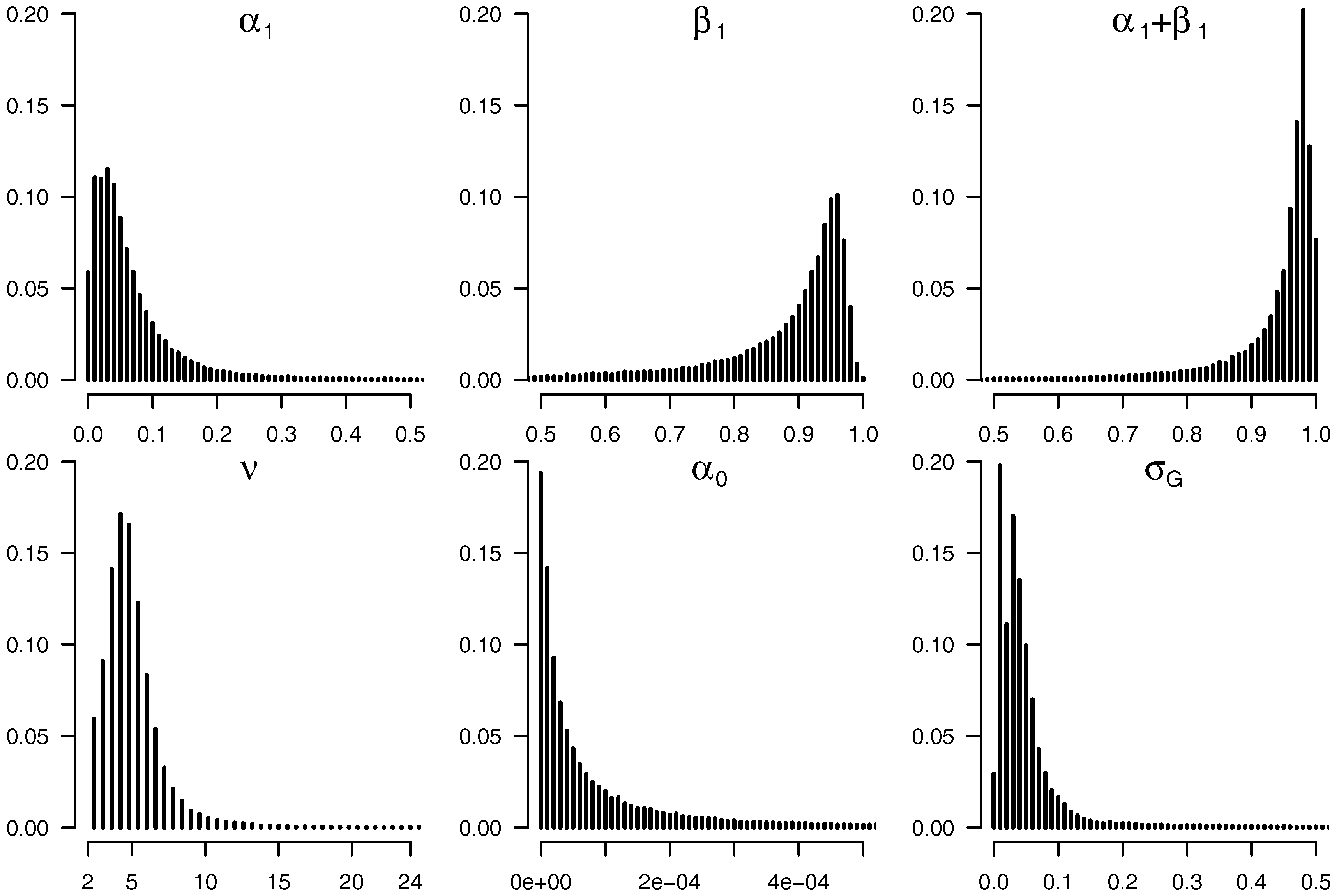
| ν | |||||||
|---|---|---|---|---|---|---|---|
| Minimum | 0.75187 | 0.00000 | 0.00000 | 0.00000 | 0.00000 | 2.10000 | 0.00000 |
| 1st Quartile | 0.95820 | 0.00001 | 0.02244 | 0.84915 | 0.93438 | 3.74772 | 0.00029 |
| Median | 0.97370 | 0.00004 | 0.04491 | 0.92124 | 0.96879 | 4.62810 | 0.00119 |
| Mean | 0.96904 | 0.00016 | 0.06414 | 0.87542 | 0.93956 | 5.05612 | 0.00585 |
| 3rd Quartile | 0.98516 | 0.00012 | 0.08126 | 0.95268 | 0.98277 | 5.69619 | 0.00312 |
| Maximum | 1.00000 | 0.03982 | 0.92903 | 0.99900 | 0.99900 | 99.99361 | 0.27104 |
| Panel A: Number of Jumps per Day | Mean | |||||
| Reversible jumps | 0.00 | 2.00 | 3.00 | 3.66 | 5.00 | 8.00 |
| Non-reversible jumps | 2.00 | 4.00 | 6.00 | 6.88 | 8.00 | 13.00 |
| Panel B: Size of Jumps in EUR | Mean | |||||
| Reversible jumps | 0.02 | 0.05 | 0.10 | 0.12 | 0.16 | 0.31 |
| Non-reversible jumps | 0.02 | 0.06 | 0.11 | 0.17 | 0.19 | 0.45 |
| Cointegration Test | R Implementation | ||
|---|---|---|---|
| Augmented Dickey–Fuller test | [39,63] | tseries | [26] |
| Phillips–Perron test | [64,65] | tseries | [26] |
| Pantula, Gonzalez-Farias and Fuller test | [66] | egcm | [45] |
| Breitung’s variance ratio test | [67,68] | egcm | [45] |
| Johansen’s eigenvalue test | [6,7,8] | urca, vars | [38] |
| Johansen’s trace test | [6,7,8] | urca, vars | [38] |
| Elliott-Rothenberg-Stock point optimal test | [69] | urca | [38] |
| Elliott-Rothenberg-Stock Dickey-Fuller Generalized Least Squares test | [69] | urca | [38] |
| Schmidt and Phillips rho statistic | [70] | urca | [38] |
| Based on Hurst exponent | [71] | fArma | [72] |
| MC Type | Type I | Type II | Type III | |||||||||
| Process | AR(1) | AR(1) | AR(1)-GARCH(1,1) | |||||||||
| Distribution | Normal | t | t | |||||||||
| 1.00 | 0.95 | 0.90 | 0.85 | 1.00 | 0.95 | 0.90 | 0.85 | 1.00 | 0.95 | 0.90 | 0.85 | |
| MC Type | Type IV | Type V | Type VI | |||||||||
| Process | STAR(1)-GARCH(1,1) | STAR(1)-GARCH(1,1) | STAR(1)-GARCH(1,1) | |||||||||
| Regimes | 3 | 3 | 3 | |||||||||
| Jumps | - | reversible | non-reversible | |||||||||
| Distribution | t | t | t | |||||||||
| 1.00 | 0.95 | 0.90 | 0.85 | 1.00 | 0.95 | 0.90 | 0.85 | 1.00 | 0.95 | 0.90 | 0.85 | |
| 1.00 | 1.00 | 1.00 | 1.00 | 1.00 | 1.00 | 1.00 | 1.00 | 1.00 | 1.00 | 1.00 | 1.00 | |
| 1.00 | 0.95 | 0.90 | 0.85 | 1.00 | 0.95 | 0.90 | 0.85 | 1.00 | 0.95 | 0.90 | 0.85 | |
| –1.00 | –5.00 | –10.00 | –1.00 | –1.00 | ||||||||
| 1.00 | 5.00 | 10.00 | 1.00 | 1.00 | ||||||||
| 1.00 | 5.00 | 10.00 | 5.00 | 5.00 | ||||||||
| 1.00 | 5.00 | 10.00 | 5.00 | 5.00 | ||||||||
| 2.00 | 3.00 | 8.00 | ||||||||||
| 0.05 | 0.10 | 0.30 | ||||||||||
| 4.00 | 6.00 | 12.00 | ||||||||||
| 0.05 | 0.10 | 0.45 | ||||||||||
| 0.850 | 0.900 | 0.950 | |
| 0.956 | 0.963 | 0.971 |
| Test | Type I | Type II | Type III | |
|---|---|---|---|---|
| pp | 1.00 | 0.06 | 0.06 | 0.07 |
| adf | 1.00 | 0.05 | 0.05 | 0.06 |
| jo-e | 1.00 | 0.06 | 0.06 | 0.06 |
| jo-t | 1.00 | 0.06 | 0.06 | 0.07 |
| ers-p | 1.00 | 0.05 | 0.05 | 0.06 |
| ers-d | 1.00 | 0.05 | 0.05 | 0.05 |
| sp-r | 1.00 | 0.05 | 0.05 | 0.05 |
| hurst | 1.00 | 0.05 | 0.05 | 0.06 |
| bvr | 1.00 | 0.05 | 0.05 | 0.05 |
| pgff | 1.00 | 0.06 | 0.06 | 0.06 |
| Test | Type I | Type II | Type III | |
|---|---|---|---|---|
| pp | 0.95 | 0.84 | 0.85 | 0.83 |
| pp | 0.90 | 1.00 | 1.00 | 1.00 |
| pp | 0.85 | 1.00 | 1.00 | 1.00 |
| adf | 0.95 | 0.64 | 0.63 | 0.64 |
| adf | 0.90 | 0.98 | 0.98 | 0.98 |
| adf | 0.85 | 1.00 | 1.00 | 1.00 |
| jo-e | 0.95 | 0.56 | 0.56 | 0.58 |
| jo-e | 0.90 | 1.00 | 1.00 | 0.99 |
| jo-e | 0.85 | 1.00 | 1.00 | 1.00 |
| jo-t | 0.95 | 0.52 | 0.53 | 0.54 |
| jo-t | 0.90 | 0.99 | 0.99 | 0.98 |
| jo-t | 0.85 | 1.00 | 1.00 | 1.00 |
| ers-p | 0.95 | 0.69 | 0.70 | 0.70 |
| ers-p | 0.90 | 0.91 | 0.91 | 0.90 |
| ers-p | 0.85 | 0.97 | 0.96 | 0.96 |
| ers-d | 0.95 | 0.65 | 0.67 | 0.68 |
| ers-d | 0.90 | 0.86 | 0.86 | 0.87 |
| ers-d | 0.85 | 0.92 | 0.92 | 0.92 |
| sp-r | 0.95 | 0.63 | 0.62 | 0.62 |
| sp-r | 0.90 | 0.97 | 0.97 | 0.96 |
| sp-r | 0.85 | 1.00 | 1.00 | 0.99 |
| hurst | 0.95 | 0.43 | 0.44 | 0.44 |
| hurst | 0.90 | 0.73 | 0.72 | 0.73 |
| hurst | 0.85 | 0.84 | 0.85 | 0.85 |
| bvr | 0.95 | 0.53 | 0.53 | 0.54 |
| bvr | 0.90 | 0.81 | 0.81 | 0.81 |
| bvr | 0.85 | 0.91 | 0.91 | 0.91 |
| pgff | 0.95 | 0.87 | 0.89 | 0.87 |
| pgff | 0.90 | 1.00 | 1.00 | 1.00 |
| pgff | 0.85 | 1.00 | 1.00 | 1.00 |
| 1.00 | 1.00 | 1.00 | 5.00 | 5.00 | 5.00 | 10.00 | 10.00 | 10.00 | |||
| Test | 1.00 | 5.00 | 10.00 | 1.00 | 5.00 | 10.00 | 1.00 | 5.00 | 10.00 | ||
| pp | 1.00 | 0.07 | 0.06 | 0.06 | 0.06 | 0.06 | 0.06 | 0.07 | 0.06 | 0.07 | |
| adf | 1.00 | 0.06 | 0.06 | 0.06 | 0.06 | 0.06 | 0.06 | 0.06 | 0.06 | 0.06 | |
| jo-e | 1.00 | 0.07 | 0.07 | 0.07 | 0.07 | 0.07 | 0.07 | 0.07 | 0.07 | 0.07 | |
| jo-t | 1.00 | 0.07 | 0.06 | 0.06 | 0.07 | 0.06 | 0.06 | 0.06 | 0.07 | 0.06 | |
| ers-p | 1.00 | 0.05 | 0.05 | 0.05 | 0.05 | 0.06 | 0.05 | 0.05 | 0.05 | 0.06 | |
| ers-d | 1.00 | 0.05 | 0.05 | 0.05 | 0.05 | 0.05 | 0.05 | 0.05 | 0.06 | 0.05 | |
| sp-r | 1.00 | 0.06 | 0.05 | 0.05 | 0.05 | 0.06 | 0.05 | 0.05 | 0.05 | 0.05 | |
| hurst | 1.00 | 0.05 | 0.05 | 0.05 | 0.05 | 0.05 | 0.05 | 0.06 | 0.05 | 0.05 | |
| bvr | 1.00 | 0.05 | 0.05 | 0.05 | 0.05 | 0.05 | 0.05 | 0.05 | 0.05 | 0.05 | |
| pgff | 1.00 | 0.06 | 0.06 | 0.07 | 0.07 | 0.07 | 0.07 | 0.07 | 0.06 | 0.07 |
| 1.00 | 1.00 | 1.00 | 5.00 | 5.00 | 5.00 | 10.00 | 10.00 | 10.00 | |||
| Test | 1.00 | 5.00 | 10.00 | 1.00 | 5.00 | 10.00 | 1.00 | 5.00 | 10.00 | ||
| pp | 0.95 | 0.78 | 0.65 | 0.59 | 0.54 | 0.23 | 0.16 | 0.38 | 0.13 | 0.10 | |
| pp | 0.90 | 0.99 | 0.97 | 0.95 | 0.90 | 0.41 | 0.27 | 0.70 | 0.22 | 0.13 | |
| pp | 0.85 | 1.00 | 0.98 | 0.97 | 0.95 | 0.51 | 0.34 | 0.81 | 0.28 | 0.16 | |
| adf | 0.95 | 0.58 | 0.46 | 0.42 | 0.39 | 0.17 | 0.13 | 0.28 | 0.11 | 0.09 | |
| adf | 0.90 | 0.96 | 0.87 | 0.81 | 0.80 | 0.33 | 0.20 | 0.58 | 0.18 | 0.11 | |
| adf | 0.85 | 1.00 | 0.95 | 0.93 | 0.92 | 0.43 | 0.27 | 0.74 | 0.23 | 0.13 | |
| jo-e | 0.95 | 0.50 | 0.38 | 0.34 | 0.33 | 0.13 | 0.11 | 0.22 | 0.09 | 0.08 | |
| jo-e | 0.90 | 0.97 | 0.89 | 0.84 | 0.80 | 0.30 | 0.18 | 0.55 | 0.16 | 0.10 | |
| jo-e | 0.85 | 1.00 | 0.97 | 0.95 | 0.92 | 0.40 | 0.25 | 0.74 | 0.22 | 0.11 | |
| jo-t | 0.95 | 0.48 | 0.36 | 0.32 | 0.31 | 0.13 | 0.10 | 0.21 | 0.09 | 0.08 | |
| jo-t | 0.90 | 0.96 | 0.85 | 0.79 | 0.76 | 0.28 | 0.18 | 0.52 | 0.15 | 0.09 | |
| jo-t | 0.85 | 0.99 | 0.96 | 0.94 | 0.90 | 0.38 | 0.23 | 0.71 | 0.20 | 0.11 | |
| ers-p | 0.95 | 0.67 | 0.58 | 0.55 | 0.52 | 0.24 | 0.17 | 0.36 | 0.13 | 0.10 | |
| ers-p | 0.90 | 0.88 | 0.82 | 0.79 | 0.78 | 0.39 | 0.26 | 0.61 | 0.21 | 0.13 | |
| ers-p | 0.85 | 0.95 | 0.91 | 0.88 | 0.87 | 0.47 | 0.31 | 0.73 | 0.25 | 0.16 | |
| ers-d | 0.95 | 0.65 | 0.57 | 0.53 | 0.50 | 0.23 | 0.16 | 0.35 | 0.13 | 0.09 | |
| ers-d | 0.90 | 0.86 | 0.79 | 0.75 | 0.74 | 0.36 | 0.24 | 0.60 | 0.20 | 0.13 | |
| ers-d | 0.85 | 0.92 | 0.86 | 0.83 | 0.84 | 0.46 | 0.30 | 0.70 | 0.25 | 0.14 | |
| sp-r | 0.95 | 0.57 | 0.47 | 0.43 | 0.41 | 0.18 | 0.13 | 0.28 | 0.10 | 0.08 | |
| sp-r | 0.90 | 0.94 | 0.85 | 0.78 | 0.78 | 0.32 | 0.20 | 0.57 | 0.18 | 0.11 | |
| sp-r | 0.85 | 0.99 | 0.95 | 0.91 | 0.90 | 0.41 | 0.26 | 0.72 | 0.21 | 0.13 | |
| hurst | 0.95 | 0.41 | 0.34 | 0.32 | 0.31 | 0.14 | 0.11 | 0.22 | 0.09 | 0.08 | |
| hurst | 0.90 | 0.69 | 0.61 | 0.55 | 0.56 | 0.25 | 0.17 | 0.42 | 0.15 | 0.09 | |
| hurst | 0.85 | 0.83 | 0.74 | 0.69 | 0.71 | 0.32 | 0.22 | 0.55 | 0.19 | 0.11 | |
| bvr | 0.95 | 0.51 | 0.43 | 0.41 | 0.39 | 0.19 | 0.14 | 0.29 | 0.12 | 0.08 | |
| bvr | 0.90 | 0.77 | 0.70 | 0.63 | 0.65 | 0.31 | 0.20 | 0.49 | 0.17 | 0.11 | |
| bvr | 0.85 | 0.90 | 0.81 | 0.76 | 0.78 | 0.38 | 0.25 | 0.63 | 0.22 | 0.12 | |
| pgff | 0.95 | 0.81 | 0.68 | 0.64 | 0.58 | 0.23 | 0.17 | 0.39 | 0.14 | 0.10 | |
| pgff | 0.90 | 1.00 | 0.97 | 0.96 | 0.91 | 0.42 | 0.28 | 0.71 | 0.23 | 0.14 | |
| pgff | 0.85 | 1.00 | 0.98 | 0.97 | 0.95 | 0.52 | 0.35 | 0.82 | 0.28 | 0.17 |
| 2.00 | 2.00 | 2.00 | 3.00 | 3.00 | 3.00 | 8.00 | 8.00 | 8.00 | |||
| Test | 0.05 | 0.10 | 0.30 | 0.05 | 0.10 | 0.30 | 0.05 | 0.10 | 0.30 | ||
| pp | 1.00 | 0.06 | 0.06 | 0.06 | 0.06 | 0.06 | 0.06 | 0.07 | 0.06 | 0.05 | |
| adf | 1.00 | 0.06 | 0.06 | 0.06 | 0.06 | 0.06 | 0.06 | 0.06 | 0.06 | 0.06 | |
| jo-e | 1.00 | 0.07 | 0.07 | 0.07 | 0.07 | 0.07 | 0.07 | 0.07 | 0.07 | 0.07 | |
| jo-t | 1.00 | 0.07 | 0.07 | 0.07 | 0.07 | 0.06 | 0.07 | 0.06 | 0.07 | 0.07 | |
| ers-p | 1.00 | 0.05 | 0.05 | 0.05 | 0.05 | 0.05 | 0.05 | 0.05 | 0.05 | 0.05 | |
| ers-d | 1.00 | 0.05 | 0.05 | 0.05 | 0.05 | 0.05 | 0.05 | 0.05 | 0.05 | 0.05 | |
| sp-r | 1.00 | 0.05 | 0.05 | 0.04 | 0.05 | 0.05 | 0.05 | 0.05 | 0.05 | 0.05 | |
| hurst | 1.00 | 0.05 | 0.05 | 0.06 | 0.05 | 0.05 | 0.06 | 0.05 | 0.05 | 0.06 | |
| bvr | 1.00 | 0.04 | 0.05 | 0.05 | 0.05 | 0.05 | 0.05 | 0.05 | 0.05 | 0.05 | |
| pgff | 1.00 | 0.06 | 0.06 | 0.06 | 0.06 | 0.06 | 0.06 | 0.07 | 0.06 | 0.05 |
| 0.00 | 2.00 | 2.00 | 2.00 | 3.00 | 3.00 | 3.00 | 8.00 | 8.00 | 8.00 | |||
| Test | 0.00 | 0.05 | 0.10 | 0.30 | 0.05 | 0.10 | 0.30 | 0.05 | 0.10 | 0.30 | ||
| pp | 0.95 | 0.65 | 0.65 | 0.67 | 0.70 | 0.65 | 0.66 | 0.71 | 0.66 | 0.67 | 0.74 | |
| pp | 0.90 | 0.97 | 0.96 | 0.97 | 0.97 | 0.97 | 0.97 | 0.97 | 0.96 | 0.97 | 0.98 | |
| pp | 0.85 | 0.98 | 0.98 | 0.98 | 0.98 | 0.98 | 0.98 | 0.98 | 0.98 | 0.98 | 0.98 | |
| adf | 0.95 | 0.46 | 0.47 | 0.47 | 0.49 | 0.47 | 0.47 | 0.49 | 0.47 | 0.47 | 0.51 | |
| adf | 0.90 | 0.87 | 0.87 | 0.87 | 0.89 | 0.88 | 0.88 | 0.90 | 0.87 | 0.89 | 0.91 | |
| adf | 0.85 | 0.95 | 0.96 | 0.96 | 0.96 | 0.95 | 0.95 | 0.96 | 0.96 | 0.96 | 0.96 | |
| jo-e | 0.95 | 0.38 | 0.38 | 0.38 | 0.39 | 0.38 | 0.39 | 0.39 | 0.38 | 0.38 | 0.43 | |
| jo-e | 0.90 | 0.89 | 0.89 | 0.90 | 0.92 | 0.89 | 0.90 | 0.92 | 0.90 | 0.91 | 0.95 | |
| jo-e | 0.85 | 0.97 | 0.97 | 0.97 | 0.97 | 0.97 | 0.97 | 0.97 | 0.97 | 0.97 | 0.98 | |
| jo-t | 0.95 | 0.36 | 0.36 | 0.36 | 0.37 | 0.37 | 0.36 | 0.37 | 0.36 | 0.36 | 0.39 | |
| jo-t | 0.90 | 0.85 | 0.85 | 0.86 | 0.89 | 0.86 | 0.86 | 0.89 | 0.86 | 0.87 | 0.93 | |
| jo-t | 0.85 | 0.96 | 0.96 | 0.96 | 0.97 | 0.96 | 0.96 | 0.97 | 0.96 | 0.97 | 0.98 | |
| ers-p | 0.95 | 0.58 | 0.59 | 0.61 | 0.65 | 0.60 | 0.61 | 0.66 | 0.59 | 0.61 | 0.68 | |
| ers-p | 0.90 | 0.82 | 0.83 | 0.84 | 0.85 | 0.83 | 0.84 | 0.86 | 0.83 | 0.84 | 0.87 | |
| ers-p | 0.85 | 0.91 | 0.90 | 0.90 | 0.91 | 0.90 | 0.91 | 0.91 | 0.90 | 0.91 | 0.92 | |
| ers-d | 0.95 | 0.57 | 0.56 | 0.58 | 0.62 | 0.58 | 0.58 | 0.64 | 0.57 | 0.60 | 0.65 | |
| ers-d | 0.90 | 0.79 | 0.80 | 0.80 | 0.83 | 0.79 | 0.81 | 0.83 | 0.80 | 0.80 | 0.85 | |
| ers-d | 0.85 | 0.86 | 0.87 | 0.87 | 0.89 | 0.87 | 0.87 | 0.89 | 0.87 | 0.88 | 0.90 | |
| sp-r | 0.95 | 0.47 | 0.47 | 0.47 | 0.50 | 0.47 | 0.47 | 0.50 | 0.47 | 0.48 | 0.51 | |
| sp-r | 0.90 | 0.85 | 0.85 | 0.85 | 0.86 | 0.84 | 0.85 | 0.87 | 0.84 | 0.86 | 0.88 | |
| sp-r | 0.85 | 0.95 | 0.95 | 0.94 | 0.94 | 0.95 | 0.94 | 0.94 | 0.95 | 0.95 | 0.94 | |
| hurst | 0.95 | 0.34 | 0.34 | 0.34 | 0.32 | 0.34 | 0.33 | 0.32 | 0.34 | 0.34 | 0.35 | |
| hurst | 0.90 | 0.61 | 0.61 | 0.60 | 0.60 | 0.60 | 0.60 | 0.60 | 0.59 | 0.60 | 0.62 | |
| hurst | 0.85 | 0.74 | 0.74 | 0.74 | 0.74 | 0.75 | 0.74 | 0.75 | 0.74 | 0.74 | 0.76 | |
| bvr | 0.95 | 0.43 | 0.43 | 0.43 | 0.43 | 0.43 | 0.43 | 0.43 | 0.42 | 0.44 | 0.45 | |
| bvr | 0.90 | 0.70 | 0.70 | 0.69 | 0.71 | 0.69 | 0.69 | 0.70 | 0.69 | 0.70 | 0.72 | |
| bvr | 0.85 | 0.81 | 0.82 | 0.82 | 0.82 | 0.82 | 0.82 | 0.83 | 0.82 | 0.83 | 0.84 | |
| pgff | 0.95 | 0.68 | 0.69 | 0.68 | 0.73 | 0.68 | 0.69 | 0.74 | 0.68 | 0.70 | 0.78 | |
| pgff | 0.90 | 0.97 | 0.97 | 0.97 | 0.97 | 0.97 | 0.97 | 0.97 | 0.97 | 0.97 | 0.98 | |
| pgff | 0.85 | 0.98 | 0.98 | 0.98 | 0.98 | 0.98 | 0.98 | 0.98 | 0.98 | 0.98 | 0.99 |
| 4.00 | 4.00 | 4.00 | 6.00 | 6.00 | 6.00 | 12.00 | 12.00 | 12.00 | |||
| Test | 0.05 | 0.10 | 0.45 | 0.05 | 0.10 | 0.45 | 0.05 | 0.10 | 0.45 | ||
| pp | 1.00 | 0.06 | 0.06 | 0.06 | 0.06 | 0.06 | 0.06 | 0.06 | 0.05 | 0.06 | |
| adf | 1.00 | 0.06 | 0.06 | 0.06 | 0.06 | 0.06 | 0.06 | 0.06 | 0.06 | 0.06 | |
| jo-e | 1.00 | 0.07 | 0.07 | 0.08 | 0.07 | 0.07 | 0.07 | 0.07 | 0.07 | 0.07 | |
| jo-t | 1.00 | 0.06 | 0.06 | 0.07 | 0.06 | 0.06 | 0.07 | 0.06 | 0.07 | 0.07 | |
| ers-p | 1.00 | 0.05 | 0.05 | 0.05 | 0.06 | 0.05 | 0.05 | 0.05 | 0.05 | 0.05 | |
| ers-d | 1.00 | 0.05 | 0.05 | 0.05 | 0.05 | 0.05 | 0.05 | 0.05 | 0.05 | 0.05 | |
| sp-r | 1.00 | 0.05 | 0.05 | 0.05 | 0.05 | 0.05 | 0.04 | 0.05 | 0.05 | 0.04 | |
| hurst | 1.00 | 0.05 | 0.05 | 0.06 | 0.05 | 0.05 | 0.06 | 0.05 | 0.05 | 0.05 | |
| bvr | 1.00 | 0.05 | 0.05 | 0.04 | 0.05 | 0.05 | 0.05 | 0.04 | 0.05 | 0.04 | |
| pgff | 1.00 | 0.07 | 0.06 | 0.05 | 0.06 | 0.06 | 0.06 | 0.06 | 0.06 | 0.05 |
| 0.00 | 4.00 | 4.00 | 4.00 | 6.00 | 6.00 | 6.00 | 12.00 | 12.00 | 12.00 | |||
| Test | 0.00 | 0.05 | 0.10 | 0.45 | 0.05 | 0.10 | 0.45 | 0.05 | 0.10 | 0.45 | ||
| pp | 0.95 | 0.65 | 0.45 | 0.34 | 0.14 | 0.41 | 0.28 | 0.11 | 0.32 | 0.20 | 0.08 | |
| pp | 0.90 | 0.97 | 0.74 | 0.56 | 0.19 | 0.68 | 0.46 | 0.13 | 0.56 | 0.33 | 0.08 | |
| pp | 0.85 | 0.98 | 0.79 | 0.62 | 0.22 | 0.74 | 0.52 | 0.15 | 0.62 | 0.37 | 0.08 | |
| adf | 0.95 | 0.46 | 0.32 | 0.25 | 0.12 | 0.28 | 0.20 | 0.09 | 0.23 | 0.15 | 0.07 | |
| adf | 0.90 | 0.87 | 0.58 | 0.41 | 0.16 | 0.51 | 0.33 | 0.11 | 0.40 | 0.22 | 0.07 | |
| adf | 0.85 | 0.95 | 0.66 | 0.47 | 0.17 | 0.58 | 0.38 | 0.11 | 0.45 | 0.25 | 0.07 | |
| jo-e | 0.95 | 0.38 | 0.24 | 0.18 | 0.11 | 0.21 | 0.15 | 0.09 | 0.17 | 0.12 | 0.07 | |
| jo-e | 0.90 | 0.89 | 0.55 | 0.38 | 0.15 | 0.48 | 0.30 | 0.11 | 0.36 | 0.20 | 0.08 | |
| jo-e | 0.85 | 0.97 | 0.68 | 0.48 | 0.17 | 0.60 | 0.38 | 0.12 | 0.45 | 0.24 | 0.08 | |
| jo-t | 0.95 | 0.36 | 0.22 | 0.17 | 0.11 | 0.21 | 0.14 | 0.08 | 0.16 | 0.11 | 0.07 | |
| jo-t | 0.90 | 0.85 | 0.53 | 0.36 | 0.14 | 0.45 | 0.28 | 0.10 | 0.33 | 0.18 | 0.08 | |
| jo-t | 0.85 | 0.96 | 0.65 | 0.46 | 0.17 | 0.58 | 0.36 | 0.11 | 0.43 | 0.22 | 0.08 | |
| ers-p | 0.95 | 0.58 | 0.39 | 0.28 | 0.12 | 0.35 | 0.24 | 0.08 | 0.27 | 0.17 | 0.06 | |
| ers-p | 0.90 | 0.82 | 0.56 | 0.40 | 0.13 | 0.50 | 0.33 | 0.09 | 0.39 | 0.23 | 0.07 | |
| ers-p | 0.85 | 0.91 | 0.62 | 0.45 | 0.15 | 0.55 | 0.37 | 0.09 | 0.44 | 0.26 | 0.07 | |
| ers-d | 0.95 | 0.57 | 0.37 | 0.26 | 0.11 | 0.33 | 0.22 | 0.08 | 0.26 | 0.17 | 0.06 | |
| ers-d | 0.90 | 0.79 | 0.52 | 0.37 | 0.13 | 0.47 | 0.31 | 0.09 | 0.36 | 0.20 | 0.06 | |
| ers-d | 0.85 | 0.86 | 0.57 | 0.40 | 0.13 | 0.50 | 0.34 | 0.09 | 0.40 | 0.22 | 0.06 | |
| sp-r | 0.95 | 0.47 | 0.32 | 0.23 | 0.09 | 0.27 | 0.19 | 0.07 | 0.22 | 0.13 | 0.05 | |
| sp-r | 0.90 | 0.85 | 0.53 | 0.36 | 0.12 | 0.46 | 0.30 | 0.08 | 0.34 | 0.19 | 0.05 | |
| sp-r | 0.85 | 0.95 | 0.62 | 0.40 | 0.13 | 0.52 | 0.31 | 0.08 | 0.39 | 0.20 | 0.05 | |
| hurst | 0.95 | 0.34 | 0.22 | 0.16 | 0.10 | 0.20 | 0.13 | 0.08 | 0.15 | 0.10 | 0.06 | |
| hurst | 0.90 | 0.61 | 0.30 | 0.21 | 0.11 | 0.26 | 0.17 | 0.09 | 0.19 | 0.11 | 0.07 | |
| hurst | 0.85 | 0.74 | 0.32 | 0.22 | 0.13 | 0.27 | 0.17 | 0.09 | 0.18 | 0.11 | 0.06 | |
| bvr | 0.95 | 0.43 | 0.25 | 0.19 | 0.08 | 0.23 | 0.15 | 0.06 | 0.18 | 0.11 | 0.05 | |
| bvr | 0.90 | 0.70 | 0.34 | 0.22 | 0.09 | 0.28 | 0.18 | 0.07 | 0.20 | 0.11 | 0.05 | |
| bvr | 0.85 | 0.81 | 0.35 | 0.23 | 0.09 | 0.29 | 0.17 | 0.06 | 0.21 | 0.11 | 0.05 | |
| pgff | 0.95 | 0.68 | 0.47 | 0.35 | 0.13 | 0.42 | 0.29 | 0.10 | 0.34 | 0.20 | 0.07 | |
| pgff | 0.90 | 0.97 | 0.77 | 0.58 | 0.20 | 0.71 | 0.51 | 0.13 | 0.60 | 0.35 | 0.08 | |
| pgff | 0.85 | 0.98 | 0.82 | 0.65 | 0.22 | 0.76 | 0.56 | 0.15 | 0.67 | 0.42 | 0.09 |
© 2017 by the authors. Licensee MDPI, Basel, Switzerland. This article is an open access article distributed under the terms and conditions of the Creative Commons Attribution (CC BY) license ( http://creativecommons.org/licenses/by/4.0/).
Share and Cite
Krauss, C.; Herrmann, K. On the Power and Size Properties of Cointegration Tests in the Light of High-Frequency Stylized Facts. J. Risk Financial Manag. 2017, 10, 7. https://doi.org/10.3390/jrfm10010007
Krauss C, Herrmann K. On the Power and Size Properties of Cointegration Tests in the Light of High-Frequency Stylized Facts. Journal of Risk and Financial Management. 2017; 10(1):7. https://doi.org/10.3390/jrfm10010007
Chicago/Turabian StyleKrauss, Christopher, and Klaus Herrmann. 2017. "On the Power and Size Properties of Cointegration Tests in the Light of High-Frequency Stylized Facts" Journal of Risk and Financial Management 10, no. 1: 7. https://doi.org/10.3390/jrfm10010007