Estimating and Forecasting Generalized Fractional Long Memory Stochastic Volatility Models

Abstract

This paper considers a flexible class of time series models generated by Gegenbauer polynomials incorporating the long memory in stochastic volatility (SV) components in order to develop the General Long Memory SV (GLMSV) model. We examine the corresponding statistical properties of this model, discuss the spectral likelihood estimation and investigate the finite sample properties via Monte Carlo experiments. We provide empirical evidence by applying the GLMSV model to three exchange rate return series and conjecture that the results of out-of-sample forecasts adequately confirm the use of GLMSV model in certain financial applications.

1. Introduction

Consider the well known ARFIMA$(p,d,q)$ model given by:

$$\varphi \left(B\right)Y_t=\theta \left(B\right){ϵ}_t,$$

(1)

where $Y_t={(1-B)}^d{X}_t,d\in (-1,0.5),\left\{{ϵ}_t\right\}$ is a sequence of uncorrelated (but not necessarily independent) random variables such that $Var\left({ϵ}_t\right)={\sigma }^2$, and $\varphi \left(B\right)$ and $\theta \left(B\right)$ are stationary AR(p) and invertible MA(q) polynomials, respectively.

In recent years, there has been a great deal of developments with time dependent instantaneous innovation variances (or volatility) related in modeling financial volatility. See, for example, Generalized AutoRegressive Conditional Heteroskedasticity (GARCH) family Engle (1982) and Stochastic Volatility (SV) models (Clark 1973; Taylor 1982, 1986). A general survey can be found on these topics in McAleer (2005) and Shephard (2005). An alternative modelling via ‘realized volatility’ can be considered as noise plus the realized value of the latent volatility in SV models and discussed in Barndorff-Nielsen and Shephard (2002), Bollerslev and Zhou (2002), and Asai et al. (2012).

As the conditional volatility displays long memory or long range dependencies in many financial applications, Baillie et al. (1996) and Bollerslev and Mikkelsen (1996) developed the Fractionally Integrated GARCH (FIGARCH) and Fractionally Integrated Exponential GARCH (FIEGARCH) models, respectively. In the light of this evidence, Breidt et al. (1998) developed the long memory SV (LMSV) model, in which log-volatility follows the ARFIMA(p, d, q) process. Empirical evidence from Breidt et al. (1998), Andersen et al. (2001, 2003), Pong et al. (2004), Koopman et al. (2005). Asai et al. (2012) indicated that estimates of d lie between zero and one.

Motivated by these extensions and applications, Bordignon et al. (2007) and Artiach and Arteche (2012) developed the generalized long memory GARCH model and the generalized LMSV model using the Gegenbauer polynomials. See Gray et al. (1989). Incorporating the Gegenbauer process in volatility modeling enables a flexible class of process for the conditional/stochastic variance that is capable of explaining and representing the observed temporal dependencies in financial market volatility. Artiach and Arteche (2012) suggested spectral likelihood estimation for general LMSV models.

The main purpose of this paper is to develop and apply the GLMSV models for forecasting volatility of exchange rate returns.

The organization of the paper is as follows. Section 2 briefly reviews stochastic volatility models and the Gegenbauer ARMA process. Section 3 considers generalized LMSV model, and develops its statistical properties. Section 4 discusses the estimation technique via spectral likelihood (SL), which is equivalent to the quasi-maximum likelihood (QML) estimator, and examines the finite sample properties of the SL estimator. Section 4 also explains the method for estimating and forecasting volatility. Section 5 presents empirical results using the exchange rate returns of Japanese Yen (YEN), Euro (EUR), and British Pound (GBP) relative to the US dollar (USD). Section 6 provides concluding remarks.

2. Review of Stochastic Volatility (SV) Models

An alternative to the modeling of the popular GARCH and related conditional volatility models is a class of models such that the variance follows a certain latent stochastic process. Suppose that a discrete time series $\left\{Y_t\right\}$ is given by $Y_t={\sigma }_t{\xi }_t,$ where ${\xi }_t\sim IID(0,1)$ and the volatility process satisfies:

$${\sigma }_t=\exp (X_t/2).$$

(2)

Two popular cases related to (2) have been analysed in the literature:

• $\left\{X_t\right\}$ follows a stationary and invertible ARMA(p,q) process given by:

  $$\varphi \left(L\right)X_t=C+\theta \left(L\right)v_t,$$

  (3)

  where $v_t$ is white noise with zero mean and variance ${\sigma }_v^2,C$ is a constant, L is the lag operator, and the roots of $\varphi \left(L\right)$ (AR(p) polynomial) and $\theta \left(L\right)$ (MA(q) polynomial) lie outside the unit circle to ensure stationarity and invertibility of $\left\{X_t\right\}.$
• $\left\{X_t\right\}$ follows a stationary and invertible ARFIMA(p,d,q) process given by:

  $$\varphi \left(L\right){(1-L)}^d{X}_t=C+\theta \left(L\right)v_t,$$

  (4)

  where, in addition to the conditions in (3), the parameter $d\in (-0.5,0.5)$ to ensure stationarity and invertibility of $\left\{X_t\right\}.$

Particular attention has been paid to the class in (4) when $0<d<0.5$ to model long memory in SV. In this case, (2) and (4) describe a family of LMSV. This paper introduces a general family of long memory models with SV. With that view in mind, below we report Gegenbauer polynomials and Gegenbauer ARMA (GARMA) for later reference. See Dissanayake et al. (2016) for further details.

3. Gegenbauer ARMA (GARMA) Model

Suppose that a time series $\left\{X_t\right\}$ is generated by:

$$\varphi \left(L\right){(1-2\eta L+L^2)}^d{X}_t=\theta \left(L\right)v_t,$$

(5)

where the polynomials $\varphi \left(L\right),\theta \left(L\right)$ and noise $\left\{v_t\right\}$ are as defined in (3), and $\left|\eta \right|\le 1$ and $\left|d\right|\le 1$ are real parameters.

This family in (5) is known as the Gegenbauer ARMA of order$(p,d,q;\eta )$ or GARMA($p,d,q;\eta$) suggested by Gray et al. (1989) (see also Chung (1996a, 1996b) and Dissanayake et al. (2016)). The GARMA process has the following properties:

• The power spectrum:

  $$f_X\left(\omega \right)={\left[4{(\cos \omega -\eta )}^2\right]}^{-d}g\left(\omega \right),-\pi <\omega <\pi ,$$

  (6)

  where $g\left(\omega \right)=\frac{|\theta \left(e^{-i\omega }\right){|}^2}{|\varphi \left(e^{-i\omega }\right){|}^2}\frac{{\sigma }_v^2}{2\pi }$ corresponds to the ARMA part.
• The process in (5) is stationary and explains long memory when $\left|\eta \right|<1$ and $0<d<1/2$, or $\left|\eta \right|=1$ and $0<d<1/4$, with the stationary condition on $\varphi \left(L\right)$. From (6), it is clear that the long memory features are characterized by an unbounded spectrum at the Gegenbauer frequency $\omega ={\omega }_g=\arccos \left(\eta \right)$ when $\left|\eta \right|<1$, and at $\omega =0$ when $\eta =1,$ in addition to the hyperbolic decay of the autocorrelation function (acf).
  For later reference, we consider a special case, namely, the class of GARMA$(0,d,0;\eta )$ given by:

  $${(1-2\eta L+L^2)}^d{X}_t=v_t.$$

  (7)
  Following regularity conditions are useful for further analysis.
• Under the AR regularity conditions:

  (a1)

  $\left|\eta \right|<1$ and $d<1/2$; or

  (a2)

  $\left|\eta \right|=1$ and $d<1/4,$

  the Wold representation of (7) is given as:

  $$X_t=\psi \left(L\right)v_t=\sum _{j=0}^{\infty }{\psi }_j{v}_{t-j},$$

  (8)

  where $\psi \left(L\right)={(1-2\eta L+L^2)}^{-d}={\sum }_{j=0}^{\infty }{\psi }_j{L}^j$ and the coefficients ${\psi }_j,j\ge 2$, are recursively related by:

  $${\psi }_j=2\eta \left(\frac{d-1+j}{j}\right){\psi }_{j-1}-\left(\frac{2d-2+j}{j}\right){\psi }_{j-2},$$

  with initial values ${\psi }_0=1$ and ${\psi }_1=2d\eta$.
  These coefficients, ${\psi }_j$, reduce to the corresponding standard long memory (or binomial) coefficients when $\eta =1$, such that ${\psi }_j=\frac{\Gamma (2d+j)}{\Gamma (j+1)\Gamma \left(2d\right)}.$
• Under the MA regularity conditions:

  (b1)

  $\left|\eta \right|<1$ and $d>-1/2$; or

  (b2)

  $\left|\eta \right|=1$ and $d>-1/4,$

  (6) admits an invertible solution, such that:

  $$v_t={(1-2\eta L+L^2)}^d{X}_t=\sum _{j=0}^{\infty }{\pi }_j{X}_{t-j},$$

  (9)

  where the coefficients, ${\pi }_j$, are obtained from (9) by replacing d with $-d.$

In the general case of (5), the corresponding stationary and invertible solutions can be obtained from:

$$X_t=\psi \left(L\right)\times {\psi }^{\prime }\left(L\right)v_t,$$

and

$$v_t={\left[{\psi }^{\prime }\left(L\right)\right]}^{-1}\times {(1-2\eta L+L^2)}^d{X}_t,$$

respectively, where ${\psi }^{\prime }\left(L\right)={\left[\varphi \left(L\right)\right]}^{-1}\theta \left(L\right)$ (see Dissanayake et al. (2016) for further details). In recent papers, Shitan and Peiris (2008, 2013) have considered an alternative family of generalized fractional processes given by:

$$\varphi \left(L\right){(1-\alpha L)}^d{X}_t=\theta \left(L\right)v_t.$$

As an extension, Section 4 considers a family of generalized long memory volatility models using Gegenbauer polynomials.

4. Generalized Long Memory SV (GLMSV) Models

This section considers the generalized long memory SV (GLMSV) model, suggested by Artiach and Arteche (2012). The GLMSV model is defined by:

$$\begin{array}{cc}\hfill Y_t& ={\sigma }_t{\xi }_t,{\xi }_t\sim IID(0,1),{\sigma }_t=\exp (X_t/2),\hfill \end{array}$$

(10)

$$\begin{array}{c}\varphi \left(L\right){(1-2\eta L+L^2)}^d(X_t-\mu )=\theta \left(L\right)v_t,\hfill \end{array}$$

(11)

where $\left\{{\xi }_t\right\}$ is independent of $\left\{X_t\right\}$ for all $t.$ In the model, log-volatility follows the GARMA($p,d,q;\eta$) process. From the spectrum of (6), it is clear that the log volatility process, $\left\{X_t\right\}$, has generalized long memory when $\left|\eta \right|<1$ and $0<d<0.5$, with a spectral peak at Gegenbauer frequency ${\omega }_g=\arccos \left(\eta \right).$

4.1. Properties of GLMSV

Suppose that $\left\{v_t\right\}$ in (5) is Gaussian and let $\gamma \left(k\right)$ be the autocovariance function (ACVF) of $\left\{X_t\right\}$ given by $\gamma \left(k\right)=Cov(X_t,X_{t+k}).$ It follows from the properties of the lognormal distribution that:

• $E\left(Y_t\right)=0$ and $Var\left(Y_t\right)=\exp [\gamma \left(0\right)/2],$
• ${\gamma }_Y\left(k\right)=Cov(Y_t,Y_{t+k})=0$ for all $k\ne 0,$
• $\left\{Y_t\right\}$ is a martingale difference.

Let $U_t=\log \left(Y_t^2\right).$ Then the observation equation satisfies the linear state space model, $U_t=\log \left({\sigma }_t^2\right)+\log \left({\xi }_t^2\right)$, and reduces to:

$$U_t=c+X_t+{ϵ}_t,$$

(12)

where $c=\mu +E[\log \left({\xi }_t^2\right)$] and ${ϵ}_t=\log \left({\xi }_t^2\right)-E\left[\log \left({\xi }_t^2\right)\right]$ is an iid process independent of $\left\{X_t\right\}.$ Note that, if ${\xi }_t$ is standard normal, then ${\xi }_t^2\sim {\chi }_1^2$, which gives $E\left[\log \left({\xi }_t^2\right)\right]=-1.2704$ and $Var\left[\log \left({\xi }_t^2\right)\right]=\frac{{\pi }^2}{2}\approx 4.93$.

It follows from (12) that the corresponding spectra are related by:

$$f_U\left(\omega \right)=f_X\left(\omega \right)+\frac{{\sigma }_{ϵ}^2}{2\pi },-\pi <\omega <\pi ,$$

(13)

where $f_X\left(\omega \right)=g\left(\omega \right){[4{(\cos \omega -\eta )}^2]}^{-d},-\pi <\omega <\pi$, and ${\sigma }_{ϵ}^2=Var\left({ϵ}_t\right).$

From the results in Granger and Morris (1976) for the sum of an MA process and noise, we can write:

$$U_t=c+\sum _{j=0}^{\infty }{\tilde{\psi }}_j{v}_{t-j}+{ϵ}_t=c+\sum _{j=0}^{\infty }{\kappa }_j{e}_{t-j},$$

(14)

where $\left\{e_t\right\}$ is a white noise process, and ${\tilde{\psi }}_j$ is the jth coefficient of the polynomial $\tilde{\psi }\left(z\right)={(1-2\eta z+z^2)}^{-d}\varphi {\left(z\right)}^{-1}\theta \left(z\right)$, with ${\tilde{\psi }}_0=1$. Hence, we obtain the MA(∞) representation of $U_t$. The distribution of $e_t$ can be obtained by the the convolution of the distributions of $X_t$ and ${ϵ}_t$, where $\left\{e_t\right\}$ is serially uncorrelated, but is not an independent process.

Clearly, (13) implies that the log squared returns of $\left\{Y_t\right\}$ have long memory, with the same memory parameter d as in the volatility process $\left\{X_t\right\}.$ In particular, when $\eta =1$ and $0<d<1/4,$ GLMSV reduces to the standard LMSV. These spectral properties can be used to identify the GLMSV and LMSV processes in practice.

4.2. Identification of GLMSV and LMSV

The following lemma on spectral densities can be used to identify LMSV and/or GLMSV.

Lemma 1.

$f_U\left(\omega \right)\sim f_X\left(\omega \right)$ as $\omega \to {\omega }_g=\arccos \left(\eta \right).$

Proof. 

Let $f^{*}\left(\omega \right)={\left[f_X\left(\omega \right)\right]}^{-1}\frac{{\sigma }_{ϵ}^2}{2\pi }.$ Then from (13) we have:

$$f_U\left(\omega \right)=f_X\left(\omega \right)[1+f^{*}\left(\omega \right)].$$

(15)

Clearly, $f^{*}\left(\omega \right)$ is bounded from above and bounded away from zero when $0<d<0.5,$ and $f^{*}\left(\omega \right)\to 0$ as $\omega \to {\omega }_g=\arccos \left(\eta \right).$ Hence, the lemma holds. ☐

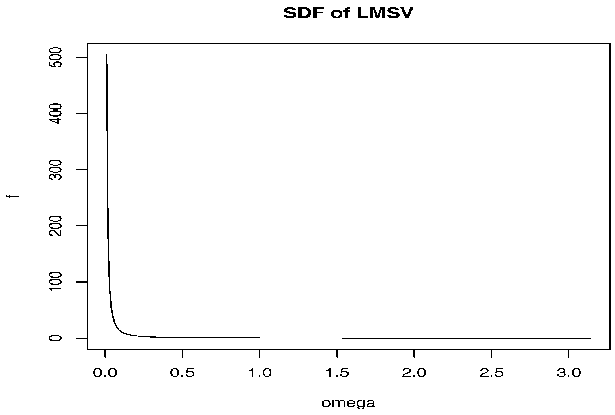
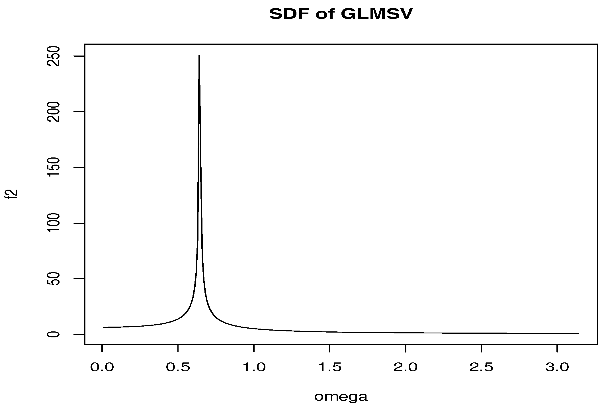
The lemma shows that the spectrum of $\left\{U_t\right\}$ behaves like that of $\left\{X_t\right\}$ near the Gegenbauer frequency, ${\omega }_g.$ We illustrate this for three important cases by taking $\varphi \left(L\right)=\theta \left(L\right)=1$ for simplicity.

Spectral Densities

• Standard LMSV when $\eta =1:$
  The sdf of $\left\{U_t\right\}$ is given by:

  $$f_U{\left(\omega \right)\sim [2\left(\sin (\omega /2)\right]}^{-4d}\frac{{\sigma }_v^2}{2\pi },-\pi <\omega <\pi ,$$

  (16)

  and is unbounded as $\omega \to 0$ when $0<d<1/2.$ The following diagram illustrates $f=f_U\left(\omega \right),d=0.4,{\sigma }_v^2=2$:
• GLMSV when $\left|\eta \right|<1:$
  The sdf of $\left\{U_t\right\}$ is given by:

  $$f_U\left(\omega \right)\sim {[4{(\cos \omega -\eta )}^2]}^{-d}\frac{{\sigma }_v^2}{2\pi },-\pi <\omega <\pi ,$$

  (17)

  and is unbounded as $\omega \to \arccos \left(\eta \right)$ (the Gegenbauer frequency, which is away from the origin) for $\left|\eta \right|<1$ and $0<d<1/2.$ The second diagram illustrates $f2=f_U\left(\omega \right),d=0.4,\eta =0.8,{\sigma }_v^2=2$:

5. Estimation and Forecasting

5.1. Spectral-Likelihood Estimator

Though the process $\left\{v_t\right\}$ is non-Gaussian, a reasonable estimation procedure is to maximize the quasi-likelihood, or the likelihood computed as if $\left\{v_t\right\}$ was Gaussian. For the LMSV models, the approaches of So (1999, 2002) and Doornik and Ooms (2003) enable us to compute the quasi-likelihood exactly, using the autocovariance functions up to order n. For the GLMSV model, it is not easy to calculate the exact autocovariances, but it is possible to obtain their approximate values with the use of the algorithm of McElroy and Holan (2012). Hence, the effectiveness of the QML estimation of this type depends on the accuracy of the approximation of the autocovariance functions. Rather than the approximate approach, we suggest a spectral domain estimator, which was used in estimating the GLSMV model by Artiach and Arteche (2012).

The spectral-likelihood (SL) estimator is obtained by minimizing:

$$\mathcal{L}\left(\lambda \right)=\frac{2\pi }{n}\sum _{j=1}^{[n/2]}\left[\log \left(f_U\left({\omega }_j\right)\right)+\frac{I_n\left({\omega }_j\right)}{f_U\left({\omega }_j\right)}\right]\times \mathbf{1}\left({\omega }_j\ne \arccos \left(\eta \right)\right),$$

(18)

where $\lambda ={(\delta ,{\eta }^{\prime })}^{\prime }$ and $\delta ={(d,{\varphi }_1,\dots ,{\varphi }_p,{\theta }_1,\dots ,{\theta }_q,{\sigma }_v,{\sigma }_{ϵ})}^{\prime }$ are the vectors of unknown parameters, $\mathbf{1}(·)$ is an indicator function which takes one if the condition is satisfied, and otherwise zero, $[·]$ denotes the integer part, ${\omega }_j=2\pi j/n$ is the jth Fourier frequency, and

$$I_n\left({\omega }_j\right)=\frac{1}{2\pi n}{\left|\sum _{t=1}^n{x}_t\exp (-i{\omega }_{j}t)\right|}^2,j=1,\cdots ,[n/2].$$

This technique is originally suggested by Breidt et al. (1998) for estimating the LMSV model. If we know the value of $\eta$ a priori, we should omit the observation which corresponds to $\omega =\arccos \left(\eta \right)$.

For estimating $\eta$, it is straightforward to show from Chung (1996a, 1996b) and Peiris and Asai (2016) that:

$$n(\widehat{\eta }-{\eta }_0)\stackrel{\mathcal{L}}{⟶}\frac{K\sin \left({\omega }_g\right)}{d}{Y}_0\mathrm{if}\left|\eta \right|<1\mathrm{and}d\ne 0,$$

(19)

where $K=E\left({\sigma }_t^{-2}\right)+2{\sum }_{j=1}^{\infty }{\phi }_{\sigma }\left(j\right)E({ϵ}_{t-i}^2/{\sigma }_t^4)$, $Y_0$ is a random variable defined as

$$Y_0\equiv \frac{{\int }_0^1{\tilde{W}}_{1}d{W}_2-{\int }_0^1{W}_{1}d{\tilde{W}}_2}{{\int }_0^1{\tilde{W}}_1^2\left(r\right)dr+{\int }_0^1{W}_1^2\left(r\right)dr},$$

and $({\tilde{W}}_1\left(t\right),{\tilde{W}}_2\left(t\right))$ and $(W_1\left(t\right),W_2\left(t\right))$ are two independent Brownian motions with mean zero and covariance,

$$t\left(\begin{array}{cc}E\left({\sigma }_t^2\right)& 1\\ 1& K\end{array}\right).$$

Furthermore,

$$n^2(\widehat{\eta }\mp 1)\stackrel{\mathcal{L}}{⟶}\pm \frac{K}{2d}{Y}_1\mathrm{if}\eta =\pm 1\mathrm{and}d\ne 0,$$

(20)

where $Y_1$ is a random variable defined as

$$Y_1\equiv \frac{{\int }_0^1\left\{{\int }_0^r{W}_1\left(s\right)ds\right\}d{W}_2\left(r\right)}{{\int }_0^1{\left\{{\int }_0^r{W}_1\left(s\right)ds\right\}}^{2}dr}.$$

Apart from $\eta$, Zaffaroni (2009) showed that the SL estimator, $\widehat{\lambda }$, is consistent, and:

$$\sqrt{T}(\widehat{\lambda }-{\lambda }_0)\stackrel{d}{⟶}N\left(0,W^{-1}U{\left(W^{*}\right)}^{-1}\right),$$

where ${\lambda }_0$ is the true value,

$$\begin{array}{cc}\hfill W& =\frac{\partial R\left(\lambda \right)}{\partial {\lambda }^{\prime }},\hfill \\ \hfill R\left(\lambda \right)& =\frac{\partial }{\partial \lambda }{\int }_{-\pi }^{\pi }\log f_U(\omega ;\lambda )d\omega -{\int }_{-\pi }^{\pi }\left[\frac{\partial }{\partial \lambda }\log f_U(\omega ;\lambda )\right]d\omega ,\hfill \\ \hfill U& =4\pi {\int }_{-\pi }^{\pi }\left[\frac{\partial }{\partial \lambda }\log f_U(\omega ;\lambda )\right]\left[\frac{\partial }{\partial {\lambda }^{\prime }}\log f_U(\omega ;\lambda )\right]d\omega \hfill \\ & +{\left(2\pi \right)}^3{\int }_{-\pi }^{\pi }{\int }_{-\pi }^{\pi }\left[\frac{\partial }{\partial \lambda }\log f_U({\omega }_1;\lambda )\right]\left[\frac{\partial }{\partial {\lambda }^{\prime }}\log f_U({\omega }_2;\lambda )\right]\hfill \\ & \times Q^e({\omega }_1,{\omega }_2,-{\omega }_2)d{\omega }_{1}d{\omega }_2,\hfill \end{array}$$

and $Q^e({\omega }_1,{\omega }_2,{\omega }_3)$ is the fourth-order cumulant spectral density of $e_t$, defined by (14). Furthermore, the SL estimator has the same limiting distribution as the QML estimator in the time domain. In practice, the second term of U can be estimated by the approach of Taniguchi (1982) (see chp. 5 of Taniguchi and Kakizawa (2000) and Zaffaroni (2009) for the general justification of the SL estimator). Zaffaroni (2009) shows the consistency and asymptotic normality of the SL estimator for conditional and stochastic volatility models with both short and long range dependencies.

Following Gray et al. (1989), Chung (1996a, 1996b), and Artiach and Arteche (2012), we use the grid search procedure for different values of $\eta$ over the range $[-1,1]$ for minimizing (18).

5.2. Finite Sample Properties

We conducted Monte Carlo experiments for investigating the finite sample properties of the SL estimator. The parameter values for $X_t$ are specified as:

$$(\mu ,\sigma ,\varphi ,d,\eta )=\left\{\begin{array}{cc}(0,0.199,0.98,0,1)\hfill & \mathrm{for}\mathrm{AR}\left(1\right)\hfill \\ (0,0.572,0.30,0.2,1)\hfill & \mathrm{for}\mathrm{ARFIMA}(1,2d,0)\hfill \\ (0,0.520,0.30,0.4,0.7)\hfill & \mathrm{for}\mathrm{GARMA}(1,d,0),\mathrm{Case}1\hfill \\ (0,0.675,0.70,0.3,0.3)\hfill & \mathrm{for}\mathrm{GARMA}(1,d,0),\mathrm{Case}2.\hfill \end{array}\right.$$

In the parameter settings, all the variances of $X_t$ are equal to one. Note that the standard deviation of ${ϵ}_t$ is ${\sigma }_{ϵ}=\pi /\sqrt{2}=2.221$, which is greater than twice the standard deviation of $X_t$. We consider sample sizes $n=\{1024,2048\}$, with $R=2000$ replications. For the AR and ARFIMA models, the structure ${(1-2\eta L+L^2)}^d$ implies that the estimate of $\eta$ can take any value when the estimate of d is close to zero.

Table 1 shows the finite sample performances of the SL estimator for the GARMA model. The bias for the estimator of d is negligible for both $n=1024$ and $n=2048$. The bias for $\eta$ is negligible when $d>0$, and it is meaningless if $d=0$. As noted before, when the true value of d is zero, the estimates of $\eta$ can take any values. The results for $d=0$ show that the estimates of $\eta$ are close to 0.7, and the RMSE has no major change with respect to the sample size. The bias for the estimates of $\mu$ and $\varphi$ are negligible. The estimator of ${\sigma }_{ϵ}$ has a downward bias, while that of $\sigma$ is biased upward. The result may come from the difference in the sizes of the parameters. The biases for ${\sigma }_{ϵ}$ and $\sigma$ become small as the sample size increases. For all the parameters, except for the meaningless case of $\eta$, the bias, standard deviation, and RMSE decrease as the sample size increases. Next we support the above findings using real data.

Table 1. Finite Sample Performance of the SL Estimator of GLMSV.

DGP	Parameters
	$\mathit{\mu }$	${\mathit{\sigma }}_{\mathit{ϵ}}$	$\mathit{\sigma }$	$\mathit{\varphi }$	$\mathit{d}$	$\mathit{\eta }$
AR(1)
True	0	2.221	0.199	0.98	0	1
$n=1024$	0.0091	2.1201	0.4863	0.9693	−0.1086	0.8972
	(0.2967)	(0.1901)	(0.4455)	(0.0305)	(0.3847)	(0.0830)
	[0.2967]	[0.2152]	[0.5297]	[0.0323]	[0.3993]	[0.1320]
$n=2048$	0.0011	2.1666	0.4047	0.9753	−0.0869	0.8986
	(0.2170)	(0.1137)	(0.3361)	(0.0119)	(0.3590)	(0.0797)
	[0.2168]	[0.1261]	[0.3938]	[0.0128]	[0.3691]	[0.1289]
ARFIMA(1,2d,0)
True	0	2.221	0.572	0.30	0.2	1
$n=1024$	0.0034	2.0796	0.5907	0.8551	0.1004	0.8901
	(0.4011)	(0.3942)	(0.6551)	(0.2127)	(0.3359)	(0.0824)
	[0.4007]	[0.4185]	[0.6547]	[0.5944]	[0.3500]	[0.1373]
$n=2048$	0.0063	2.2014	0.4303	0.8939	0.1568	0.9003
	(0.3394)	(0.1618)	(0.4617)	(0.1983)	(0.2928)	(0.0870)
	[0.3391]	[0.1629]	[0.4826]	[0.6261]	[0.2957]	[0.1322]
GARMA(1,d,0), Case 1
True	0	2.221	0.520	0.30	0.4	0.7
$n=1024$	0.0027	1.9444	0.9212	0.0988	0.3301	0.6984
	(0.0684)	(0.5856)	(0.5432)	(0.3501)	(0.1072)	(0.0307)
	[0.0684]	[0.6473]	[0.6749]	[0.4035]	[0.1280]	[0.0307]
$n=2048$	−0.0017	2.0965	0.7608	0.1693	0.3572	0.7005
	(0.0564)	(0.3353)	(0.4068)	(0.3143)	(0.0797)	(0.0052)
	[0.0564]	[0.3575]	[0.4724]	[0.3401]	[0.0904]	[0.0053]
GARMA(1,d,0), Case 2
True	0	2.221	0.675	0.70	0.3	0.3
$n=1024$	0.0037	2.0348	0.8180	0.6441	0.2668	0.3016
	(0.0871)	(0.5725)	(0.5207)	(0.2018)	(0.1481)	(0.0937)
	[0.0871]	[0.6016]	[0.5395]	[0.2092]	[0.1516]	[0.0936]
$n=2048$	−0.0014	2.1928	0.7022	0.6847	0.2905	0.3006
	(0.0696)	(0.2076)	(0.2269)	(0.1099)	(0.0747)	(0.0459)
	[0.0696]	[0.2094]	[0.2283]	[0.1109]	[0.0752]	[0.0458]

Note: Entries show the means of the SL estimates. Standard errors are in parentheses, and root mean squared errors are in brackets.

5.3. Estimating and Forecasting Volatility

We introduce an algorithm of Harvey (1998) regarding signal extraction and forecasting of long memory plus noise processes. Define $\mathit{U}={(U_1,\dots ,U_n)}^{\prime }$, ${\mathit{X}}^{*}={(X_1-\mu ,\dots ,X_n-\mu )}^{\prime }$, and $\mathit{ϵ}={({ϵ}_1,\dots ,{ϵ}_n)}^{\prime }$, in order to obtain:

$$\mathit{U}=(c+\mu ){\mathbf{1}}_n+{\mathit{X}}^{*}+\mathit{ϵ},$$

where ${\mathbf{1}}_n$ is an $n\times 1$ vector of ones. Then, the minimum mean square linear estimator of X is given by:

$${\tilde{\mathit{X}}}^{*}=(I_n-{\sigma }^2{\mathit{V}}^{-1})\left\{\mathit{U}-(c+\mu ){\mathbf{1}}_n\right\},$$

where $\mathit{V}={\mathit{V}}_X+{\sigma }^2{I}_n$, and ${\mathit{V}}_X$ denotes the covariance matrix of ${\mathit{X}}^{*}$. As noted in Section 5.1, ${\mathit{V}}_X$ can be approximated by the algorithm of McElroy and Holan (2012) (see the Appendix A for details). Harvey (1998) recommends using the volatility estimate:

$${\tilde{\sigma }}_t^2={\tilde{\sigma }}_{\tilde{Y}}^2\exp \left({\tilde{X}}_t^{*}\right),$$

where ${\tilde{\sigma }}_{\tilde{Y}}^2=n^{-1}{\sum }_{t=1}^n{\tilde{Y}}_t^2$, and ${\tilde{Y}}_t=Y_t\exp (-0.5{\tilde{X}}_t^{*})$ are the heteroskedasticity-corrected observations.

For predicting the observations on $U_t$ for $t=n+1,\dots ,n+h$, denote ${\mathit{U}}_h$ as the $h\times 1$ vector of predicted values. Then the corresponding MMSLEs are given by:

$${\tilde{\mathit{U}}}_h=(\mu +c){\mathbf{1}}_h+\mathit{R}{\mathit{V}}^{-1}\left\{\mathit{U}-(\mu +c){\mathbf{1}}_n\right\},$$

where R is the $h\times n$ matrix of covariances between ${\mathit{U}}_h$ and U. Using ${\tilde{\mathit{X}}}_h={\tilde{\mathit{U}}}_h-(\mu +c){\mathbf{1}}_h$, the predictions of ${\sigma }_{n+j}^2$$(j=1,\dots ,h)$ are given by exponentiating the elements of ${\tilde{\mathit{X}}}_h$, and multiplying by ${\tilde{\sigma }}_{\tilde{Y}}^2$.

6. Empirical Analysis

6.1. Data and Preliminary Results

The empirical analysis focuses on estimating and forecasting the GLMSV model for three sets of exchange rate data, namely YEN/USD, EUR/USD, and GBP/USD. The sample period is from 4 October 2005 to 25 November 2015, giving 2549 observations. We calculated the returns series, $R_t=\log P_t-\log P_{t-1}$, where $P_t$ is the closing price on day t. We use the first $n=2048$ returns for estimating the GLMSV models, and the remaining 500 series for forecasting. The estimation period includes the global financial crisis. Table 2 presents descriptive statistics for the whole sample. As our interest is on volatility, we use the mean subtracted returns, $Y_t=R_t-\overline{R}$.

Table 2. Descriptive Statistics for Exchange Rate Returns.

Data	Mean	Std. Dev.	Skewness	Kurtosis
YEN/USD	0.0028	0.6617	−0.3225	8.1747
EUR/USD	−0.0045	0.6383	0.1717	5.9683
GBP/USD	−0.0060	0.6163	−0.3377	9.6188

As a preliminary analysis, we estimated the new generalized fractionally integrated EGARCH (GIEGARCH) model, defined by:

$$\begin{array}{c}{Y}_t=\sqrt{h_t}{\xi }_t,{\xi }_t\sim IID(0,1),\hfill \\ \varphi \left(L\right){(1-2\eta L+L^2)}^d(\log h_t-\mu )=\theta \left(L\right)\zeta \left({\xi }_{t-1}\right),\hfill \end{array}$$

where $\zeta \left({\xi }_t\right)$ is the generalized return, and $\varphi \left(L\right)$ and $\theta \left(L\right)$ are defined in Section 3. Following Hansen et al. (2012), we consider the second-order Hermite polynomial for the error term, as:

$$\zeta \left({\xi }_t\right)={\gamma }_1{\xi }_t+{\gamma }_2({\xi }_t^2-E\left({\xi }_t^2\right)).$$

Assuming that ${\xi }_t$ has finite fourth moment, it is straightforward to show $E\left[\zeta \left({\xi }_t\right)\right]=0$ and $V\left[\zeta \left({\xi }_t\right)\right]<\infty$. When $\eta =1$, the new GIEGARCH(p,d,q; $\eta$) model reduces to the class of the FIEGARCH(p,$2d$,q) model of Bollerslev and Mikkelsen (1996). Following Bollerslev and Mikkelsen (1996), we truncate the MA(∞) representation of the GARMA process of log-volatility as:

$$\log h_t=\mu +\sum _{j=0}^J{\tilde{\psi }}_j\zeta \left({\xi }_{t-1-j}\right),$$

where ${\tilde{\psi }}_j$ is the jth coefficient of the polynomial $\tilde{\psi }\left(z\right)={(1-2\eta z+z^2)}^{-d}\varphi {\left(z\right)}^{-1}\theta \left(z\right)$, with ${\tilde{\psi }}_0=1$. We calculate the value of ${\tilde{\psi }}_j$ by the approximating technique of McElroy and Holan (2012) up to $J=1000$ (see the Appendix A).

In addition to the FIEGARCH and GIEGARCH models, we estimated the GARCH model with the conditional volatility equation:

$$h_t=w+\alpha Y_{t-1}^2+\beta h_{t-1},$$

as a benchmark.

Table 3 gives the QML estimates of the GARCH model. As a typical result, the estimates of $\alpha +\beta$ is close to one, indicating a possible long range dependence in volatility. Table 4 shows the QML estimates of the FIEGARCH(1,$2d$,0) and GIEGARCH(1,d,0; $\eta$) models. For the FIEGARCH model, the estimates of d indicate that the conditional log-volatility, $\log h_t$, has long range dependence. The estimates of ${\gamma }_1$ are negative, while those of ${\gamma }_2$ are positive. The estimates of $\varphi$ are located in the interval (−0.25, −0.1). Except for the estimates of ${\gamma }_1$ for the EUR/USD return, all parameter estimates are significant at the five percent level. These estimates are similar to the values obtained in the literature.

Table 3. QML Estimates of GARCH Model.

Parameters	YEN/USD	EUR/USD	GBP/USD
w	0.0045	0.0010	0.0018
	(0.0010)	(0.0005)	(0.0008)
$\alpha$	0.0342	0.0329	0.0394
	(0.0036)	(0.0046)	(0.0056)
$\beta$	0.9565	0.9647	0.9556
	(0.0047)	(0.0044)	(0.0065)

Note: Standard errors are in parentheses.

Table 4. QML Estimates of FIEGARCH and GIEGARCH Models.

Parameters	YEN/USD		EUR/USD		GBP/USD
	FIEGARCH	GIEGARCH	FIEGARCH	GIEGARCH	FIEGARCH	GIEGARCH
$\mu$	−0.7736	−0.8589	−0.7916	−0.9170	−0.8771	−1.0338
	(0.0474)	(0.0427)	(0.0715)	(0.0776)	(0.0809)	(0.0760)
$\varphi$	−0.1084	0.9749	−0.2401	0.9854	−0.2006	0.9881
	(0.0278)	(0.0034)	(0.0509)	(0.0014)	(0.0379)	(0.0019)
${\gamma }_1$	−1.1991	−0.0415	−0.2439	−0.0119	−0.7873	−0.0229
	(0.3571)	(0.0064)	(0.1325)	(0.0036)	(0.2147)	(0.0042)
${\gamma }_2$	0.7254	0.0321	0.5071	0.0140	0.4779	0.0108
	(0.2696)	(0.0043)	(0.1496)	(0.0023)	(0.1727)	(0.0027)
d	0.1491	0.3350	0.2368	0.4988	0.2495	0.4996
	(0.0345)	(0.0750)	(0.0365)	(0.0854)	(0.0431)	(0.0624)
$\eta$	1	0.3892	1	0.8583	1	0.8570
		(0.0026)		(0.0014)		(0.0006)
${\omega }_g$	0	1.1710	0	0.5388	0	0.5414

Note: Standard errors are in parentheses. The Gegenbauer frequency is given by ${\omega }_g=\arccos \left(\eta \right)$.

The estimates of d in the GIEGARCH model are about twice of those for the FIEGARCH model. The estimates of $\eta$ are positive, and the estimates of $\varphi$ are close to one. The estimates of ${\gamma }_1$ are negative, while those of ${\gamma }_2$ are positive. All parameter estimates are significant at the five percent level. As the estimates of $\eta$ are significantly different from one, the estimates of the Gegenbauer frequency, ${\omega }_g=\arccos \left(\eta \right)$, are different from zero.

6.2. Estimates and Forecasts for the GLMSV Model

In the following, we show the empirical results for the GLMSV models as compared with those of the GIEGARCH model.

Table 5 gives the SL estimates of the GLMSV model. The estimates of d and $\varphi$ are close to the values of the GIEGARCH model. Compared with the GIEGARCH model, the estimates of $\eta$ are higher. The estimates of $\mu$ are different from those of the GIEGARCH model, and the differences may arise from the statistical flexibility of the class of SV models compared with their conditional heteroskedasticity counterparts. All estimates are significant at the five percent level. As the estimates of $\eta$ are significantly different from one, the estimates of the Gegenbauer frequency ${\omega }_g=\arccos \left(\eta \right)$ are different from zero.

Table 5. Estimates of GLMSV for Daily Currency Returns.

Parameters	YEN/USD	EUR/USD	GBP/USD
$\mu$	−1.2366	−1.2030	−1.3069
	(0.0579)	(0.0544)	(0.0538)
${\sigma }_{ϵ}$	2.5173	2.3482	2.2844
	(0.0414)	(0.0384)	(0.0368)
$\sigma$	0.0868	0.1621	0.0974
	(0.0350)	(0.0378)	(0.0311)
$\varphi$	0.9872	0.9939	0.9980
	(0.0066)	(0.0042)	(0.0039)
d	0.3173	0.4702	0.4987
	(0.1475)	(0.1029)	(0.1869)
$\eta$	0.8032	0.9597	0.8400
	(0.0001)	(0.0003)	(0.0009)
${\omega }_g$	0.6381	0.2849	0.5735

Note: Standard errors are in parentheses. The Gegenbauer frequency is given by ${\omega }_g=\arccos \left(\eta \right)$.

As explained previously, we use the last 500 observations for the rolling-window forecasting analysis, based on the approach in the previous section. First, we report the estimates of the Mincer–Zarmowitz (MZ) regression, given by:

$$Y_t^2=a+b{\widehat{\sigma }}_{t|t-1}^2+e_t,t=n+1,\dots ,n+500,$$

where ${\widehat{\sigma }}_{t|t-1}^2$ is the one-step ahead forecast of ${\sigma }_t^2$ on day t. Table 6 presents the results of OLS estimation with heteroskedasticity and autocorrelation consistent standard errors. For all three data sets, the GLMSV model has the highest $R^2$. We should note that the simple GARCH model has the second highest $R^2$ for two series.

Table 6. Results for MZ Reression.

Data	Parameter	GARCH	FIEGARCH	GIGARCH	GLMSV
YEN/USD	a	0.0859	0.0715	0.0404	−0.2356
		(0.0676)	(0.0660)	(0.0687)	(0.0898)
	b	0.5887	0.5906	0.7116	1.5406
		(0.1951)	(0.1765)	(0.1933)	(0.2596)
	S.E.	0.6496	0.6482	0.6467	0.6335
	$R^2$	0.1609	0.1644	0.1682	0.2020 †
EUR/USD	a	0.0329	−0.0493	−0.0631	0.1012
		(0.0448)	(0.0652)	(0.0563)	(0.0360)
	b	0.8955	1.0968	1.1251	0.2704
		(0.1116)	(0.1729)	(0.1438)	(0.0307)
	S.E.	0.5624	0.5748	0.5640	0.5560
	$R^2$	0.3226	0.2922	0.3187	0.3379 †
GBP/USD	a	0.0314	0.0464	0.0052	−0.4764
		(0.0317)	(0.0435)	(0.0398)	(0.1018)
	b	0.7768	0.5747	0.7346	1.4038
		(0.1445)	(0.1704)	(0.1520)	(0.2140)
	S.E.	0.3090	0.3143	0.3107	0.3050
	$R^2$	0.2950	0.2708	0.2875	0.3134 †

Note: Heteroskedasticity and autocorrelation consistent standard errors are given in parenthesis. ‘†’ denotes the highest value of $R^2$.

Secondly, we compare the forecasts using the robust and homogeneous loss function suggested by Patton (2011), defined by:

$$L({\widehat{\sigma }}^2,h)=\left\{\begin{array}{cc}\frac{1}{c(c-1)}({\widehat{\sigma }}^{2c}-h^c)-\frac{1}{c-1}{h}^{c-1}({\widehat{\sigma }}^2-h)\hfill & (c\notin \{0,1\left\}\right)\hfill \\ h-{\widehat{\sigma }}^2+{\widehat{\sigma }}^2\log \frac{{\widehat{\sigma }}^2}{h}\hfill & (c=1)\hfill \\ \frac{{\widehat{\sigma }}^2}{h}-\log \frac{{\widehat{\sigma }}^2}{h}-1\hfill & (c=0),\hfill \end{array}\right.$$

where c is the degree of homogeneity, h is the proxy of volatility ($h=Y^2$), and ${\widehat{\sigma }}^2$ is the forecast of volatility. The general loss function reduces to the mean squared error (MSE) when $c=2$, while it is equivalent to the the loss function based on the quasi-log-likelihood (QLIKE) when $c=0$. Table 7 shows the average of the loss function for the cases $c=0,1,2$. For all three series, two of three loss functions chose the GLMSV model, while the remaining one selects the GARCH model.

Table 7. Comparison of Volatility Forecasts.

Data	Loss Function	GARCH	FIEGARCH	GIGARCH	GLMSV
YEN/USD	$c=2$ (MSE)	0.2129	0.2137	0.2106	0.1594 †
	$c=1$	0.4661	0.5006	0.4812	0.4232 †
	$c=0$ (QLIKE)	284.45 †	342.79	299.66	320.26
EUR/USD	$c=2$ (MSE)	0.1578	0.1648	0.1588	0.0849 †
	$c=1$	0.4565 †	0.5245	0.5020	0.5787
	$c=0$ (QLIKE)	362.20	497.04	476.01	354.85 †
GBP/USD	$c=2$ (MSE)	0.0479	0.0514	0.0502	0.0089 †
	$c=1$	0.2995	0.3804	0.3773	0.1983 †
	$c=0$ (QLIKE)	35,926 †	41,066	37,279	36,204

Note: ‘†’ denotes the smallest value.

Thirdly, we calculated the Value-at-Risk (VaR) thresholds, assuming normality of ${\xi }_t$. Combined with the one-day-ahead forecasts of log-volatility, we computed the 1 and 5 percent VaR thresholds as $-2.326{\widehat{\sigma }}_{n+1}^2$ and $-1.645{\widehat{\sigma }}_{n+1}^2$, respectively, fixing the sample size as $n=2048$. In order to assess the estimated VaR thresholds, we use the GMM duration-based tests developed by Candelon et al. (2011), which works with the J-statistic based on the moments defined by the orthonormal polynomials that are associated with the geometric distribution. The conditional coverage test and independence test based on q orthonormal polynomials have the asymptotic ${\chi }_q^2$ and ${\chi }_{q-1}^2$ distributions under their respective null distributions. The unconditional coverage test is given as a special case of the conditional coverage test, with $q=1$. Table 8 shows the percentage of VaR violations and test results for the GARCH, FIEGARCH, GIEGARCH and GLMSV models. For the FIEGARCH model, some of the test statistics are rejected at the five percent significance level. On the other hand, for the GARCH, GIEGARCH, and GLMSV models, the tests do not reject the null hypothesis at the 5% and 1% VaR thresholds, thereby indicating that the estimated VaR thresholds are satisfactory.

Table 8. Backtesting VaR Thresholds for One-Step-Ahead Forecasts.

Data	VaR	GARCH		FIEGARCH		GIEGARCH		GLMSV
		5%	1%	5%	1%	5%	1%	5%	1%
YEN/USD	PV	0.036	0.008	0.034	0.004	0.036	0.004	0.0040	0.010
	UC	0.6540	0.3168	0.9752	0.5989	0.5029	1.5034	0.0733	1.2558
		[0.4187]	[0.5735]	[0.3234]	[0.4390]	[0.4782]	[0.2201]	[0.7866]	[0.2625]
	IND	1.7393	1.0694	8.1759	0.9347	2.1775	1.1999	5.2835	1.6877
		[0.7836]	[0.8991]	[0.0853]	[0.9195]	[0.732]	[0.8781]	[0.2594]	[0.7930]
	CC	5.4979	3.3522	76.331 *	2.0605	5.4058	3.7080	7.2375	1.6877
		[0.3582]	[0.6459]	[0.0000]	[0.8407]	[0.3684]	[0.5922]	[0.2036]	[0.8905]
EUR/USD	PV	0.036	0.008	0.058	0.010	0.054	0.008	0.044	0.018
	UC	0.6540	0.3168	20866	0.3457	0.3174	0.0097	0.6177	2.0001
		[0.4187]	[0.5735]	[0.1486]	[0.5566]	[0.5732]	[0.9214]	[0.4319]	[0.1573]
	IND	1.7393	1.0694	1.3895	1.7610	0.0726	0.2397	3.5391	0.9180
		[0.7836]	[0.8991]	[0.8460]	[0.7796]	[0.9994]	[0.9934]	[0.4720]	[0.9220]
	CC	5.4979	3.3522	3.0081	1.7610	0.3424	0.1625	6.6769	2.8541
		[0.3582]	[0.6459]	[0.6987]	[0.8811]	[0.9968]	[0.9995]	[0.2458]	[0.7225]
GBP/USD	PV	0.068	0.016	0.048	0.004	0.050	0.004	0.052	0.012
	UC	2.7886	2.8064	0.0193	04137	0.0281	2.0368	1.7100	2.3767
		[0.0949]	[0.0939]	[0.8894]	[0.5201]	[0.8669]	[0.1535]	[0.1910]	[0.1232]
	IND	1..3485	1.7954	18.555 *	0.8417	1.0782	1.2781	7.1894	2.7581
		[0.8531]	[0.7733]	[0.0010]	[0.9328]	[0.8977]	[0.8651]	[0.1262]	[0.5991]
	CC	2.9997	4.0075	23.801 *	1.7850	1.0782	4.6977	3.9607	3.8607
		[0.7000]	[0.5483]	[0.0002]	[0.8780]	[0.9560]	[0.4539]	[3.9607]	[3.8607]

Note: PV denotes the percentage of violations, which is the percentage of days when returns are less than the VaR threshold. UC, IND, and CC are the generalized method of moments duration-based tests for unconditional coverage, independence and conditional coverage, developed by Candelon et al. (2011). The number of orthonormal polynomials is set to 5. p values are in brackets. ‘*’ denotes significance at 5% level.

By the three kinds of measures of forecasting performance, we found that the GLMSV model always outperforms the FIEGARCH and GIEGARCH models for the period includes the global financial crises. We also found that the simple GARCH model is the second best model.

7. Concluding Remarks

In this paper, we considered a generalized long memory volatility (GLMSV) model, based on the GARMA(p,d,q; $\eta$) process, and examined the statistical properties. We discussed theoretical background of the spectral likelihood (SL) estimation method, for which the asymptotic distribution is the same as that of the QML estimator. Then we conducted Monte Carlo experiments for investigating the finite sample properties of the SL estimator, and found that the finite sample biases are negligible for $n=2048$.

In addition, we estimated the GARCH, FIEGARCH, GIEGARCH, and GLMSV models, using three exchange rate returns for YEN/USD, EUR/USD, and GBP/USD. The empirical results supported long memory for log-volatility, and also showed a non-zero Gegenbauer frequency. Furthermore, the specification of generalized long memory improved satisfactory the out-of-sample forecasts for the MZ regression, the loss functions, and the VaR thresholds, which shows that the GLMSV model is a useful addition to the existing models in the literature.

References

- Andersen, Torben G., Tim Bollerslev, Francis X. Diebold, and Paul Labys. 2001. The distribution of realized exchange rate volatility. Journal of the American Statistical Association 96: 42–55. [Google Scholar] [CrossRef]
- Andersen, Torben G., Tim Bollerslev, Francis X. Diebold, and Paul Labys. 2003. Modeling and forecasting realized volatility. Econometrica 71: 529–626. [Google Scholar] [CrossRef]
- Artiach, Miguel, and Josu Arteche. 2012. Doubly Fractional Models for Dynamic Heteroscedastic Cycles. Computational Statistics & Data Analysis 56: 2139–58. [Google Scholar]
- Asai, Manabu, Michael McAleer, and Marcelo C. Medeiros. 2012. Asymmetry and long memory in volatility modeling. Journal of Financial Econometrics 10: 495–512. [Google Scholar] [CrossRef]
- Baillie, Richard T., Tim Bollerslev, and Hans Ole Mikkelsen. 1996. Fractionally integrated generalized autoregressive conditional heteroskedasticity. Journal of Econometrics 74: 3–30. [Google Scholar] [CrossRef]
- Barndorff-Nielsen, Ole E., and Neil Shephard. 2002. Econometric analysis of realized volatility and its use inestimating stochastic volatility models. Journal of the Royal Statistical Society, Series B 64: 253–80. [Google Scholar] [CrossRef]
- Bollerslev, Tim, and Hao Zhou. 2002. Estimating stochastic volatility diffusion using conditional moments of integrated volatility. Journal of Econometrics 109: 33–65. [Google Scholar] [CrossRef]
- Bollerslev, Tim, and Hans Ole Mikkelsen. 1996. Modeling and pricing long-memory in stock market volatility. Journal of Econometrics 73: 151–84. [Google Scholar] [CrossRef]
- Bordignon, Silvano, Massimiliano Caporin, and Francesco Lisi. 2007. Generalised Long-memory GARCH Models for Intra-daily Volatility. Computational Statistics & Data Analysis 51: 5900–12. [Google Scholar]
- Breidt, F. Jay, Nuno Crato, and Pedro de Lima. 1998. The detection and estimation of long memory. Journal of Econometrics 83: 325–48. [Google Scholar] [CrossRef]
- Candelon, Bertrand, Gilbert Colletaz, Christophe Hurlin, and Sessi Tokpavi. 2011. Backtesting value-at-risk: A GMM duration-based approach. Journal of Financial Econometrics 9: 314–43. [Google Scholar] [CrossRef]
- Chung, Ching-Fan. 1996a. Estimating a generalized long memory process. Journal of Econometrics 73: 237–59. [Google Scholar] [CrossRef]
- Chung, Ching-Fan. 1996b. A generalized fractionally integrated autoregressive moving-average process. Journal of Time Series Analysis 17: 111–40. [Google Scholar] [CrossRef]
- Clark, Peter K. 1973. A subordinated stochastic process model with fixed variance for speculative prices. Econometrica 41: 135–56. [Google Scholar] [CrossRef]
- Dissanayake, G., S. Peiris, and T. Proietti. 2016. State space modeling of Gegenbauer processes with long memory. Computational Statistics & Data Analysis 100: 115–30. [Google Scholar]
- Doornik, Jurgen A., and Marius Ooms. 2003. Computational aspects of maximum likelihood estimation of autoregressive fractionally integrated moving average models. Computational Statistics & Data Analysis 42: 333–48. [Google Scholar]
- Engle, Robert F. 1982. Autoregressive conditional heteroskedasticity with estimates of the variance of United Kingdom inflation. Econometrica 50: 987–1007. [Google Scholar] [CrossRef]
- Granger, C.W.J., and M. Morris. 1976. Time series modeling and interpretation. Journal of the Royal Statistical Society, Series A 139: 246–57. [Google Scholar] [CrossRef]
- Gray, Henry L., Nien-Fan Zhan, and Wayne A. Woodward. 1989. On generalized fractional processes. Journal of Time Series Analysis 10: 233–57. [Google Scholar] [CrossRef]
- Hansen, Peter Reinhard, Zhuo Huang, and Howard Howan Shek. 2012. Realized GARCH: A Complete Model of Returns and Realized Measures of Volatility. Journal of Applied Econometrics 27: 877–906. [Google Scholar] [CrossRef]
- Harvey, Andrew C. 1998. Long memory in stochastic volatility. In Forecasting Volatility in Financial Markets. Edited by J. Knight and S. Satchell. Oxford: Butterworth-Haineman, pp. 307–20. [Google Scholar]
- Koopman, Siem Jan, Borus Jungbacker, and Eugenie Hol. 2005. Forecasting daily variability of the S&P 100 stock index using historical, realised and implied volatility measurements. Journal of Empirical Finance 12: 445–75. [Google Scholar]
- McAleer, Michael. 2005. Automated inference and learning in modeling financial volatility. Econometric Theory 21: 232–61. [Google Scholar] [CrossRef]
- McElroy, Tucker S., and Scott H. Holan. 2012. On the computation of autocovariances for generalized Gegenbauer processes. Statistica Sinica 22: 1661–87. [Google Scholar] [CrossRef]
- Patton, Andrew J. 2011. Volatility forecast comparison using imperfect volatility proxies. Journal of Econometrics 160: 246–56. [Google Scholar] [CrossRef]
- Peiris, M. Shelton, and Manabu Asai. 2016. Generalized fractional processes with long memory and time dependent volatility revisited. Econometrics 4: 37. [Google Scholar] [CrossRef]
- Pong, Shiuyan, Mark B. Shackleton, Stephen J. Taylor, and Xinzhong Xu. 2004. Forecasting currency volatility: A comparison of implied volatilities and AR(FI)MA models. Journal of Banking and Finance 28: 2541–63. [Google Scholar] [CrossRef]
- Shephard, Neil. 2005. General introduction. In Stochastic Volatility. Edited by N. Shephard. Oxford: Oxford University Press, pp. 1–33. [Google Scholar]
- Shitan, Mahendran, and Shelton Peiris. 2008. Generalized autoregressive (GAR) model: A comparison of maximum likelihood and Whittle estimation procedures using a simulation study. Communications in Statistics—Theory and Methods 37: 560–70. [Google Scholar] [CrossRef]
- Shitan, Mahendran, and Shelton Peiris. 2013. Approximate asymptotic variance-covariance matrix for the Whittle estimators of GAR(1) parameters. Communications in Statistics—Theory and Methods 42: 756–70. [Google Scholar] [CrossRef] [Green Version]
- So, M.K.P. 1999. Time series with additive noise. Biometrika 86: 474–82. [Google Scholar] [CrossRef]
- So, M.K.P. 2002. Bayesian analysis of long memory stochastic volatility models. Sankhyā 24: 1–10. [Google Scholar]
- Taniguchi, Masanobu. 1982. On estimation of the integrals of the fourth order cumulant spectral density. Biometrika 69: 117–22. [Google Scholar] [CrossRef]
- Taniguchi, Masanobu, and Yosihihide Kakizawa. 2000. Asymptotic Theory of Statistical Inference for Time Series. New York: Springer. [Google Scholar]
- Taylor, Stephen J. 1982. Financial returns modeled by the product of two stochastic processes—A study of daily sugar prices 1961–1979. In Time Series Analysis: Theory and Practice. Edited by O. D. Anderson. Amsterdam: North-Holland, vol. 1, pp. 203–26. [Google Scholar]
- Taylor, Stephen J. 1986. Modelling Financial Time Series. Chichester: Wiley. [Google Scholar]
- Zaffaroni, Paolo. 2009. Whittle estimation of EGARCH and other exponential volatility models. Journal of Econometrics 151: 190–200. [Google Scholar] [CrossRef]