The Burr X Pareto Distribution: Properties, Applications and VaR Estimation
by
 , , and
Mustafa Ç. Korkmaz
1,* ,
,
Emrah Altun
2,
Haitham M. Yousof
3 ,
,
Ahmed Z. Afify
3 and
and
Saralees Nadarajah
4 1
Department of Measurement and Evaluation, Artvin Çoruh University, Artvin 08000, Turkey
2
Department of Statistics, Hacettepe University, Ankara 06800, Turkey
3
Department of Statistics, Mathematics and Insurance, Benha University, Benha 13511, Egypt
4
School of Mathematics, University of Manchester, Manchester M13 9PL, UK
*
Author to whom correspondence should be addressed.
J. Risk Financial Manag. 2018, 11(1), 1; https://doi.org/10.3390/jrfm11010001
Submission received: 31 October 2017
/
Revised: 30 November 2017
/
Accepted: 18 December 2017
/
Published: 21 December 2017
(This article belongs to the Special Issue Extreme Values and Financial Risk)
Abstract
:In this paper, a new three-parameter Pareto distribution is introduced and studied. We discuss various mathematical and statistical properties of the new model. Some estimation methods of the model parameters are performed. Moreover, the peaks-over-threshold method is used to estimate Value-at-Risk (VaR) by means of the proposed distribution. We compare the distribution with a few other models to show its versatility in modelling data with heavy tails. VaR estimation with the Burr X Pareto distribution is presented using time series data, and the new model could be considered as an alternative VaR model against the generalized Pareto model for financial institutions.
1. Introduction
The Pareto (P) distribution is very versatile, and a variety of uncertainties can be usefully modelled by it. It has several applications in actuarial science, economics, finance, life testing, survival analysis and telecommunications because of its heavy tail properties. The probability density function (pdf) and cumulative distribution function (cdf) of the P distribution are given (for ) by:
where is a scale parameter and is a shape parameter. This distribution is a special form of the Pearson Type VI distribution. Since the P distribution has a reversed-J pdf shape and a decreasing hazard rate function (hrf), it may sometimes be insufficient to model data. Generally, practical problems require a wider range of possibilities for the medium risk, for example when the lifetime data present a bathtub-shaped hrf, such as human mortality and machine life cycles. For this reason, researchers developed various extensions and modified forms of the P distribution to obtain a more flexible model with different numbers of parameters. Some of them can be cited as follows: Exponentiated P (EP) (Stoppa 1990; Gupta et al. 1998), Beta P (BP) (Akinsete et al. 2008), Kumaraswamy P (KwP) (Bourguignon et al. 2013), Kumaraswamy generalized P (Nadarajah and Eljabri 2013), P ArcTan (PAT) (Gómez-Déniz and Calderín-Ojeda 2015), exponentiated Weibull P (Afify et al. 2016) and Weibull P (WP) distributions (Tahir et al. 2016). On the other hand, Yousof et al. (2016) defined the cdf of the Burr X-G(BX-G) family (for ) by:
where is the shape parameter and () is a parameter vector. The BX-G density function becomes:
This generator can supply the flexibility of pdf and hrf to any baseline distribution model (Yousof et al. 2016).
In this paper, we introduce a new extended P distribution, called the Burr X Pareto (BXP) model, based on the BX-G family. With this idea, we construct the new BXP distribution as more flexible than the P distribution and provide a comprehensive description of some of its mathematical properties. We prove empirically that the BXP model provides better fits than some extensions and generalizations of the P, some of which have one extra model parameter, and the others have the same number of parameters, by means of two applications to real data. We hope that the new distribution will attract wider applications in reliability, engineering and other areas of research.
The rest of the paper is organized as follows. In Section 2, we define the BXP model. In Section 3, we provide a useful mixture representation for its pdf. In Section 4, we derive some of its general mathematical properties. Some estimation methods of the model parameters are performed in Section 5. In Section 6, simulation results to assess the performance of the proposed maximum likelihood estimation procedure are discussed. In Section 7, we provide two applications to real data to illustrate the importance and flexibility of the new family. Value-at-Risk estimation with the BXP distribution is presented in Section 8. Finally, some concluding remarks are presented in Section 9.
2. The New Model
In this section, we define the BXP model and provide some plots for its pdf and hrf. The BXP cdf is given by:
The pdf corresponding to (3) is given by:
Lemma 1 provides random number generations from the BXP and some relations and of the BXP distribution with the well-known Burr X and uniform distributions.
Lemma 1.
(a) If a random variable Y follows the Burr X distribution with shape parameter δ and scale parameter one, then the random variable follows the BXP distribution.
(b) If a random variable Y follows the uniform distribution on [0,1], then the random variable:
follows the BXP distribution.
Proof.
The proofs of (a) and (b) are obtained by the transformation method. ☐
The hrf, reversed hazard rate function and cumulative hazard rate function of are given, respectively, by:
and:
3. Expansions of pdf and cdf
In this section, we provide a very useful linear representation for the BXP density function. If and is a real non-integer, the power series holds:
Applying the power series to the term , Equation (6) becomes:
Consider the series expansion:
Equation (9) reveals that the density of X can be expressed as expansions of the EP densities. Therefore, several mathematical properties of the new family can be obtained by knowing those of the EP distribution. Similarly, the cdf of the BXP family can also be expressed as a mixture of EP cdfs given by:
where:
is the cdf of the EP family with power parameter .
4. Properties
In this section, we will provide some mathematical properties of the BXP distribution.
4.1. Moments
is the r-th ordinary moment of EP distribution with power parameter .
The j-th order central moment can be obtained by the following relationship:
where .
For the skewness and kurtosis coefficients, we have:
The values for mean, variance, and for selected values of and are shown in Table 1. We can say that the BXP model can be useful for various data modelling in terms of skewness and kurtosis.
4.2. Residual and Reversed Residual Life
The n-th moment of the residual life, say , , …, uniquely determines . The n-th moment of the residual life of X is given by:
Therefore,
where:
is the incomplete beta function.
The Mean Residual Life (MRL) function or the life expectation at age t defined by follows by setting in the last equation.
The n-th moment of the reversed residual life, say for and , … uniquely determines . We obtain:
Then, the n-th moment of the reversed residual life of X becomes:
The mean inactivity time (MIT) or mean waiting time is given by , and it can be obtained easily by setting in the above equation.
4.3. Order Statistics
Order statistics make their appearance in many areas of statistical theory and practice. Let be a random sample from the BXP of distributions, and let be the corresponding order statistics. The pdf of the i-th order statistic, say , can be written as:
The pdf of can be expressed as:
Then, the density function of the BXP order statistics is a mixture of EP densities. Based on the last equation, we note that the properties of follow from those properties of . For example, the moments of can be expressed as:
5. Estimation Methods
In this section, we consider the maximum likelihood, least square and weighted least square estimation of the parameters of the BXP distribution.
5.1. Maximum Likelihood Estimation
We consider the estimation of the unknown parameters of the BXP model from complete samples by the maximum likelihood method. The maximum likelihood estimators (MLEs) of the parameters of the BXP model are now discussed. Let be a random sample of this distribution with parameter vector . The log-likelihood function for is given by:
where .
The last equation can be also maximized either by using the different programs such as R (optim function), SAS (PROC NLMIXED) or by solving the nonlinear likelihood equations obtained by differentiating ℓ. We note that since the MLE of the parameter cannot be obtained in the usual way. Hence, the MLE of is the first order statistic (Johnson et al. 1994).
The components of the score vector, , are:
and:
where:
For fixed , the interval estimation of the model parameters requires the observed information matrix for . The multivariate normal distribution, under standard regularity conditions, can be used to provide approximate confidence intervals for the unknown parameters, where is the total observed information matrix evaluated at . Then, approximate confidence intervals for and can be determined by:
and , where is the upper -th percentile of the standard normal model.
5.2. Ordinary and Weighted Least Squares
In this section, we use the least square (LS) and weighted least square (WLS) estimators (Swain et al. 1988) to estimate the parameters of the BXP distribution. Let be the order statistics of a random sample of size n from the BXP defined in (4), then the least square estimators (LSEs) of the unknown parameters , and of the BXP distribution can be obtained by minimizing:
with respect to unknown parameters , and .
The weighted least square estimators (WLSEs) of the unknown parameters , and follow by minimizing:
with respect to unknown parameters , and .
6. Simulation Study
Here, we perform the simulation study for MLEs of the BXP distribution. We generate samples of sizes , 100, 200 from selected BXP distributions. The random numbers generation is simulated by:
where u is a uniform random number on [0,1]. We also calculate the empirical mean, standard deviations (sd), bias and mean square error (MSE) of the MLEs. The empirical bias and MSE are calculated by:
and:
respectively, where . All results of MLEs were obtained using the optim-CG routine in the R programme. The empirical results of this simulation study are reported in Table 2. Table 2 shows that when the sample size increases, the empirical means approach the true parameter value. For the same case, the standard deviations, biases and MSEs decrease in all the cases as expected. Therefore, the MLE method works very well to estimate the model parameters of the BXP distribution.
7. Real Data Modelling
In this section, we present two applications based on the real datasets to show the flexibility of the BXP distribution. The BXP model is compared with the WP, BP, KwP, PAT and P distributions. The cdfs of the above distributions are given (for and ) by:
and:
In order to see the best model, we obtain the Akaike Information Criteria (AIC), Corrected Akaike Information Criterion (CAIC), Bayesian Information Criterion (BIC), Hannan–Quinn Information Criterion (HQIC) and Kolmogorov–Smirnov (KS) goodness of-fit statistic to see the fitting of the models to dataset. In general, the best model can be chose as the one that has the smallest values of the AIC, CAIC, BIC, HQIC and KS statistics. All computations of the MLEs are performed by the maxLik routine in the R program.
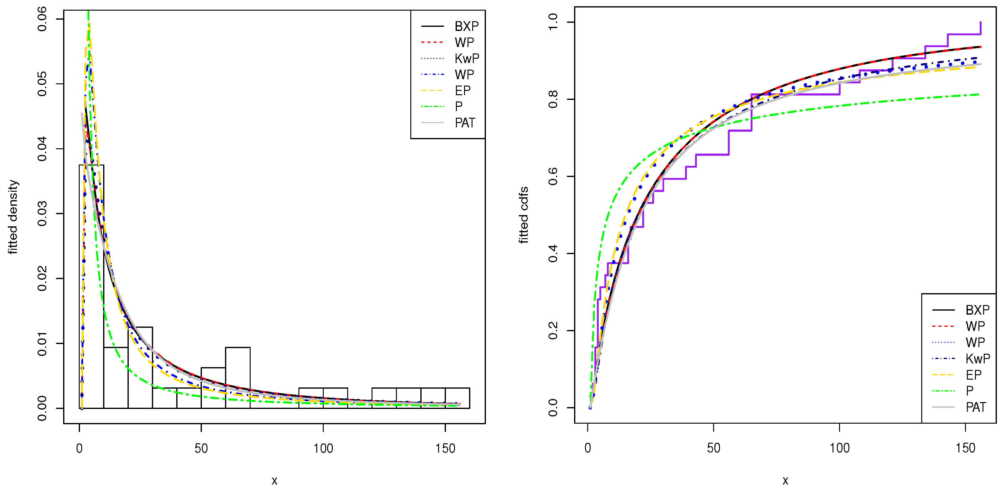
The first dataset gives the survival times, in weeks, of 33 patients suffering from acute myelogenous leukaemia. These data have been introduced by Feigl and Zelen (1965) and analysed by Mead et al. (2017). The data are: 65, 156, 100, 134, 16, 108, 121, 4, 39, 143, 56, 26, 22, 1, 1, 5, 65, 56, 65, 17, 7, 16, 22, 3, 4, 2, 3, 8, 4, 3, 30, 4, 43. This dataset is well known as being bathtub hrf-shaped.
The second data-set shows the time intervals of the successive earthquakes in the last century in the North Anatolia fault zone between to north latitude and to east longitude. This dataset was introduced and analysed by Kuş (2007). This dataset is well known as being decreasing hrf-shaped.
For both datasets, the estimated parameters based on the MLE method are given in Table 3, whereas the values of the information criteria and goodness-of-fit statistics are given in Table 4. Since MLE of the equals the minimum order statistics, we suppose it as known to be the minimum value the dataset. Table 4 shows that the BXP distribution has the lowest values of these statistics among all the fitted models. Hence, it could be chosen as the best model under these criteria for both datasets.
8. Value-at-Risk Estimation with the BXP Distribution
In this section, the performance of BXP distribution in estimating Value-at-Risk (VaR) is discussed and compared with the Generalized P (GP) distribution. GP is a widely-used distribution in actuarial sciences, economics and statistics to model the tail of the distribution that contains extreme events. VaR is one of the most popular approaches to measure market risk. From a statistical point of view, the VaR entails the estimation of the quantile of the distribution of returns. The VaR for a long position (left tail of the distribution function) over a given time horizon tis defined as:
where F is the distribution function of financial losses, denotes the inverse of F and p is the quantile at which VaR is calculated.
The Peaks-Over-Threshold (POT) method is used to model the tail of the distribution. POT is based on the distribution of exceedances over a given threshold. The conditional excess distribution, , can be defined as follows:
where random variable X represents the financial losses, u is the threshold, are the excesses and is the right endpoint of F. can be re-defined as follows:
The Balkema and De Haan (1974) and Pickands (1975) theorem shows that for a sufficiently high threshold u, the excess distribution function can be approximated by the GP distribution:
where for and for and and are shape and scale parameters of the GP distribution, respectively. Isolating from (14), we get:
where is the GP distribution and . Then, substituting (14) in (16), the following estimate for is obtained:
where and are maximum likelihood estimates of and , respectively. Inverting (17) for a given probability p, can be obtained as:
Threshold selection is a difficult task and an essential part for tail modelling with the GP distribution. The most used method is the Mean Excess (ME) plot for the determination of the threshold. The ME function can be defined as follows:
where I is the indicator function. When the empirical ME function is a positively sloped straight line above a certain threshold u, it is evidence that the used dataset follows the GP distribution with a positive parameter.
Here, the BXP distribution is adopted in the POT method. It is assumed that BXP provides a good approximation to for a sufficiently high threshold u. Then, substituting the cdf of BXP in (16), the new estimate for can be obtained as:
The can be obtained by inverting (20) for a given probability p, as follows:
where and are the maximum likelihood estimates of and , respectively.
8.1. S&P-500
To evaluate and compare the performance of the BXP with GP distribution in terms of VaR accuracy, the S&P-500 index is used. The used time series data contain 1465 daily log returns from 4 January 2012 to 27 October 2017. The descriptive statistics of S&P-500 are given in Table 4.
Table 5 shows that the mean returns are closed to zero. The Jarque–Bera statistics in Table 5 also show that the null hypothesis of normality is rejected at any level of significance, as evidenced by the high excess kurtosis and negative skewness. Thus, it is clear that log returns of S&P-500 indexes have non-normal characteristics, excess kurtosis and fat tails. The result of the Ljung–Box test indicates that the raw returns are free from autocorrelation. Therefore, BXP and GP distributions could be applied to the independent and identically distributed observations.
The ME plot is used to determine the optimal threshold value for the POT method. Figure 4 displays the ME plot of the S&P-500 dataset. The optimal threshold could be chosen as 0.02 for the used dataset. It is near the 90% quantile value of the S&P-500.
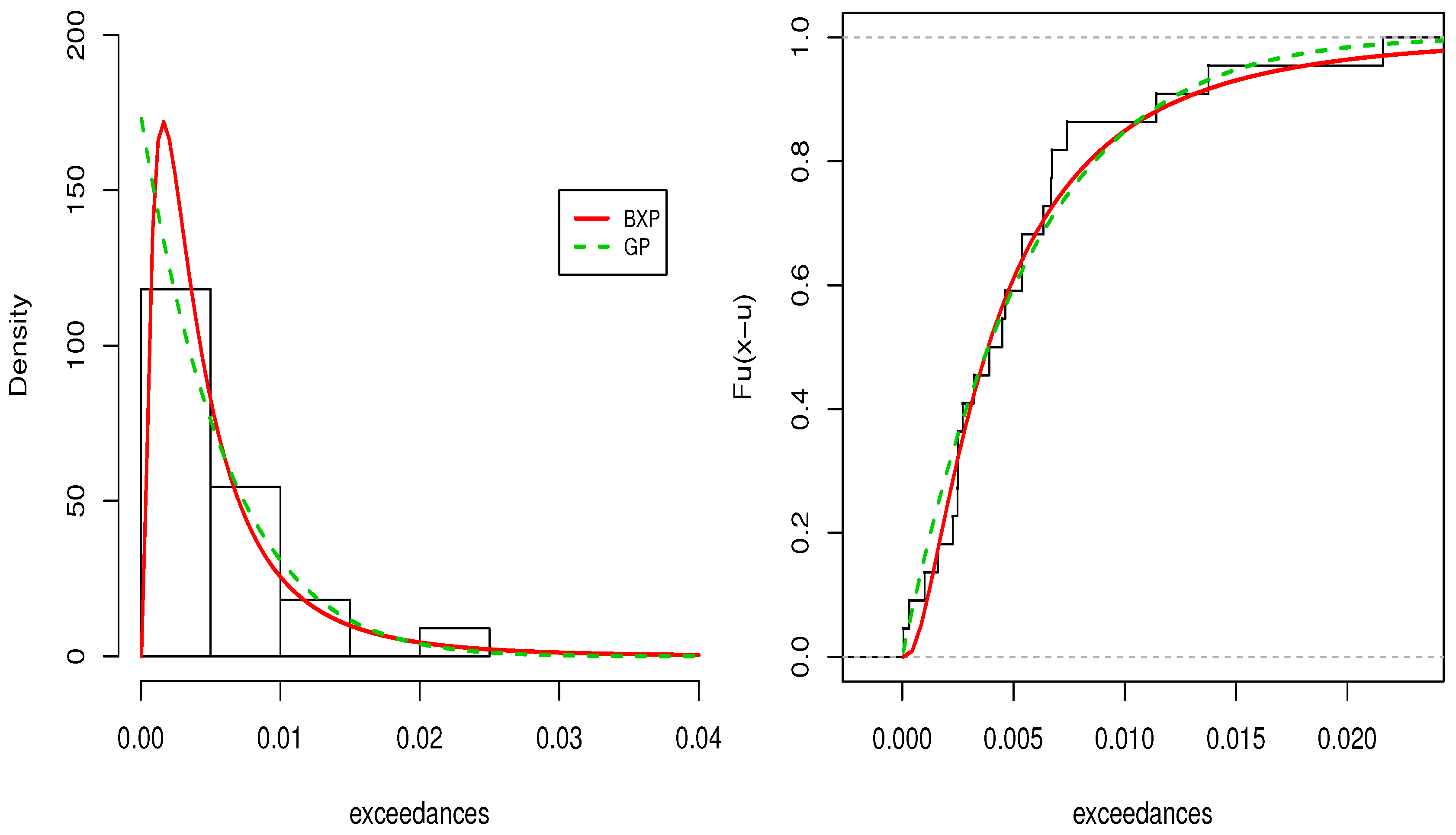
Table 6 shows the estimated parameters of BXP distribution and GP distribution using the POT method for the S&P-500 dataset. Based on the figures in Table 6, we conclude that since the BXP distribution has the lowest values of these statistics, BXP provides better fits than the GP distribution for tail modelling of S&P-500 indexes. Figure 5 displays the fitted pdf and cdfs of the BXP and GP distributions. Figure 5 reveals that the BXP distribution provides superior fits to the used dataset.
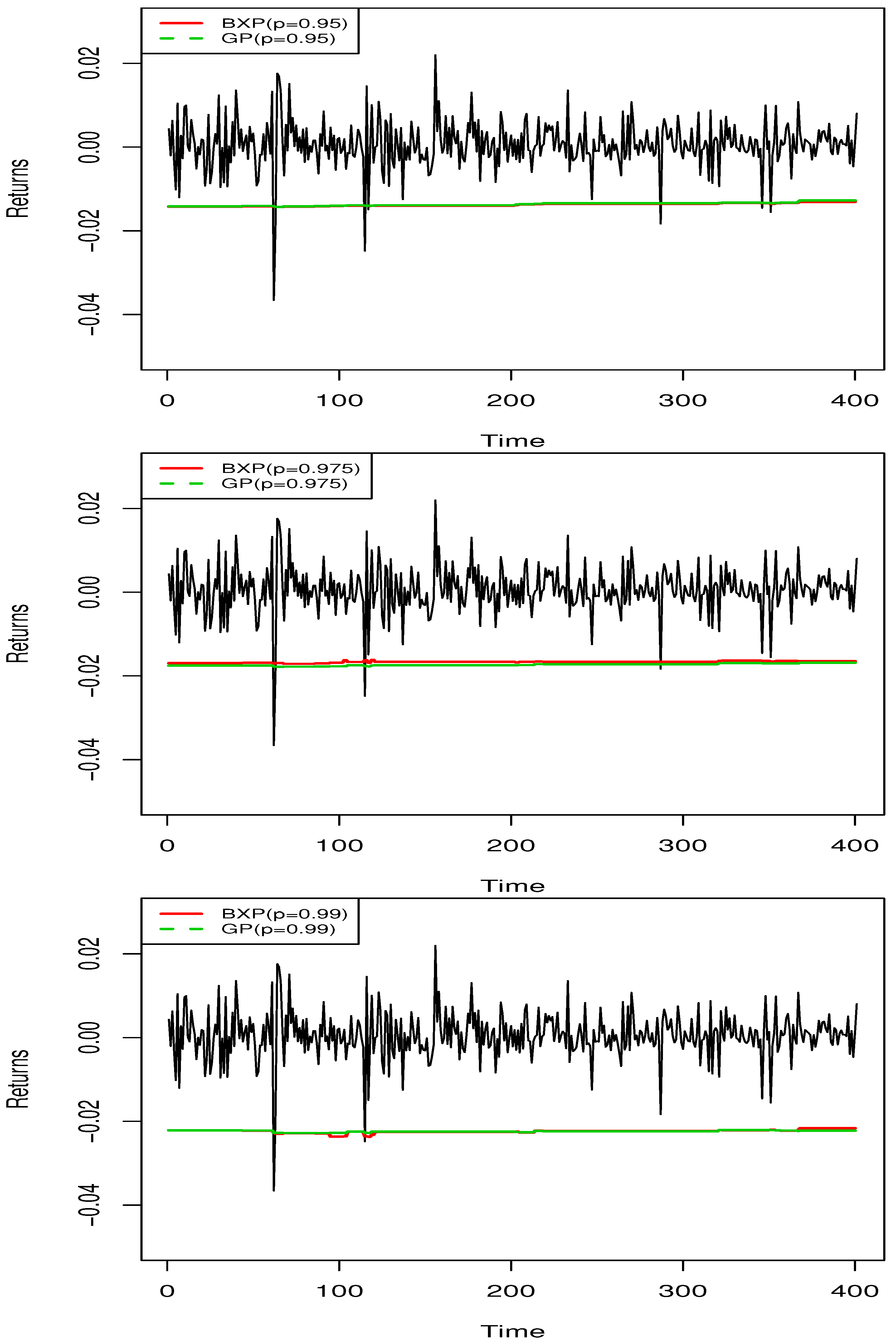
Here, VaR is estimated with the GP and BXP distribution using the POT method for values of and . The rolling window estimation method is used to evaluate the out-of-sample performance of the GP and BXP models. The first 1064 daily returns are used as the window length, and the next 400 data points are considered as out-of-sample period. Figure 6 displays daily VaR estimates of the BXP and GP models. Based on Figure 6, it is clear that the BXP and GP models produce similar VaR estimates. Therefore, the BXP model could be considered as an alternative VaR model against to GP model for financial institutions.
In VaR estimation, using the POT method is applied to raw return data assuming the distribution to be stationary or unconditional without considering the time-varying volatility. The POT method can also be considered as a dynamic model, where the conditional distribution of F is taken into account and the volatility of returns is captured. The dynamic POT method based on the BXP distribution, combined with the generalized autoregressive conditional heteroscedasticity type process, introduced by Bollerslev (1986), could be considered as future work of this study.
9. Conclusions
In this study, we proposed a new distribution that was referred to as the Burr X Pareto (BXP) using the Burr X generator. Some mathematical properties were obtained. The estimation of the model parameters is performed by the MLE, LS and WLS methods. We compare the distribution with a few other models using two real datasets. It is expected that the BXP distribution will serve as a better alternative in modelling real-life datasets. Value-at-Risk estimation with the BXP distribution is presented using time series data, we showed that the new model could be considered as an alternative VaR model against the generalized Pareto model for financial institutions.
Author Contributions
Mustafa Ç. Korkmaz, Emrah Altun, Haitham M. Yousof, Ahmed Z. Afify and Saralees Nadarajah have contributed jointly to all of the sections of the paper.
Conflicts of Interest
The authors declare no conflict of interest.
References
- Afify, Ahmed Z., Haitham M. Yousof, Gholamhossein Hamedani, and Gokarna Aryal. 2016. The exponentiated Weibull-Pareto distribution with Application. Journal of Statistical Theory and Applications 15: 326–44. [Google Scholar] [CrossRef]
- Akinsete, Alfred, Felix Famoye, and Carl Lee. 2008. The beta-Pareto distribution. Statistics 42: 547–63. [Google Scholar] [CrossRef]
- Balkema, August Aimé, and Laurens De Haan. 1974. Residual life time at great age. The Annals of Probability 2: 792–804. [Google Scholar] [CrossRef]
- Bourguignon, Marcelo, Rodrigo B. Silva, Luz M. Zea, and Gauss M. Cordeiro. 2013. The Kumaraswamy Pareto distribution. Journal of Statistical Theory and Applications 12: 129–44. [Google Scholar] [CrossRef]
- Bollerslev, Tim. 1986. Generalized autoregressive conditional heteroskedasticity. Journal of Econometrics 31: 307–27. [Google Scholar] [CrossRef]
- Feigl, Polly, and Marvin Zelen. 1965. Estimation of exponential survival probabilities with concomitant information. Biometrics 21: 826–38. [Google Scholar] [CrossRef] [PubMed]
- Gómez-Déniz, Emilio, and Enrique Calderín-Ojeda. 2015. Modelling insurance data with the Pareto ArcTan distribution. ASTIN Bulletin The Journal of the International Actuarial Association 45: 639–60. [Google Scholar] [CrossRef]
- Gupta, Ramesh C., Pushpa Gupta, and Rameshwar Gupta. 1998. Modeling failure time data by Lehmann alternatives. Communications in Statistics-Theory and Methods 27: 887–904. [Google Scholar] [CrossRef]
- Johnson, Norman L., Samuel Kotz, and Narayanaswamy Balakrishnan. 1994. Continuous Univariate Distributions. New York: Wiley, vol. 1. [Google Scholar]
- Kuş, Coşkun. 2007. A new lifetime distribution. Computational Statistics & Data Analysis 51: 4497–509. [Google Scholar]
- Mead, Mohamed E., Ahmed Z. Afify, Gholamhossein Hamedani, and Indranil Ghosh. 2017. The beta exponential Frechet distribution with applications. Austrian Journal of Statistics 46: 41–63. [Google Scholar] [CrossRef]
- Nadarajah, Saralees, and Sumaya Eljabri. 2013. The Kumaraswamy GP distribution. Journal of Data Science 11: 739–66. [Google Scholar]
- Pickands, James, III. 1975. Statistical inference using extreme order statistics. The Annals of Statistics 3: 119–31. [Google Scholar]
- Stoppa, Gabriele. 1990. A new model for income size distribution. In Income and Wealth Distribution, Inequality and Poverty. Berlin: Springer, pp. 33–41. [Google Scholar]
- Swain, James J., Sekhar Venkatraman, and James R. Wilson. 1988. Least squares estimation of distribution function in Johnsons translation system. Journal of Statistical Computation and Simulation 29: 271–97. [Google Scholar] [CrossRef]
- Tahir, Muhammad H., Gauss M. Cordeiro, Ayman Alzaatreh, M. Mansoor, and M. Zubair. 2016. A New Weibull-Pareto Distribution: Properties and Applications. Communications in Statistics-Simulation and Computation 45: 3548–67. [Google Scholar] [CrossRef]
- Yousof, Haitham M., Ahmed Z. Afify, Gholamhossein Hamedani, and Gokarna Aryal. 2016. The Burr X generator of distributions for lifetime data. Journal of Statistical Theory and Applications 16: 1–19. [Google Scholar] [CrossRef]
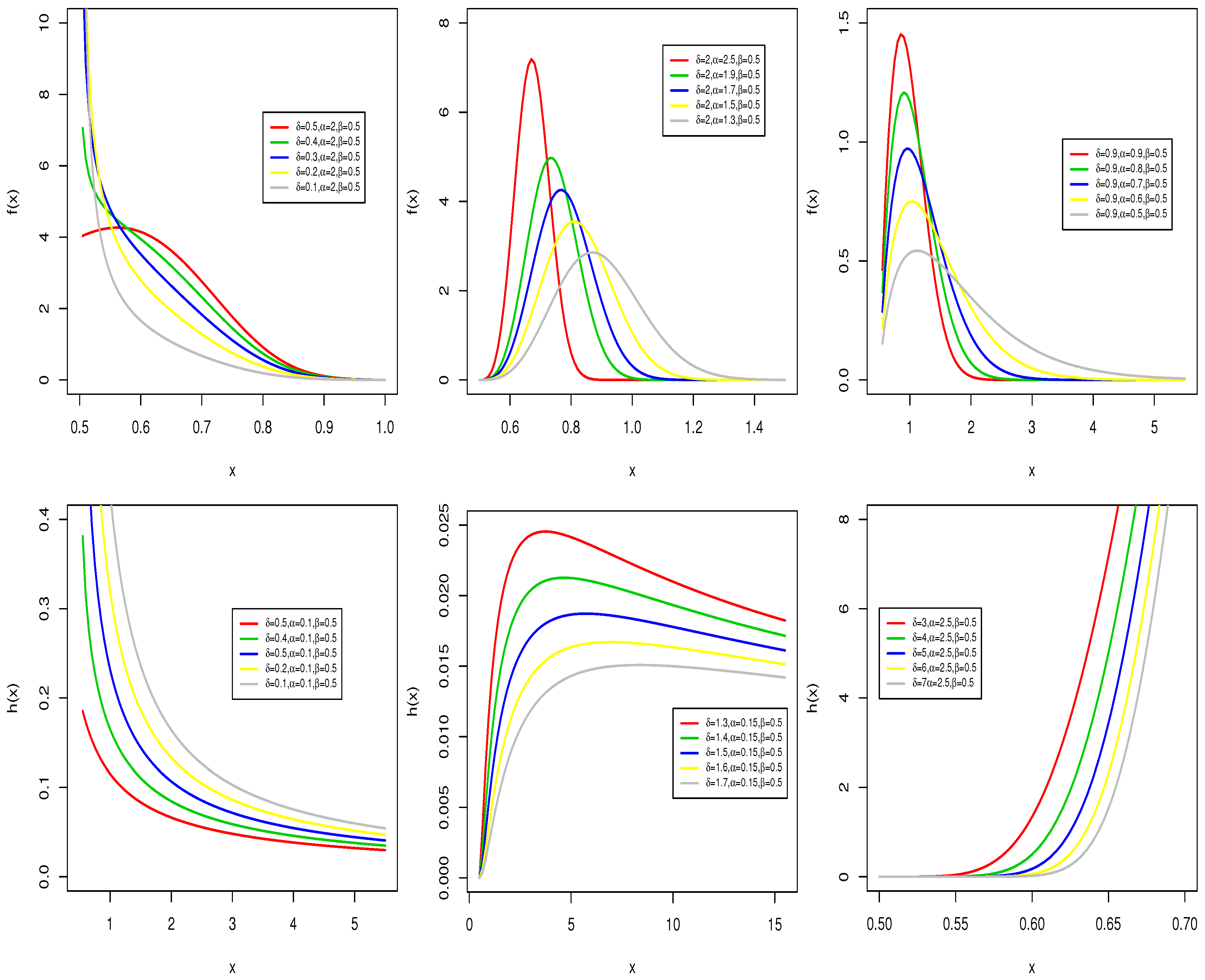
Figure 1.
Plots of the Burr XPareto (BXP) pdf (top) and plots of the BXP hazard rate function (hrf) (bottom).
Figure 1.
Plots of the Burr XPareto (BXP) pdf (top) and plots of the BXP hazard rate function (hrf) (bottom).

Figure 2.
Fitted pdfs (left panel) and cdfs (right panel) of leukaemia data.

Figure 3.
Fitted pdfs (left panel) and cdfs (right panel) of earthquake data.
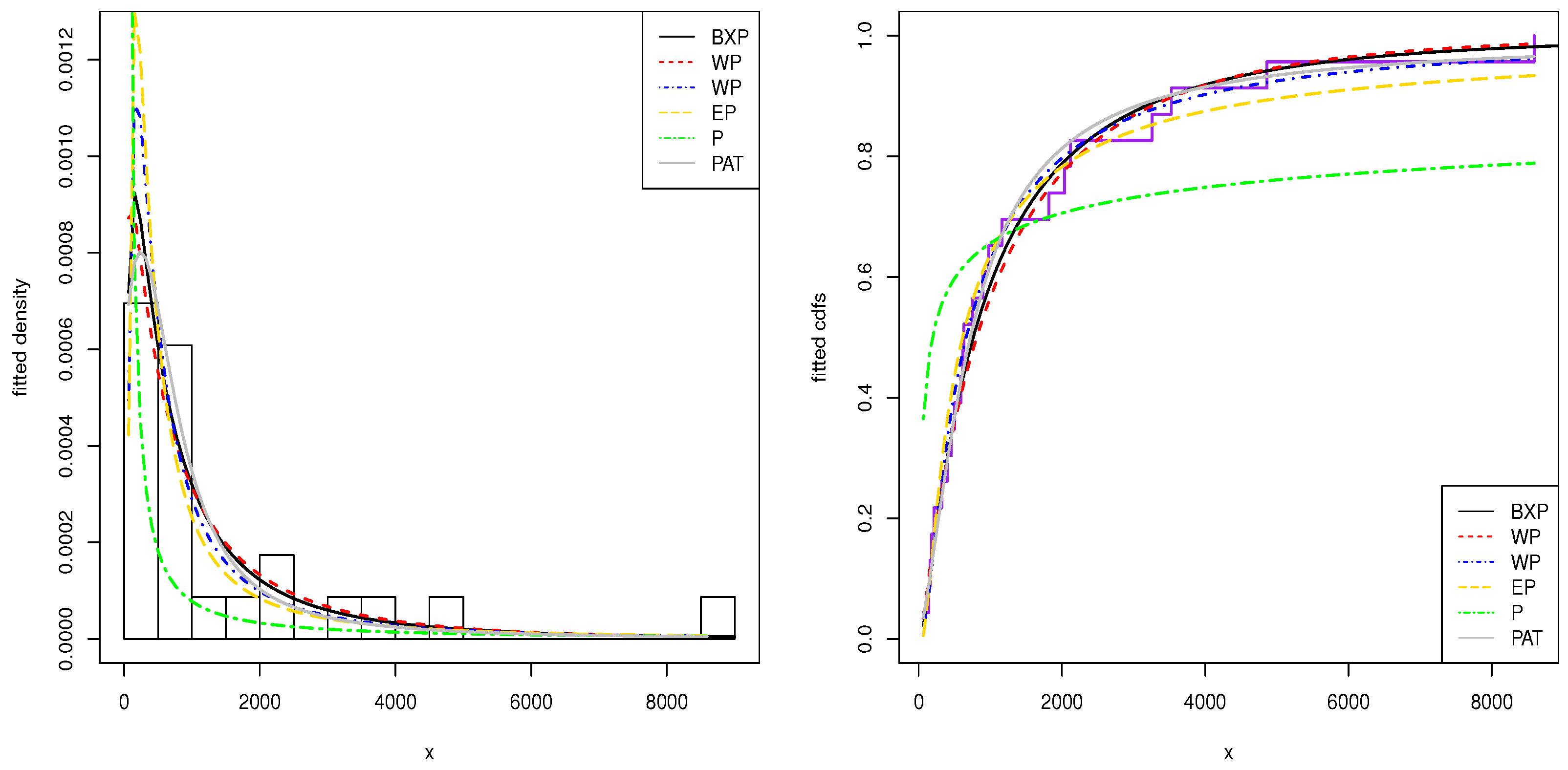
Figure 4.
Mean excess plot of the S&P-500 dataset.
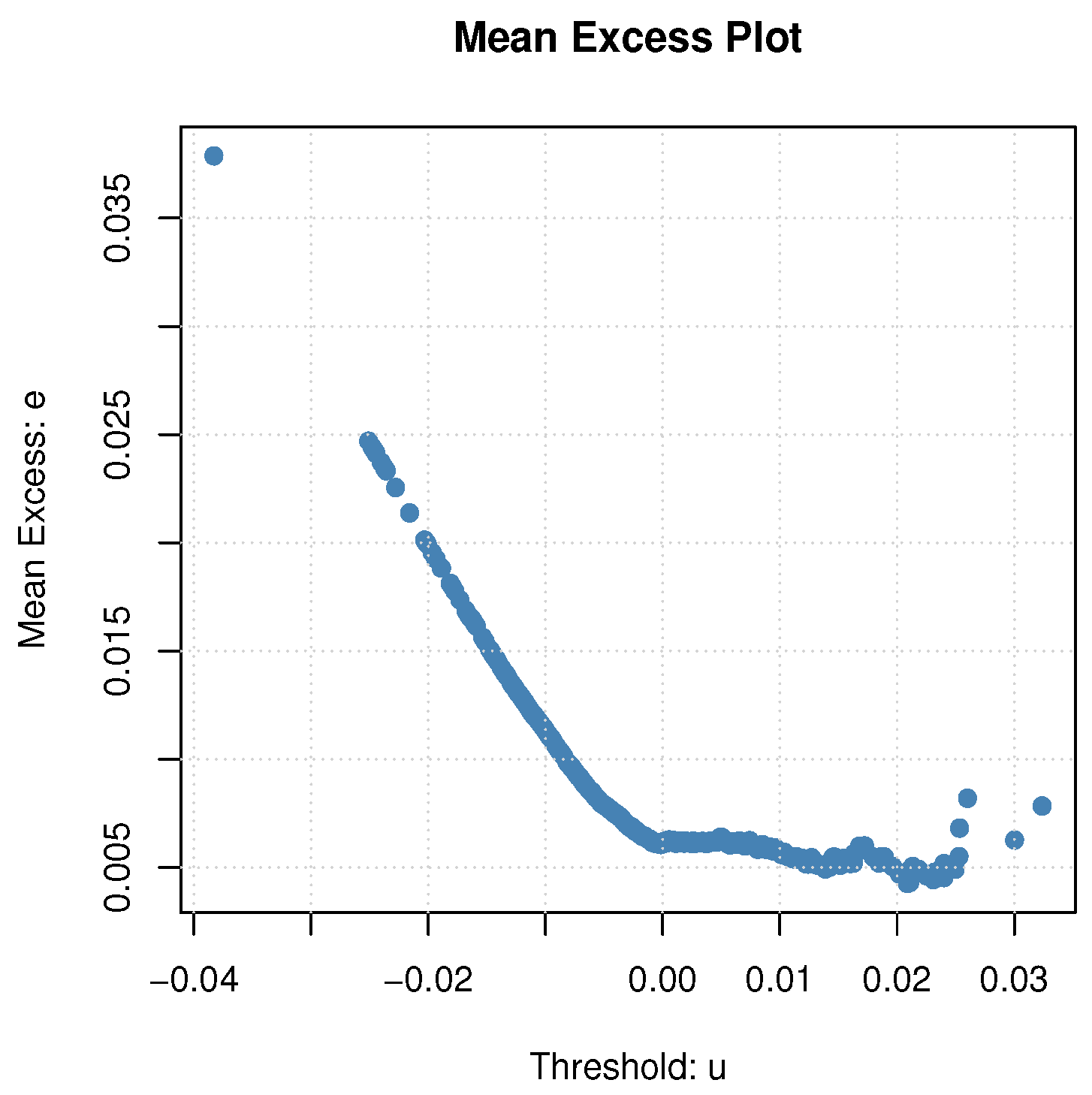
Figure 5.
Fitted pdfs (left) and cdfs (right) of the BXP and GP distribution for the S&P-500 dataset.
Figure 5.
Fitted pdfs (left) and cdfs (right) of the BXP and GP distribution for the S&P-500 dataset.

Figure 6.
Daily VaR estimates of the BXP and GP models.


Table 1.
Mean, variance, coefficients of skewness and kurtosis for different values of parameters.
| (0.5, 0.5, 0.5) | 1.2801 | 1.1395 | 0.7311 | 4.4238 |
| (1, 1, 1) | 1.6330 | 0.9671 | −1.2539 | 3.2132 |
| (2, 2, 2) | 2.5365 | 1.7311 | −1.9644 | 4.3986 |
| (1, 2, 3) | 2.9606 | 5.9323 | −0.8355 | 1.3785 |
| (4, 2, 0.5) | 0.7411 | 0.0415 | −4.1218 | 17.7934 |
| (10, 2, 0.25) | 0.4074 | 0.0011 | −6.3710 | 97.4674 |
| (0.25, 5, 2) | 0.4962 | 1.2671 | 1.4287 | 2.6058 |
| (0.9, 5, 1.8) | 1.0633 | 1.5440 | 0.0255 | 0.7191 |
Table 2.
The empirical means, sds (given in ), biases (given in ) and MSEs (given in ) for the special BXP distributions.
Table 2.
The empirical means, sds (given in ), biases (given in ) and MSEs (given in ) for the special BXP distributions.
| Parameters | |||||||||
|---|---|---|---|---|---|---|---|---|---|
| 3, 1.5, 2 | 3.0144 | 1.5495 | 2.0286 | 2.9995 | 1.5247 | 2.0159 | 3.0001 | 1.5125 | 2.0060 |
| (0.1831) | (0.1585) | (0.1155) | (0.0399) | (0.1059) | (0.0757) | (0.0400) | (0.0648) | (0.0485) | |
| [0.0144] | [0.0494] | [0.0286] | [−0.0005] | [0.0247] | [0.0160] | [0.0001] | [0.0125] | [0.0059] | |
| {0.0330} | {0.0270} | {0.0140} | {0.0016} | {0.0117} | {0.0060} | {0.0016} | {0.0043} | {0.0023} | |
| 3, 2, 1 | 3.0772 | 2.0550 | 1.0040 | 3.0019 | 2.0093 | 1.0021 | 3.0016 | 2.0073 | 1.0013 |
| (0.2928) | (0.2053) | (0.0443) | (0.0212) | (0.0976) | (0.0211) | (0.0203) | (0.0851) | (0.0182) | |
| [0.0772] | [0.0550] | [0.0040] | [0.0019] | [0.0093] | [0.0021] | [0.0016] | [0.0073] | [0.0013] | |
| {0.0900} | {0.0443} | {0.0020} | {0.0004} | {0.0095} | {0.0004} | {0.0004} | {0.0072} | {0.0003} | |
| 5, 0.5, 5 | 5.0863 | 0.5111 | 5.1216 | 5.0044 | 0.5012 | 5.0065 | 4.9954 | 0.4996 | 4.9970 |
| (0.2792) | (0.0290) | (0.3641) | (0.0404) | (0.0095) | (0.0490) | (0.0400) | (0.0084) | (0.0439) | |
| [0.0863] | [0.0111] | [0.1216] | [0.0044] | [0.0012] | [0.0065] | [−0.0046] | [−0.0004] | [−0.0030] | |
| {0.0838} | {0.0010} | {0.1447} | {0.0072} | {0.00008} | {0.0071} | {0.0054} | {0.00007} | {0.0070} | |
| 10, 30, 20 | 10.0407 | 30.0438 | 20.0024 | 10.0009 | 30.0013 | 19.9998 | 9.9984 | 29.9980 | 20.0001 |
| (0.2318) | (0.2809) | (0.0101) | (0.0110) | (0.0130) | (0.0086) | (0.0101) | (0.0120) | (0.0059) | |
| [0.0406] | [0.0438] | [0.0024] | [0.0009] | [0.0013] | [−0.0002] | [−0.0016] | [−0.0020] | [0.0001] | |
| {0.0543} | {0.0793} | {0.0001} | {0.0001} | {0.0001} | {0.00007} | {0.0001} | {0.0001} | {0.00004} | |
| 4, 0.5, 0.5 | 3.9077 | 0.5147 | 0.5265 | 4.0179 | 0.5121 | 0.5203 | 4.0012 | 0.5052 | 0.5079 |
| (0.1261) | (0.0532) | (0.0926) | (0.1010) | (0.0411) | (0.0711) | (0.0878) | (0.0246) | (0.0440) | |
| [−0.0923] | [0.0147] | [0.0265] | [0.0179] | [0.0121] | [0.0203] | [0.0012] | [0.0052] | [0.0079] | |
| {0.0356} | {0.0030} | {0.0100} | {0.0164} | {0.0018} | {0.0054} | {0.0076} | {0.0006} | {0.0019} | |
Table 3.
MLEs and their standard errors (in parentheses) for both datasets. P, Pareto; PAT, P ArcTan; KwP, Kumaraswamy P; WP, Weibull P; BP, Beta P; EP, Exponentiated P.
Table 3.
MLEs and their standard errors (in parentheses) for both datasets. P, Pareto; PAT, P ArcTan; KwP, Kumaraswamy P; WP, Weibull P; BP, Beta P; EP, Exponentiated P.
| Leukaemia Data | ||||
| Model | ||||
| BXP | 0.8505 | 0.1900 | 1 | |
| (0.1785) | (0.0146) | |||
| PAT | 0.8603 | 12.6124 | 1 | |
| (0.1428) | (6.6619) | |||
| KwP | 2.3992 | 0.0007 | 1,828,015 | 1 |
| (0.0291) | (0.0001) | (5.9317) | ||
| WP | 1.8274 | 0.1994 | 1 | |
| (0.2846) | (0.0145) | |||
| BP | 51.9800 | 0.0239 | 3.8540 | 1 |
| (0.1240) | (0.0048) | (0.6551) | ||
| EP | 4.3606 | 0.7089 | 1 | |
| (1.3221) | (0.1192) | |||
| P | 0.3319 | 1 | ||
| (0.0596) | ||||
| Earthquake Data | ||||
| BXP | 1.9916 | 0.1678 | 9 | |
| (0.5622) | (0.0117) | |||
| PAT | 1.1704 | 168.1574 | 9 | |
| (0.0667) | (5.9619) | |||
| WP | 2.9843 | 0.1408 | 9 | |
| (0.4949) | (0.0074) | |||
| BP | 60.8341 | 0.0428 | 12.5592 | 9 |
| (1.0981) | (0.0053) | (0.9570) | ||
| EP | 26.9837 | 0.8707 | 9 | |
| (5.7196) | (0.0770) | |||
| P | 0.2264 | 9 | ||
| (0.0472) | ||||
Table 4.
Goodness-of-fit statistics for both datasets. CAIC, Corrected Akaike Information Criterion; HQIC, Hannan–Quinn Information Criterion.
Table 4.
Goodness-of-fit statistics for both datasets. CAIC, Corrected Akaike Information Criterion; HQIC, Hannan–Quinn Information Criterion.
| Leukaemia Data | |||||
|---|---|---|---|---|---|
| Model | AIC | CAIC | BIC | HQIC | KS |
| BXP | 295.0115 | 295.4401 | 297.8795 | 295.9464 | 0.1328 |
| PAT | 301.1477 | 301.5763 | 304.0157 | 302.0826 | 0.1398 |
| KwP | 298.9148 | 299.8037 | 303.2167 | 300.3171 | 0.1486 |
| WP | 295.2830 | 295.7116 | 298.1510 | 296.2179 | 0.1418 |
| BP | 301.5970 | 302.4859 | 305.8990 | 302.9994 | 0.1494 |
| EP | 300.9643 | 301.3929 | 303.8323 | 301.8992 | 0.1630 |
| P | 319.1294 | 319.2673 | 320.5634 | 319.5968 | 0.2733 |
| Earthquake Data | |||||
| BXP | 381.9004 | 382.5004 | 384.1714 | 382.4715 | 0.0817 |
| PAT | 383.7187 | 384.3187 | 385.9897 | 384.2899 | 0.0971 |
| WP | 382.3901 | 382.9901 | 384.6610 | 382.9612 | 0.0962 |
| BP | 384.5029 | 385.7661 | 387.9094 | 385.3597 | 0.0819 |
| EP | 384.3233 | 384.9233 | 386.5943 | 384.8944 | 0.1038 |
| P | 420.6338 | 420.8243 | 421.7693 | 420.9194 | 0.4218 |
Table 5.
Summary statistics for the S&P-500 index.
| Descriptive Statistics | S&P-500 |
|---|---|
| Number of observations | 1465 |
| Minimum | −0.0402 |
| Maximum | 0.0383 |
| Mean | 0.0004 |
| Median | 0.0004 |
| Std.Deviation | 0.007 |
| Skewness | −0.322 |
| Kurtosis | 5.403 |
| Jarque–Bera | 377.839 (<0.001) |
| Ljung–Box | 28.516 (0.098) |
Table 6.
MLEs, corresponding standard errors (in second line) and goodness-of-fit statistics for the S&P-500.
Table 6.
MLEs, corresponding standard errors (in second line) and goodness-of-fit statistics for the S&P-500.
| Models | Parameters | Goodness-of-Fit | |||||||
|---|---|---|---|---|---|---|---|---|---|
| KS | |||||||||
| BXP | 3.2480 | 0.1893 | 4.89818 × 10 | −93.4016 | 0.1427 | 0.3809 | 0.0556 | ||
| 1.0266 | 0.0120 | - | |||||||
| GP | 0.0847 | 0.0057 | −88.7171 | 0.1498 | 0.4039 | 0.0661 | |||
| 0.1996 | 0.0015 | ||||||||
© 2017 by the authors. Licensee MDPI, Basel, Switzerland. This article is an open access article distributed under the terms and conditions of the Creative Commons Attribution (CC BY) license (http://creativecommons.org/licenses/by/4.0/).
Share and Cite
MDPI and ACS Style
Korkmaz, M.Ç.; Altun, E.; Yousof, H.M.; Afify, A.Z.; Nadarajah, S. The Burr X Pareto Distribution: Properties, Applications and VaR Estimation. J. Risk Financial Manag. 2018, 11, 1. https://doi.org/10.3390/jrfm11010001
AMA Style
Korkmaz MÇ, Altun E, Yousof HM, Afify AZ, Nadarajah S. The Burr X Pareto Distribution: Properties, Applications and VaR Estimation. Journal of Risk and Financial Management. 2018; 11(1):1. https://doi.org/10.3390/jrfm11010001
Chicago/Turabian StyleKorkmaz, Mustafa Ç., Emrah Altun, Haitham M. Yousof, Ahmed Z. Afify, and Saralees Nadarajah. 2018. "The Burr X Pareto Distribution: Properties, Applications and VaR Estimation" Journal of Risk and Financial Management 11, no. 1: 1. https://doi.org/10.3390/jrfm11010001