Investigation of the Financial Stability of S&P 500 Using Realized Volatility and Stock Returns Distribution


Faculty of Engineering and Technology, Department of Computer Science and Telecommunication Engineering, Noakhali Science and Technology University, Noakhali 3814, Bangladesh
*
Authors to whom correspondence should be addressed.
J. Risk Financial Manag. 2018, 11(2), 22; https://doi.org/10.3390/jrfm11020022
Submission received: 2 April 2018
/
Revised: 20 April 2018
/
Accepted: 26 April 2018
/
Published: 28 April 2018
(This article belongs to the Special Issue Stock Market Volatility Modelling and Forecasting)
Abstract
:In this work, the financial data of 377 stocks of Standard & Poor’s 500 Index (S&P 500) from the years 1998–2012 with a 250-day time window were investigated by measuring realized stock returns and realized volatility. We examined the normal distribution and frequency distribution for both daily stock returns and volatility. We also determined the beta-coefficient and correlation among the stocks for 15 years and found that, during the crisis period, the beta-coefficient between the market index and stock’s prices and correlation among stock’s prices increased remarkably and decreased during the non-crisis period. We compared the stock volatility and stock returns for specific time periods i.e., non-crisis, before crisis and during crisis year in detail and found that the distribution behaviors of stock return prices has a better long-term effect that allows predictions of near-future market behavior than realized volatility of stock returns. Our detailed statistical analysis provides a valuable guideline for both researchers and market participants because it provides a significantly clearer comparison of the strengths and weaknesses of the two methods.

1. Introduction
At present, stock market investment is one of the most significant parts of the nations’ economy. It plays a vital role in leading the distributed liquidity and savings towards optimal paths to make sure that scarce financial resources are effectively allocated to the most profitable activities and projects (Zahedi and Rounaghi 2015; Nasrollahi 1992). The majority of capital is exchanged by stock markets throughout the world. Therefore, stock market performance can directly influence the national economy. If people have proper business insight, they can easily get a forecast about the stock market due to its macro and microeconomic activity. Stock market prediction that specifically deals with financial issues and stock market exchanges can be deemed as a necessity. In addition, the stock market can be affected by thousands of other factors with macro-parameters (Zahedi and Rounaghi 2015). People who would like to invest in common stock need to fix the share real value and then compare it with current market price. Therefore, in the stock market the most crucial part is predicting the stock price of listed companies and their estimated real value, since prices are a crucial point to guide the effective allocation of capital and liquidity that might be considered as a powerful tool in the efficient allocation of resources (Azizian 2006).
There lies a long history behind predicting stock returns in finance (Zahedi and Rounaghi 2015). This is unsurprising because the characterization of stock return predictability is the most crucial part for making portfolio allocation decisions and for fruitful understanding of the risk–return trade-off and market inefficiency. To date, predicting excess returns has produced a lot of literature that includes financial variables e.g., nominal interest rates, dividend:price ratios, term and default spreads, and a wide range of other markers (Azizian 2006). Though there might have been some controversy in predicting stock returns due to false regressions, data mining, and instability of return predictability, the literature always suggests that stock returns have a predictable component (Ang and Bekaert 2007; Campbell and Thompson 2008; Cochrane 2008; Pástor and Stambaugh 2009; Van Binsbergen and Koijen 2010). By considering stock return as a time series, most of the forecasting methods use statistical models to find out the hidden properties in the sequence, such as dependency and data distribution. Suggested statistical models are AR process (Summers 1996), Markov process and the artificial neural network (MPANN) model, auto-regression moving average (ARMA) (Constantinou et al. 2006), and generalized auto-regression conditional heteroscedasticity (GARCH) model (Huang 2009; Drakos et al. 2010). The empirical results specified that nonlinear models follow linear models (Matías and Reboredo 2012). Financial analysts are generally regarded as an important information source for stock investors as they can effectively process all kinds of information related to stock market (Sonney 2009).
On the other hand, many researchers suggest that stock return volatility is strongly related to market uncertainty and it is the key input in many investment decisions and in overall portfolio management. Studies have shown that volatility is the primary risk indicator and a reliable forecast of market volatility is pivotal (Green and Figlewski 1999). In terms of finance, volatility (σ) indicates the degree of variation over a period of a trading price that can be determined by the standard deviation of logarithmic returns (Glosten et al. 1993). A higher volatility means a dramatical change of security value over a short time period. When volatility increases, risk increases and returns decrease. A lower volatility means that a security’s value does not fluctuate dramatically, but changes in value at a steady bound over a period of time (Glosten et al. 1993). Crestmont Research showed the historical relationship between stock market performance and market volatility (Ang and Liu 2007). For this investigation, the average range for each day was used to measure the volatility of Standard & Poor’s 500 Index (S&P 500 index). This study proposed that higher volatility corresponds to a higher probability of a declining market whereas lower volatility represents higher probability of a rising market (Ang and Liu 2007). Glosten et al. (1993) investigated how volatility affects the risk premium of stocks and specified an adjusted GARCH-M model (Ang and Liu 2007).
Ang and Liu (2007) described the relationship between expected returns, risk, and dividends (Anderson 2000). The most important conclusions of this research are that there exists a positive relationship between high-dividend yield and high expected returns. Furthermore, there is a negative relationship between the risk premium and volatility, just like Glosten et al. (1993) found.
In this work, we compared the two most popular market predictability indicators—stock returns and volatilities—with distribution function for three separate years. We also determined how stock prices behave or move together in crisis and non-crisis periods. We calculated the cross-correlation and beta-coefficient for both the average realized returns and average absolute return and tried to find any difference between real or absolute price returns. Finally, we tried to investigate the distribution analysis with the real returns of the stock prices and also to find which distribution is better for forecasting an upcoming crisis period.
2. Materials and Methods
2.1. Data
We investigated the financial data of 377 stocks of Standard & Poor’s 500 Index for 15 years. We collected the data from Yahoo Finance. We also collected the S&P 500 historical index prices for the same years. The period of the data is from 1998 to 2012 where every year consists of 250 days.
2.2. Logarithmic Return
To investigate the relationship among the stocks and analyze the crisis period through correlation, covariance and two distributions while comparing between absolute and real stock returns, first we need to calculate the daily return. We calculated the real returns of the stock price of each company as:
And absolute return as
where Pi(t) is the daily closing price of stock i at day t.
For covariance and correlation calculation we will use both absolute and real returns.
2.3. Realized Volatility
In terms of finance, volatility (σ) indicates the degree of variation over a period of a trading price. It can be determined by standard deviation of logarithmic returns. We calculated the real volatility from the real logarithmic returns of the daily prices. The equation is as follows:
Here ; m = Average of all returns; n = Number of data points (returns).
2.4. Beta Coefficient
Beta coefficient is the measurement of sensitivity of a share price towards the market price. It can measure systematic risk, which indicates the risk inherent in the whole financial system. It can be determined from the slope of the security market line.
A beta coefficient of 1 denotes the risk carried by stock as the overall market. A coefficient below 1 indicates lower overall market risk and return while a coefficient higher than 1 suggests higher overall market risk and return.
2.5. Raw Stock Correlations
Beta-coefficient expresses the movement of stock prices with overall market prices. In addition, with beta-coefficient, correlation is necessary to determine the strength of the relationship. Pearson’s correlation coefficient (C(i,j) between every pair of stocks i and j) is used to calculate raw stock correlations, where
< > denotes average, and are the standard deviations (STD).
2.6. Descriptive Statistics
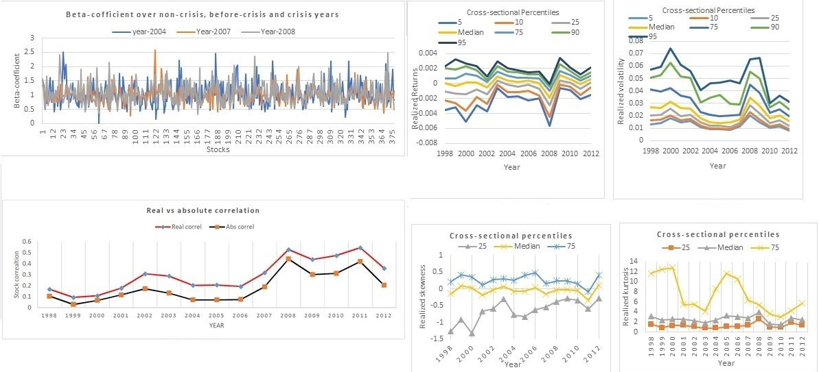
We calculated the frequency and normal distribution with descriptive statistics for raw stock realized return, realized volatility, realized skewness and realized kurtosis which shows calculation into 3 general classes, namely: location statistics (e.g., mean, median, mode, percentile), dispersion statistics (e.g., variance, standard deviation, range, interquartile range), and shape statistics (e.g., skewness, kurtosis). We plotted histogram, bell curve and cross-sectional percentiles from the descriptive statistics to show the behavior of frequency of stock returns, volatility, skewness and kurtosis during the crisis and non-crisis period.
2.7. Results and Discussion
Here the daily closing prices of 377 stocks from the S&P 500 from 1998 to 2012 were analyzed. These 377 stocks survived in the market during these periods. 250 days are considered for 1 year. Hence, we analyzed the market for total 15 years. In these periods, the market has been affected by different kinds of crisis e.g., Russian crisis in 1998, downturn of stock prices in 2002 due to the dot-com bubble, the September 11 attacks in 2001, the sub-prime mortgage crisis in 2007, the global financial crisis in 2008, and the European sovereign debt crisis in 2011 that modified the financial network hierarchy (Nobi and Lee 2017).
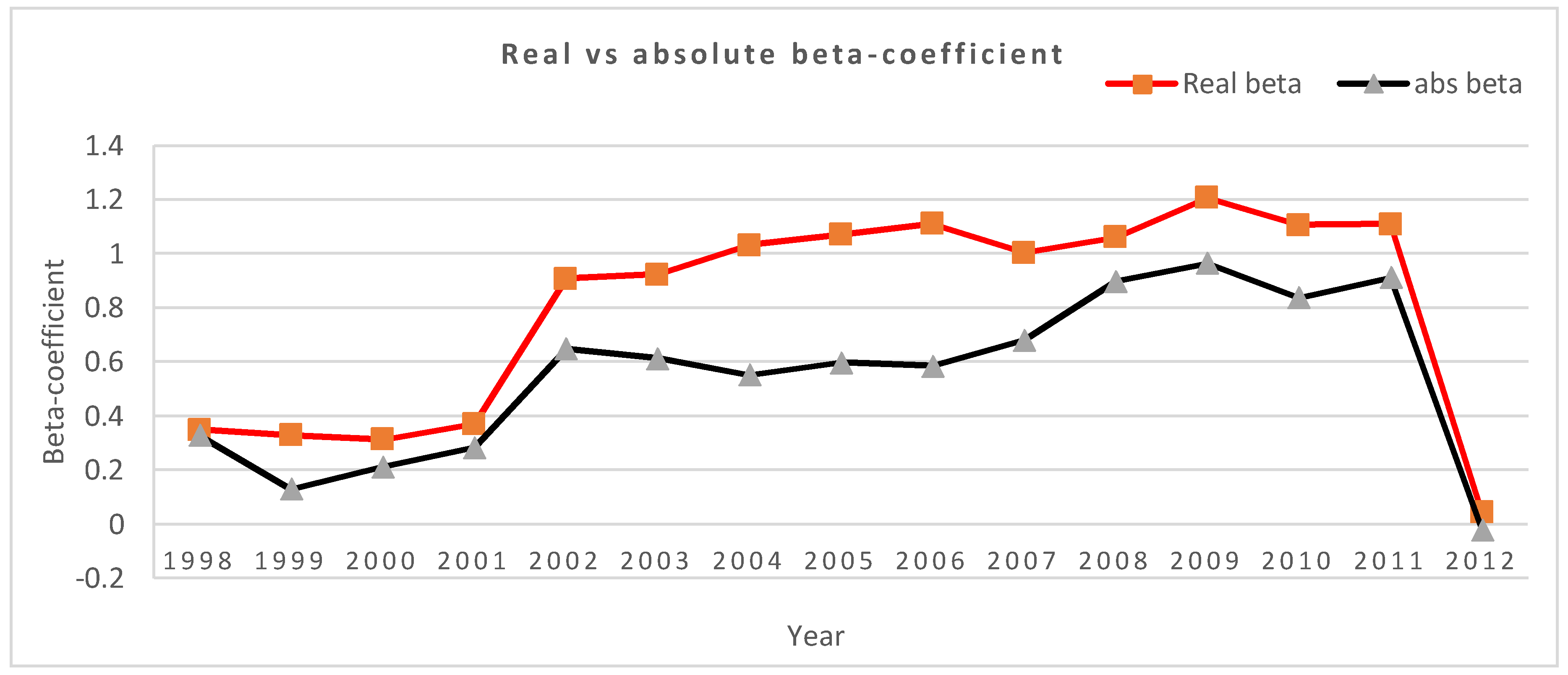
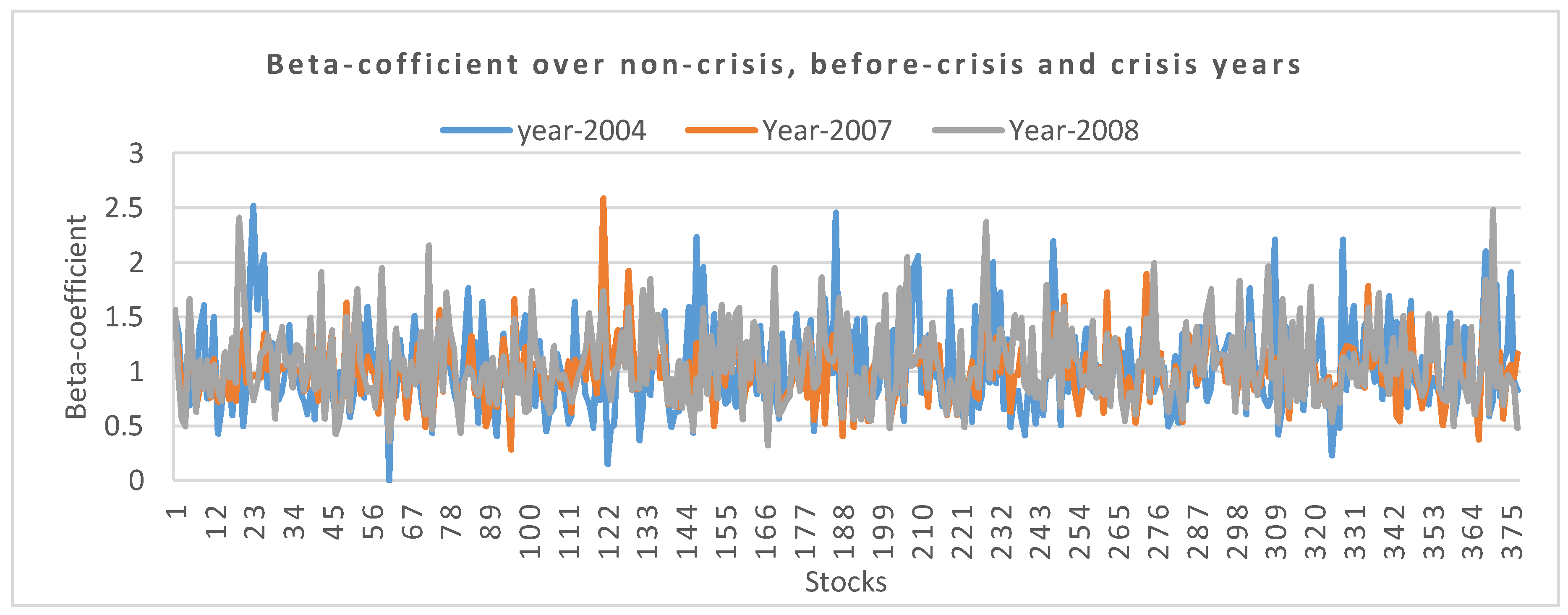
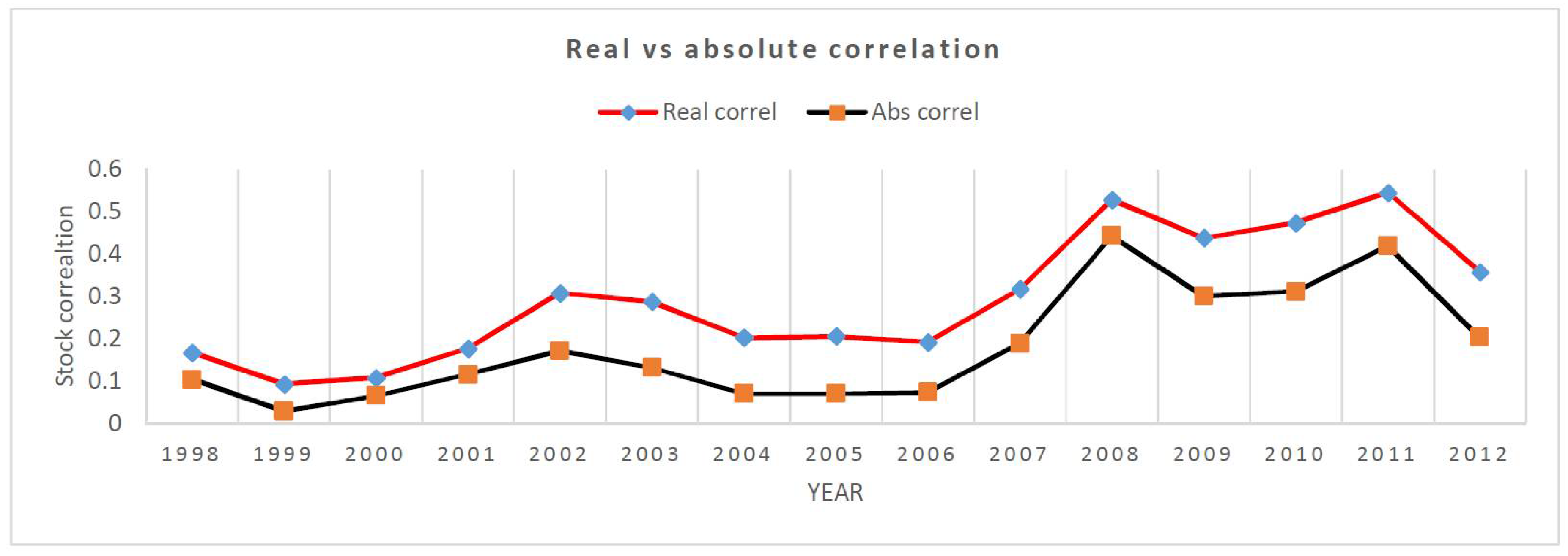
First, we calculated the average beta-coefficient for realized and absolute stocks returns in Figure 1 and then finalized the beta-behavior for three years i.e., non-crisis, before crisis and during-crisis periods in Figure 2. After that we calculated average cross-correlation for both realized and absolute return of the stocks for 15 years and observed that the two graphs in Figure 1 and Figure 3 shows approximately the same behavior for absolute returns during the periods. In Figure 1 it shows how the stocks are moved in relation to the market index over 15 years. In this case, the absolute beta-coefficient shows the significant identification of crisis periods rather than realized beta-coefficient. In addition, in some cases, the realized beta is misleading between crisis and non-crisis for the years 2003 to 2006. However, in the absolute beta result between the stock’s return and market index return, it is easily identified that in the non-crisis periods (1999, 2003–2006) the beta-coefficients of the stocks are very low in comparison with crisis periods (1998, 2000–2002, 2007–2009, 2011 etc.). The beta-coefficient between the stocks and market index increases during the crisis periods. Significantly, it is also found in Figure 2 that during the crisis periods, maximum stocks were showing similarity with market index and they became scattered or there was a very up-down relationship between stocks with market index during the non-crisis periods. Figure 2 shows the beta-behavior for non-crisis, before crisis and during-crisis periods. Figure 3 also clearly indicates that there is a positive relationship between beta and correlation in the stock market.
We also draw a correlation graph in Figure 3 among the stocks from the cross-correlation matrix which represents the correlation between returns for each stock. Here we also observed that the relationship between the stocks is increasing during the crisis period, i.e., the stock prices come closer and less scattered during the non-crisis period. After the crisis period 2011, in 2012 the correlation decreased, which implies that the market is going to recover. In addition, in this case the realized and absolute returns correlation shows the same behavior though realized returns has higher fluctuation than absolute returns.
Similar findings were reported for international stock-oil markets (Batten et al. 2018). They reported three time variables to denote the period from January 1990 to August 1997 (Asian Crisis in July 1997); August 1997 to October 2001 (effect of 11 September 2001); November 2001 until September 2008, (Lehman default on 15 September 2008). In each time variable, correlation increased during the crisis period and vice-versa (Batten et al. 2018). However, the lack of inter-industry correlation between the R2s of large firms and the R2s of size and industry-matched portfolios of smaller firms recommends that the explanatory power of universal factors may be same from one industry to another (Roll 1988).
Since we know the absolute returns results in a non-negative value, it will always exhibit positive skewness in distribution graph and hence we cannot predict the risks of stock market efficiently. Therefore, we computed our descriptive statistics with only realized stock price returns. We analyzed the mean, median, skewness, kurtosis, and percentile for both of volatility and stock returns. We tried to summarize the comparison between real stock returns and real volatility and further we investigated the stock returns realized skewness and realized kurtosis in both frequency distribution and cross-sectional percentile to monitor whether they have any relationship with stock returns and volatility or not. The Table 1 represents the total distribution comparison with realized returns, realized volatility, realized skewness, and realized kurtosis for the year 2004, 2007 and 2008.
For a clear and deep understanding of how the frequencies of stock returns and volatility moves during the non-crisis, crisis and before the crisis, we have only exhibited the results of the years 2004, 2008 and 2007.
From financial analysis, we know that the mean of stock returns has a great significance in market predictability: the lower the value of means, the higher the profit. In the case of stock returns the mean is very low in the year 2008 and negative, so it cannot be a good predictor of market stability. However, in volatility, the mean is high during the global financial crisis 2008. So, we can say high volatility is a risk indicator for the financial market. From Figure 4a in the non-crisis period 2004, the normal curve of returns is symmetrically distributed and the tails are positively skewed and in Figure 4b the frequency is only positively distributed in a discrete manner. The kurtosis of volatility is higher than the stock returns.
Before the crisis period in Figure 4c the stock returns are negatively skewed i.e., −0.766, but the volatility in Figure 4d is positively skewed. From stock returns distribution we can clearly predict that there may be a crisis in the future in the stock market. In addition, in Figure 4e it is more evident that the skewness has shifted into a more negative value and from Table 1 we can see it is −1.618. So, there is linear decrement in skewness in real stock returns. In addition, for real volatility, the skewness did not show any linear decrement or increment from crisis to non-crisis period. During the non-crisis period it was 1.760, before crisis 2.518 and during crisis 1.499. We can see the same characteristics on the kurtosis behavior of volatility distribution and a linear increment kurtosis from non-crisis to crisis period in stock return distribution. If we follow the volatility graph in Figure 4d we could not say that there is any probability of the market devastation which actually occurred in 2008, but from Figure 4c, a future crisis in 2008 can be forewarned.
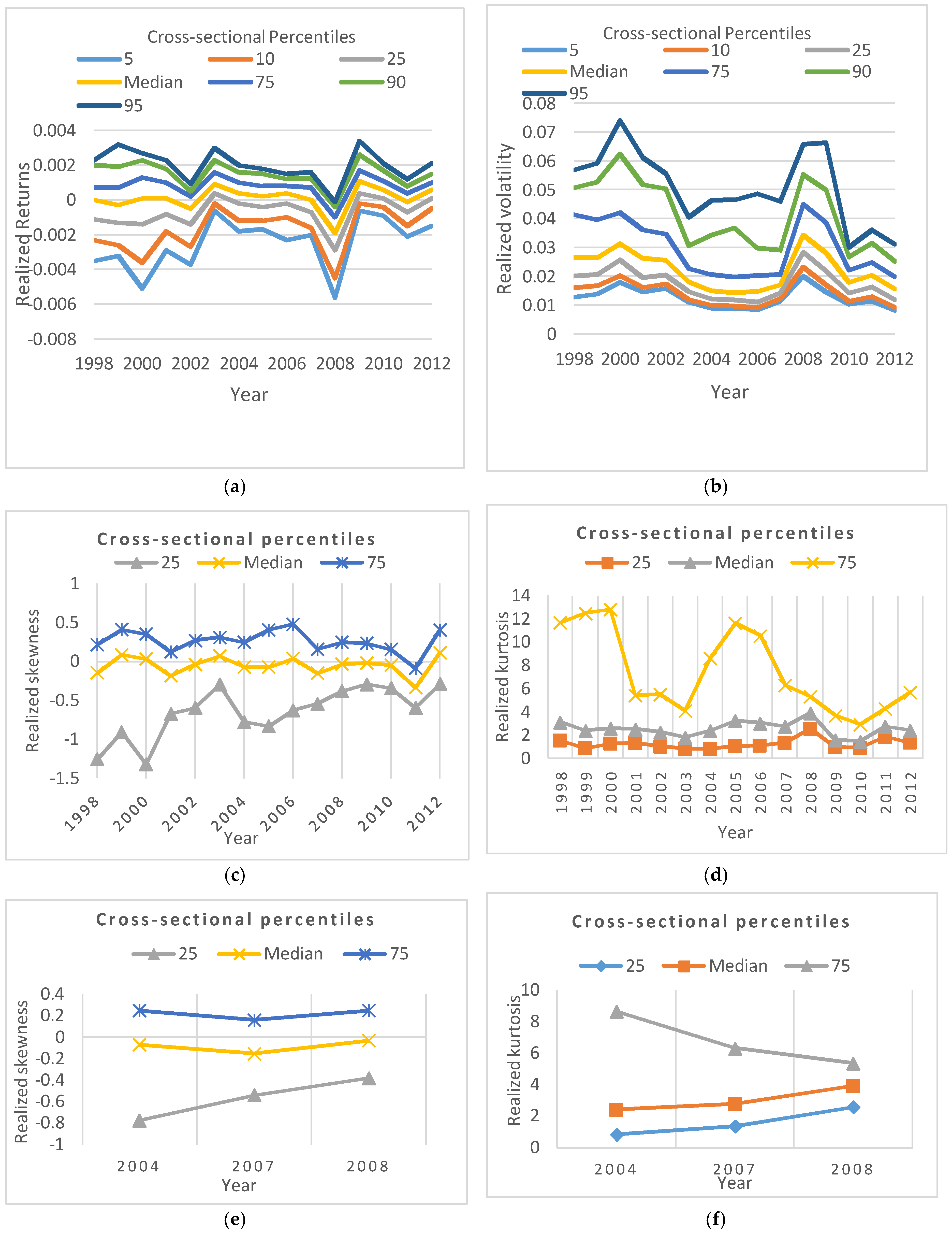
Furthermore, we investigated the cross-sectional percentiles in 250-day time windows for the frequency distribution of four moments i.e., (logarithmic returns, volatility, skewness, and kurtosis) and the graphs are shown in Figure 5.
From Figure 5a,c we can see some positive relations of realized stock returns with realized skewness. During the crisis the skewness becomes negative with stock returns; it does not happen in all cases, but most of the cases and the median shows the same result for the two graphs. However, another study found a negative relationship between realized skewness and stock returns (Amaya et al. 2015). In addition, in Figure 5b,d we can observe a positive relationship of volatility with realized kurtosis i.e., the kurtosis and volatility increase during the crisis periods and the median also shows the same result, but if we follow the 75th percentile of Figure 5d it is completely opposite to our decisions. Furthermore, we also made the percentiles of distribution of skewness and kurtosis in Figure 5e,f specifically for the years 2004, 2007, and 2008. In addition, in case of skewness, for the year 2008 if we follow Figure 5a,c the relationship was not affected in year 2008 and that finding supports the same statement in another study (Omed and Song 2014). In addition, another significant finding from Table 1 is the shape statistics features i.e., skewness for the moments (realized returns and realized skewness) is negatively increasing or more negatively skewed from the years 2004 to 2007 and kurtosis increases positively for the same years. All these findings could be a good indicator of an upcoming crisis. In addition, these characteristics reflect the features of frequency and normal distributions of stock returns.
So finally, our discussion concludes that the negative skewness and kurtosis increment of daily stock price returns can be a good indicator of future risk or crisis period for both researchers and investors.
3. Conclusions
In this paper, we tried to show the correlation among the stocks prices and beta-coefficients between the market index and the stock prices in both real and absolute volatility and also made a good comparison between stock return and volatility distribution to show the frequency behavior of stock returns from non-crisis to crisis period. We drew both frequency and bell curves for real stock returns and real volatility, and tested the skewness and kurtosis for all the stocks. Finally, we concluded that the frequency or normal distribution of daily stock return methods are good indicators of market risk because they clearly show the fat-tail and kurtosis behavior of market price fluctuations. The correlation and beta-coefficients of daily stock prices returns are also clearly explained during crisis and non-crisis periods. Our analytic comparison of this paper will provide researchers and investors with a more complete understanding of their choices when using stock returns as a risk indicator.
Author Contributions
Conceptualization, A.N. and N.A.; Methodology, A.N. and N.A.; Software, N.A.; Formal Analysis, N.A.; Resources, A.N.; Data Curation, A.N., N.A.; Writing-Original Draft Preparation, N.A.; Writing-Review & Editing, A.N. and N.A.; Supervision, A.N.; Project Administration, A.N.; Funding Acquisition, A.N.
Funding
This research was partially funded by Research Cell, Noakhali Science and Technology University, Noakhali-3814, Bangladesh.
Acknowledgments
We would like to thank Research Cell, Noakhali Science and Technology University, Noakhali-3814, Bangladesh for their partial grant in the support of Master Degree Thesis of Nahida Akter.
Conflicts of Interest
The authors declare no conflicts of interest.
References
- Amaya, Diego, Peter Christoffersen, Kris Jacobs, and Aurelio Vasquez. 2015. Does realized skewness predict the cross-section of equity returns? Journal of Financial Economics 118: 135–67. [Google Scholar] [CrossRef]
- Anderson, Spencer. 2000. A History of the Past 40 Years in Financial Crises. IFR International Financing Review IFR 2000 Issue Supplement. Available online: http://www.ifre.com/a-history-of-the-past-40-years-in-financial-crises/21102949.fullarticle (accessed on 5 March 2018).
- Ang, Andrew, and Geert Bekaert. 2007. Return predictability: Is it there? The Review of Financial Studies 20: 651–707. [Google Scholar] [CrossRef]
- Ang, Andrew, and Jun Liu. 2007. Risk, return and dividends. Journal of Financial Economics 85: 1–38. [Google Scholar]
- Azizian, Abassi. 2006. Investigating the factors determining price coefficient to the profit of listed companies on Tehran Stock Exchange. Master’s thesis, Shahid Beheshti University, Tehran, Iran. [Google Scholar]
- Batten, Jonathan A., Harald Kinateder, Peter G. Szilagyi, and Niklas Wagner. 2018. Addressing COP21 using a Stock and Oil Market Integration Index. Energy Policy 116: 127–36. [Google Scholar] [CrossRef]
- Campbell, John Y., and Samuel B. Thompson. 2008. Predicting the equity premium out of sample: Can anything beat the historical average? The Review of Financial Studies 21: 1509–31. [Google Scholar] [CrossRef]
- Cochrane, John H. 2008. The dog that did not bark: A defense of return predictability. The Review of Financial Studies 21: 1533–75. [Google Scholar] [CrossRef]
- Constantinou, Eleni, Robert Georgiades, Avo Kazandjian, and Georgios P. Kouretas. 2006. Regime switching and artificial neural network for ecasting of the Cyprus Stock Exchange daily returns. International Journal of Finance & Economics 11: 371–83. [Google Scholar]
- Drakos, Anastassios A., Georgios P. Kouretas, and Leonidas P. Zarangas. 2010. Forecasting financial volatility of the Athens stock exchange daily returns: An application of the asymmetric normal mixture GARCH model. International Journal of Finance & Economics 15: 331–50. [Google Scholar]
- Glosten, Lawrence R., Ravi Jagannathan, and David E. Runkle. 1993. On the Relation between the Expected Value and the Volatility of the Nominal Excess Return on Stocks. The Journal of Finance 48: 1779–801. [Google Scholar] [CrossRef]
- Green, T. Clifton, and Stephen Figlewski. 1999. Market Risk and Model Risk for a Financial Institution Writing Options. The Journal of Finance 54: 1465. Available online: http://www.investopedia.com/terms/v/volatility.asp (accessed on 5 March 2018).
- Huang, Jui-Chung. 2009. A fuzzy GARCH model applied to stock market scenario using a genetic algorithm. Expert Systems with Applications 36: 11710–17. [Google Scholar] [CrossRef]
- Matías, Jose M., and Juan C. Reboredo. 2012. Forecasting performance of nonlinear models for intraday stock returns. Journal of Forecasting 31: 172–88. [Google Scholar] [CrossRef]
- Nasrollahi, Zahra. 1992. The analysis of Iran stock exchange performance. Master’s thesis, Tarbiat Modares University, Tehran, Iran. [Google Scholar]
- Nobi, Ashadun, and Jae Woo Lee. 2017. Systemic risk and hierarchical transitions of financial networks. Chaos 27: 063107. [Google Scholar] [CrossRef] [PubMed]
- Omed, Amir, and Jiayin Song. 2014. Investors’ pursuit of positive Skewness in Stock Returns-An Empirical Study of the Skewness Effect on Market-to-Boo Ratio. Master’s thesis, University of Gothenburg, Gothenburg, Sweden. Master Degree Project in Finance. [Google Scholar]
- Pástor, Lubos, and Robert F. Stambaugh. 2009. Predictive systems: Living with imperfect predictors. Journal of Finance 64: 1583–628. [Google Scholar] [CrossRef]
- Roll, Richard. 1988. R2. The Journal of Finance 43: 541–66. [Google Scholar] [CrossRef]
- Sonney, Frédéric. 2009. Financial analysts’ performance: Sector versus country specialization. The Review of Financial Studies 22: 2087–131. [Google Scholar] [CrossRef]
- Summers, Lawrence H. 1996. Does the stock market rationally reflect fundamental values? Journal of Finance 41: 591–601. [Google Scholar] [CrossRef]
- Van Binsbergen, Jules H., and Ralph S. J. Koijen. 2010. Predictive regressions: Apresent value approach. Journal of Finance 65: 1439–71. [Google Scholar] [CrossRef]
- Zahedi, Javad, and Mohammad Mahdi Rounaghi. 2015. Application of artificial neural network models and principal component analysis method in predicting stock prices on Tehran Stock Exchange. Physica A: Statistical Mechanics and its Applications 438: 178–87. [Google Scholar] [CrossRef]
Figure 1.
Average beta-coefficient of S&P 500 377 stocks with market index over year 1998 to 2012.

Figure 2.
Stock behavior with market index returns over non-crisis, before-crisis, and crisis years.
Figure 2.
Stock behavior with market index returns over non-crisis, before-crisis, and crisis years.

Figure 3.
Average correlation of S&P 500, 377 stocks over year 1998 to 2012.

Figure 4.
(a) Frequency and normal distribution of stock returns during non-crisis year 2004; (b) Frequency and normal distribution of stock returns volatility non-crisis year 2004; (c) Frequency and normal distribution of stock returns before crisis year 2007; (d) Frequency and normal distribution of stock returns volatility before crisis year 2007; (e) Frequency and normal distribution of stock returns during crisis year 2008; (f) Frequency and normal distribution of stock returns volatility during crisis year 2008.


Figure 5.
250-day cross-sectional percentiles of frequency distribution. (a) Realized stock returns; (b) Realized volatility; (c) Realized skewness; (d) Realized kurtosis; (e) Realized skewness for the year 2004, 2007 and 2008; (f) Realized kurtosis for the year 2004, 2007 and 2008.
Figure 5.
250-day cross-sectional percentiles of frequency distribution. (a) Realized stock returns; (b) Realized volatility; (c) Realized skewness; (d) Realized kurtosis; (e) Realized skewness for the year 2004, 2007 and 2008; (f) Realized kurtosis for the year 2004, 2007 and 2008.


Table 1.
Descriptive statistics analysis: Non-crisis year (2004), before crisis (2007) and crisis year (2008).
Table 1.
Descriptive statistics analysis: Non-crisis year (2004), before crisis (2007) and crisis year (2008).
| Year | Features | Realized Returns | Realized Volatility | Realized Skewness | Realized Kurtosis |
|---|---|---|---|---|---|
| 2004 | Mean | 0.0004 | 0.0188 | −1.4819 | 23.9337 |
| Median | 0.0004 | 0.0149 | −0.0721 | 2.3868 | |
| Std. Deviation | 0.00115 | 0.01067 | 3.94839 | 56.12373 | |
| Skewness | 0.004 | 1.760 | −2.366 | 2.643 | |
| Kurtosis | 2.052 | 2.324 | 4.315 | 5.545 | |
| 2007 | Mean | −0.0001 | 0.0195 | −1.1261 | 19.3739 |
| Median | 0 | 0.017 | −0.1546 | 2.7714 | |
| Std. Deviation | 0.00124 | 0.00966 | 3.49547 | 48.95879 | |
| Skewness | −0.766 | 2.518 | −2.568 | 3.039 | |
| Kurtosis | 3.258 | 7.103 | 6.606 | 7.879 | |
| 2008 | Mean | −0.0022 | 0.0380 | −0.1428 | 5.5175 |
| Median | −0.0019 | 0.0344 | −0.0350 | 3.9136 | |
| Std. Deviation | 0.00175 | 0.01437 | 0.93757 | 9.07936 | |
| Skewness | −1.618 | 1.499 | −4.824 | 8.682 | |
| Kurtosis | 5.554 | 3.336 | 36.907 | 91.016 |
© 2018 by the authors. Licensee MDPI, Basel, Switzerland. This article is an open access article distributed under the terms and conditions of the Creative Commons Attribution (CC BY) license (http://creativecommons.org/licenses/by/4.0/).
Share and Cite
MDPI and ACS Style
Akter, N.; Nobi, A. Investigation of the Financial Stability of S&P 500 Using Realized Volatility and Stock Returns Distribution. J. Risk Financial Manag. 2018, 11, 22. https://doi.org/10.3390/jrfm11020022
AMA Style
Akter N, Nobi A. Investigation of the Financial Stability of S&P 500 Using Realized Volatility and Stock Returns Distribution. Journal of Risk and Financial Management. 2018; 11(2):22. https://doi.org/10.3390/jrfm11020022
Chicago/Turabian StyleAkter, Nahida, and Ashadun Nobi. 2018. "Investigation of the Financial Stability of S&P 500 Using Realized Volatility and Stock Returns Distribution" Journal of Risk and Financial Management 11, no. 2: 22. https://doi.org/10.3390/jrfm11020022