
Volatility Forecast in Crises and Expansions

Department of Economics, University of Western Ontario, Social Science Centre Rm 4064, London, N6A5C2, Canada
J. Risk Financial Manag. 2015, 8(3), 311-336; https://doi.org/10.3390/jrfm8030311
Submission received: 26 February 2015
/
Revised: 30 May 2015
/
Accepted: 6 July 2015
/
Published: 5 August 2015
(This article belongs to the Special Issue Financial Risk Modeling and Forecasting)
Abstract
:We build a discrete-time non-linear model for volatility forecasting purposes. This model belongs to the class of threshold-autoregressive models, where changes in regimes are governed by past returns. The ability to capture changes in volatility regimes and using more accurate volatility measures allow outperforming other benchmark models, such as linear heterogeneous autoregressive model and GARCH specifications. Finally, we show how to derive closed-form expression for multiple-step-ahead forecasting by exploiting information about the conditional distribution of returns.
1. Introduction
Volatility plays an important role in financial econometrics. Measuring, modelling and forecasting financial volatility are essential for risk management purposes, portfolio allocation and option pricing. Although returns remain unpredictable, their second moment can be forecasted quite accurately, which generated a lot of research during the last thirty years motivated by Engle’s seminal paper [1]. The existing literature aiming to model and forecast financial volatility can be divided into two distinct groups: parametric and non-parametric models. The former assumes a specific functional form for volatility and models it as a function of observable variables, such as ARCH or GARCH models [1,2,3], or as a known function of latent variables resulting in stochastic volatility models [4,5].
The second class defines financial volatility without imposing any parametric assumptions hence called realized volatility models [6]. The main idea of the latter models is to construct consistent estimators for the unobserved integrated volatility by summing the squared returns over a very short period within a fixed time span, typically one day. The availability of high-frequency data allows high precision estimation of the continuous time pure diffusion processes given the large datasets of discrete observations. As a result, volatility essentially becomes observable and, in the absence of microstructure noise, can be consistently estimated by a realized volatility measure. This approach has two main benefits compared with GARCH and stochastic volatility models. First, researchers can treat volatility as observable and model it by applying a time series technique, for example ARFIMA or autoregressive fractionally integrated moving average models [6]. Second, realized volatility models significantly outperform models based on lower frequency (daily data) in terms of forecasting power; see, e.g., [7,8,9]. Indeed, the latter models adapt new information and update the volatility forecast at a slower daily frequency, while the former models can incorporate changes in volatility faster due to the more frequent arrival of intraday information.
Although the literature proposes many different approaches for modelling volatility, there is still no unique model that explains all of the stylized facts simultaneously. In particular, there is no consensus on how to model long memory, since there are at least four approaches: the non-linear model with regime switching [9]; the linear fractionally-integrated process [10]; the mixture of heterogeneous run information arrivals [11]; and the aggregation of short memory stationary series [12]. Numerous methods have been developed, since it is hard to distinguish between unit root and structural break data generating processes [13,14]. [15] show that structural break models can outperform the long memory model if the timing and sizes of future breaks are known. Although few academics and practitioners accurately predicted the timing of the recent financial crises and European sovereign debt turmoil, a model with structural breaks seems to be more economically plausible than a fractionally-integrated long memory model. In addition, [15] recommend relying on economic intuition to choose between smooth transition auto regressive models (STAR) and abrupt structural break models.
In this paper, we extend the heterogeneous autoregressive model proposed by [16] to take into account different regimes of volatility. The resulting model is called a non-linear threshold autoregression model, where regimes are governed by an exogenous trigger variable. This model provides a better fit of the robust measure of realized volatility for both in-sample data and out-of-sample forecasting. In addition to an improved performance in particular samples, a non-linear model also produces superior multiple-step-ahead forecasts in population according to the Giacomini and White test [17]. We also show that the superior performance of a non-linear model is achieved during periods of high volatility. This is especially important during times of financial crises, when investors are in particular need of more accurate forecasts. Finally, we derive a closed form expression for multiple-step-ahead forecast, where the past returns govern changes in volatility regimes.
Our paper finds that changes in the volatility regimes occur when return exceeds a −1% threshold, which is in line with previous findings [9,18]. However, our model differs in terms of the estimation procedure and the most recent dataset that includes financial crises. In fact, the superior performance of a non-linear model becomes particularly significant during periods of elevated volatility, such as recent financial crises. More importantly, we a derive a closed-form expression of multiple-step-ahead forecasts, whereas other authors either focus on one-step ahead forecasts [9] or using conditional simulations [18].
The remainder of this paper is organized as follows. The non-linear threshold model for realized volatility is defined in Section 2. Section 3 describes preliminary data analysis and estimation results for the S&P 500 index. Section 4 describes one and multiple-step-ahead forecasts. Finally, Section 5 concludes and provides directions for future work.
2. Model
In this section, we introduce two building blocks: the heterogeneous autoregressive model and the regime switching model. Then, we describe the econometric framework designed for the estimation and inference of our threshold autoregressive model. Finally, we discuss the forecasting of our model and how to derive a closed form expression for its multiple-days-ahead forecasts.
2.1. HAR-RV Model with Regime Switching
In this section, we discuss extensions of the heterogeneous autoregressive model (HAR) of realized volatility proposed in [16]. First, let us assume that returns follow a continuous diffusion process:
where is the logarithm of instantaneous price, is continuous with a finite variation mean process, is instantaneous volatility and is standard Brownian motion. Given the process in (1), the integrated variance corresponding to day t is defined as:
Several authors show that as sampling frequency increases, integrated volatility can be approximated by realized variance defined as a sum of the intraday squared returns [6,19,20]. In essence, volatility becomes observable and can be forecasted using time series techniques.
The presence of market microstructure noise makes realized variance inconsistent and is a biased estimator of true volatility. Therefore, we use the realized kernel estimator developed in [21], which remains consistent under the presence of market microstructure noise. The realized kernel is an estimator of latent realized variance and is defined as follows:
where , is a weight function and is i-th intra-daily log price sampled at frequency δ and recorded at day t. In other words, and , where is the number of seconds during the trading day. Thus, the realized kernel is similar to the HAC (heteroskedasticity and autocorrelation consistent covariance matrix) estimator of the variance-covariance matrix for some stationary time series. Throughout this paper, realized variance will equal the realized kernel measure defined in Equation (3).
The realized kernel has several advantages over other high-frequency proxies of latent volatility. First, [22] show that the realized kernel performs better (in terms of forecasting value-at-risk) than other high-frequency measures, including realized volatility, bi-power realized volatility, two-scales realized volatility and daily range. Second, the realized kernel is a consistent estimator of latent variance, which is robust to the market microstructure noise.
The heterogeneous autoregressive model is able to replicate the majority of stylized facts observed in data: fat tails, volatility clustering and long memory. In particular, HAR is able to generate hyperbolic decays in the autocorrelation function in a parsimonious way due to the volatility cascade property, despite the fact that this model does not belong to the class of long memory models. This model is based on the heterogeneous market hypothesis [23] , which implies that lower frequency volatility (weekly) affects higher frequency volatility (daily), but not vice versa:
where , and are daily, weekly and monthly realized variance, respectively, at period t. The lower frequency, for example weekly, realized variance is computed as:
Similarly, the monthly realized variance is computed as the average of daily variances over 22 days. Although the HAR model is able to capture long memory and volatility clustering, it cannot explain abrupt changes in regimes. Indeed, recent subprime mortgage crises, European debt turmoil and a number of other financial calamities led to significantly different behaviour in the dynamics of the realized volatility during “good” and “bad” times, as we will discuss in Section 3. Therefore, we propose to extend the benchmark HAR model and allow the possibility of multiple regimes, governed by either endogenous or exogenous variables. We define the threshold HAR model with two regimes as follows:
where is a trigger variable with some lag l and τ is the value of a threshold. In this paper, we consider only observable triggers, including returns and the realized kernel.
2.2. Econometric Framework for the Non-Linear Model
2.2.1. Estimation
Next, we present the econometric techniques designed to model non-linear dynamics of time series: the self-exciting threshold autoregressive (SETAR) model and the threshold autoregressive (TAR) model introduced by [24] and [25]. The main difference between these models is that the trigger variable can be either exogenous (TAR model) or endogenous (SETAR model). The TAR(m) model, where m denotes the number of regimes, is defined as follows:
where is a univariate time series, vector, and , , is an indicator function and is a threshold variable. Let us assume that and , while the error term is conditionally independent on information set and has a finite second moment:
In particular, if variable follows the TAR(2) process, then the model (7) becomes:
Recall that Model (9) nests a non-linear HAR specification (6) if we put constraints on the corresponding AR(22) model in each regime. Now, define the vector of all parameters of Model (9) as . Under Assumption (8), the estimation of the TAR(m) model is performed using a non-linear least squares approach:
Here, the minimization can be done sequentially. In particular, can be computed through OLS regression of Y on for fixed parameters d and τ:
where Y is the Tx1 vector consisting of observations of , while is the Tx matrix with t-th row :
Now, let us assume for simplicity that the non-linear model has only two regimes or . Thus, two parameters τ and l can be estimated through minimization of the residual sum of squared errors :
where .
The minimization can be performed through a grid search, while noting that l is discrete. We follow [26] approach, which allows speeding up the minimization algorithm. In particular, he recommends eliminating the smallest and largest quantiles for the threshold variable in the grid search. This elimination does not only reduce the computational time, but also serves as a necessary condition for having enough observation in each regime. Indeed, asymptotic theory places additional constraints on the optimal threshold level, such that as . Although, there is no clear procedure for how to optimally choose τ, [26] recommends to use a 10% quantile for the cut-off procedure.
2.2.2. Testing for Non-Linearity
We start by discussing the testing of the linear model or TAR(1) against the non-linear model or TAR(m), where . Under the null hypothesis, all parameters , ..., should be the same:
Since the threshold parameter is not identified under the null hypothesis, the classical tests have a non-standard distribution. This problem is called “Davies’ problem” due to [27,28]. [26,29] overcomes this problem by using empirical process theory and derived the limiting distribution of the main statistics of interest :
where and are the sum of squared residuals and . Computation of the asymptotic distribution is not straightforward, but might be faster than a bootstrap calculation. Although the literature does not assess the performance of the asymptotic against the bootstrap distribution in the context of SETAR models, [30] show that the bootstrap technique performs better in the AR(1) context with Andrews structural change test [31]. Thus, we use the following bootstrap algorithm for testing the linear model against the non-linear TAR(2) model:
- Draw residuals with replacement from the linear TAR(1) model.
- Generate a recursively “fake” dataset using initial conditions and estimates of the TAR(1) model, where p equals 22.
- Estimate the TAR(1) and TAR(2) models on the “fake” dataset.
- Compute and on the fake dataset, where b refers to specific bootstrap replication.
- Compute statistics from (15).
- Repeat Steps (1)–(5) a large number of times.
- The bootstrap p-value () equals the percentage of times that exceeds the actual statistic .
The algorithm in (1)–(7) can be used to evaluate the distribution of under the assumption of either homoscedastic or heteroscedastic errors. We compute the bootstrap p-value under the latter assumption, since the residuals of Model (4) are heteroscedastic. This is in line with the literature [32]. These diagnostic tests are available upon request.
2.2.3. Testing for Remaining Non-Linearity
The testing for remaining non-linearity is an important diagnostic check for the TAR (m) model. One way to address this question is to test whether the presence of the additional regime is statistically significant or not. This test relies on the aforementioned algorithm, while the bootstrap p-value is computed for statistics , where .
2.2.4. Asymptotic Distribution of the Threshold Parameter
The existing literature documents that the distribution of the parameter τ is non-standard if the threshold effect is significant [26,33]. [29,34] derives an asymptotic distribution of likelihood ratio statistics:
where is the residual sum of squares given parameter τ and is the variance of residuals of the TAR(2) model and equals . Moreover, [29,34] shows that the confidence interval for the threshold parameter is obtained by inverting the distribution function of a limiting random variable. In other words, the null hypothesis is rejected if the likelihood ratio exceeds the function of confidence level α:
Alternatively, the confidence interval for the threshold parameter is formed as an area where and is called the “no-rejection region”. We have to interpret the confidence interval for threshold parameter τ with caution, since it is typically conservative [26,29]. However, the ultimate test of our non-linear model is the ability to produce superior out-of-sample forecasts, which requires a tight confidence interval for the threshold parameter. We provide more discussion on page 15.
Although estimates depend on the threshold parameter τ, the asymptotic distribution remains the same as in the linear model case, since estimate is super-consistent [35]. [33] and [26] prove that dependency on the threshold parameter is not of first order asymptotic importance, thus the confidence interval for can be constructed as if is a known parameter.
2.2.5. Stationarity
The stationarity conditions for our TAR(2) model are not easily derived, and in general, not much is known about this property for non-linear models with heteroskedastic errors—see the discussion in [35] (pp. 79–80). The literature does propose sufficient conditions for a restricted class of non-linear models and typically for models with homoscedastic errors. In particular, [36] consider SETAR(2) specification with the AR(1) model in both regimes, while [37] establish necessary and sufficient conditions for the existence of a stationary distribution for TAR(2) and SETAR(2) models with the AR(1) process.
In contrast, our model has a richer structure within each regime, since the HAR model is a restricted version of the AR(22) process. Because of this richer structure within each regime and because neither self-exciting nor exogenous thresholds are used, it is not possible to use the results from [36] and [37] to prove stationarity. In addition, our residuals exhibit volatility clustering, and because of the heteroscedastic errors, it is not possible to exploit the necessary and sufficient conditions for strict stationarity, even for the simple HAR model derived by [9]. The diagnostic checks show that this assumption does not hold.
In conclusion, as is the case in much empirical work, we have to make a trade-off between the flexibility of the model and the analytical tractability of stationarity conditions. In this paper, we choose to design a model aiming at providing more accurate volatility forecasts, and we leave the question of stationarity for future work.
2.3. Forecasting
2.3.1. One-Step-Ahead Forecast
We assess the forecasting performance of various models by computing the one-step-ahead forecast of the realized volatility measured by the square root of the realized kernel. These forecasts are computed through rolling window estimation. First, the parameters of the model are estimated using an in-sample set, and then the one-step-ahead forecast is computed. Second, the rolling window is moved by one period ahead; the most distant observation is dropped, and the parameters of the model are re-estimated, while the threshold parameter τ and optimal lag l are kept time invariant. Finally, the one-step-ahead forecast is computed again.
We use the root mean square error (RMSE) and the mean absolute error (MAE) to compare the forecast performance of four models:
where is the one-step-ahead conditional forecast of the daily realized volatility computed based on the rolling window for one of the four models and is the daily realized volatility at period . In addition, we compute of the following Mincer–Zarnowitz regression:
Finally, we investigate the forecasting performance of different models in population using the Giacomini and White (GW) test [17]. The GW test fits nicely in our framework due to the following reasons. First, it does not favour models that overfit in-sample, but have high estimation errors. Second, this test is designed to compare not only unconditional, but conditional forecasts, as well. Finally, the GW test works with rolling window forecasts, where in-sample size is fixed, while out-of-sample size is growing.
2.3.2. Conditional Distribution of Returns
In this section, we discuss multiple-step-ahead forecasts for aggregate volatility over periods of five and 10 days. The extension of the multiple-step-ahead forecast to the linear model is straightforward, while the non-linear model has one important problem. We describe formulas used to compute the multiple-step-ahead forecast for the HAR, GARCH(1,1) and GJR-GARCH(1,1) (proposed by [38]) models in Appendix A. In particular, the one-step-ahead forecast remains the same for both non-linear and linear cases, while the two-step-ahead one is different:
where is the information set available at period t, F is a non-linear function, θ is a vector of estimates and is the realized volatility at period t. Equation (19) illustrates the main problem related to non-linear model: the expected value of a non-linear function differs from the value of a non-linear function evaluated at the expected value. In the literature, several methods have been proposed for the computation of the multiple-step-ahead forecast, including conditional simulations in [18]. However, we choose a different strategy and derive a closed form solution for the multiple-step forecast. Specifically, we follow an approach similar to [39] and [40] to derive the conditional distribution of returns. Given the diffusion process (1), the standardized returns should follow a normal distribution:
where is information at the period t set generated by the history of returns and is the mean of standardized returns, and and should be close to zero and one, correspondingly. See Table B1 in Appendix B for details. Meanwhile, the conditional distribution of realized volatility is closely approximated by the inverse Gaussian distribution with the following density function:
where is a conditional mean and is a shape parameter of the inverse Gaussian distribution. The conditional mean is assumed to be filtered from the non-linear TAR(2) model as follows:
Combining Equations (20) and (21), the conditional distribution of returns becomes a normal-inverse Gaussian distribution (NIG) with the probability density function computed as:
The NIG distribution provides a relatively accurate fit of the unconditional distribution of returns (see Appendix B for details). Having the distributional assumption for returns, Theorem 1 demonstrates how to obtain the closed form expression for the multiple-step ahead forecast of the realized volatility.
Theorem 1. Let follow the TAR(2) process defined in (6), while returns follow the NIG distribution with the conditional probability density function defined in (23), and () are independent of ,...,. Then, the h-step-ahead forecast () is obtained as follows:
where:
Proof. See Appendix C. ☐
In essence, Formula (24) is similar to the multiple-step-ahead forecast of the GJR-GARCH(1,1) model — see Appendix A for details. However, the TAR model has an additional flexibility, since probability is time varying, while GJR-GARCH assumes that the corresponding probability equals to 0.5. To facilitate comparison between these two models, we compute the unconditional probability of a high volatility regime occurring based on the NIG distribution (23) and from returns data. Here, the probability equals the frequency of returns occurring, which is lower than the threshold value. The results show a close match between these two methods: 11.3% (NIG) vs. 13.2% (historical returns) for in-sample data.
Finally, we describe the multiple-step-ahead forecast using the rolling window approach. First, the parameters of the model are estimated using in-sample data, and probability is computed. Second, multiple-step-ahead forecasts for the TAR model are calculated based on Expression (24), while remains constant. Probability can be computed for each step of forecast, as well, but this will add additional computational burden, while the results should change only marginally. In other words, we assume that , where . We compute h-step-ahead forecasts for the HAR, GARCH(1,1) and GJR-GARCH(1,1) models based on the formulas presented in Appendix A. Finally, the rolling window is moved by one period ahead; the first observation is dropped, and the parameters of the model, including , are re-estimated.
3. Empirical Analysis
3.1. Data
The empirical analysis is based on high-frequency data for the S&P 500 index obtained through the Realized Library of Oxford-Man Institute of Quantitative Finance (Library Version 0.2), which is freely available:
“Researchers may use this library freely without restrictions so long as they quote in any work which uses it: Heber, Gerd, Asger Lunde, Neil Shephard and Kevin Sheppard (2009) “Oxford-Man Institute’s realized library”, Oxford-Man Institute, University of Oxford.”
The sample covers the period from 3 January of 2000 to 12 June of 2014, overall 3603 trading days. We exclude all days from the sample when the market was closed. [41] have created the Realized Library database, which provides daily data for about 11 realized measures for 21 assets. The authors clean the raw data obtained through Reuters Data Scope Tick History and compute high-frequency estimators from cleaned data. We use a realized kernel [21] as a proxy for integrated variance.
3.2. Preliminary Data Analysis
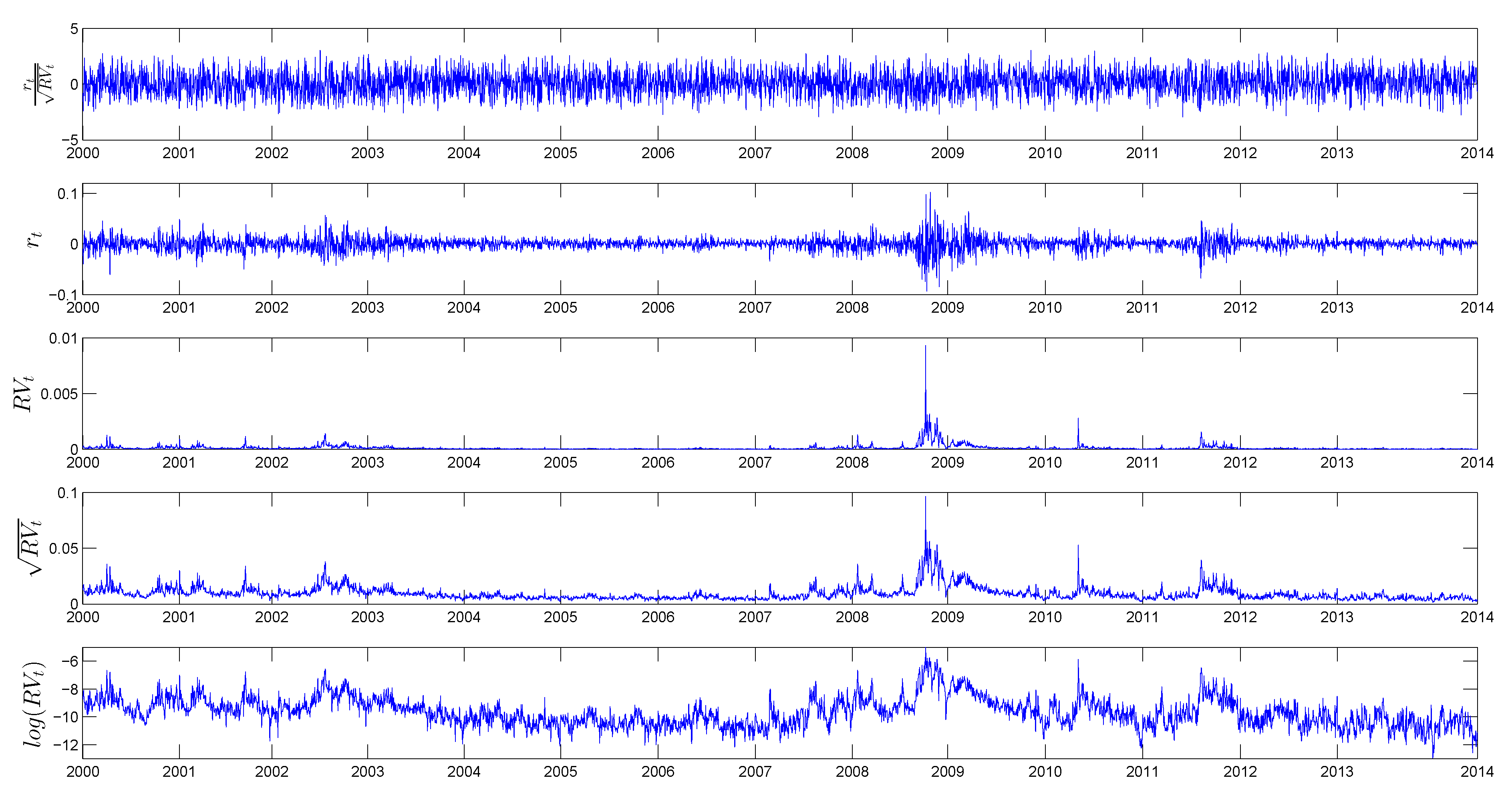
We start with data analysis of five main time series of interest: standardized returns, returns, realized variance, realized volatility and the logarithm of realized variance. Table 1 presents the descriptive statistics, while Figure 1 illustrates the time series dynamics of these variables.

| Mean | 0.08 | 8.0E-05 | 1.2E-04 | 9.3E-03 | −9.65 |
| Variance | 1.19 | 1.5E-04 | 7.5E-08 | 3.8E-05 | 1.08 |
| Skewness | −3.3E-03 | −0.15 | 14.26 | 3.32 | 0.50 |
| Kurtosis | 2.57 | 10.24 | 381.25 | 24.58 | 3.47 |
| D-F test | p = 0.00 | p = 0.00 | p = 0.00 | p = 0.00 | p = 0.06 |
| Normality test (J-Btest) | p = 0.00 | p = 0.00 | p = 0.00 | p = 0.00 | p = 0.00 |
| L-Btest 5 lags | p = 0.01 | p = 0.00 | p = 0.00 | p = 0.00 | p = 0.00 |
| L-B test 10 lags | p = 0.08 | p = 0.00 | p = 0.00 | p = 0.00 | p = 0.00 |
| L-B test 15 lags | p = 0.07 | p = 0.00 | p = 0.00 | p = 0.00 | p = 0.00 |
| ARCH effect | p = 0.00 | p = 0.00 | p = 0.00 | p = 0.00 | p = 0.00 |
Four of the variables are stationary at 5% according to the augmented Dickey–Fuller test, while is stationary at 6%. The recent financial crises and European sovereign debt turmoil affected the volatility pattern and led to several spikes in the realized variance series. Although these spikes look less pronounced in the logarithm of realized variance, they remain very distinct from the volatility behaviour observed during calm times. This observation motivates the introduction of the regime switching model for volatility process.
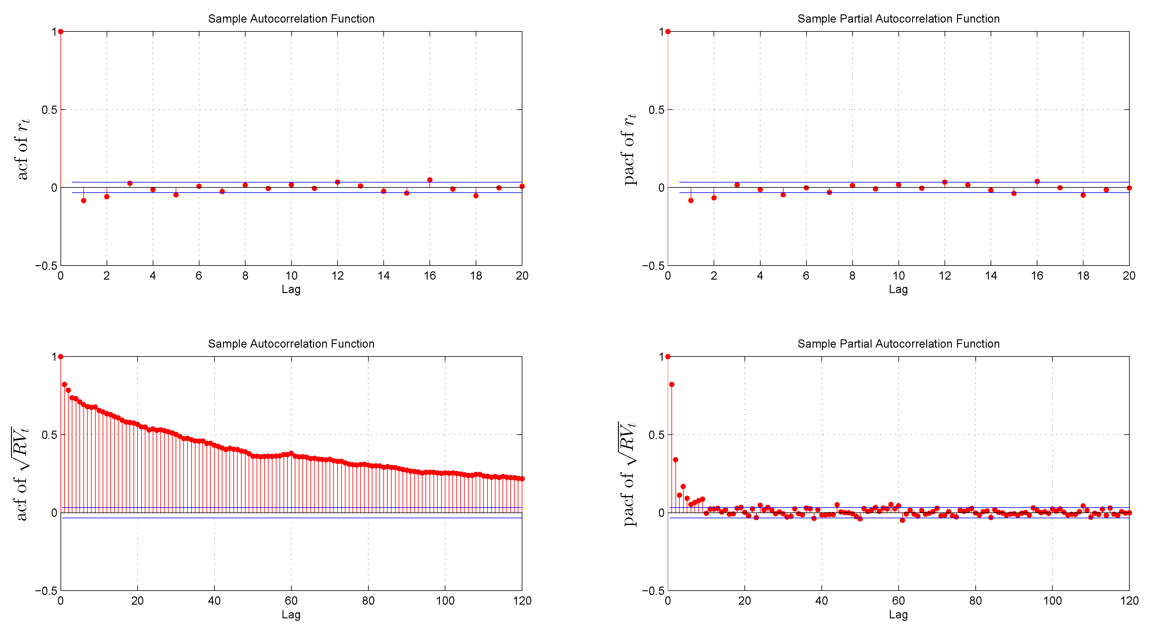
Daily returns are weakly correlated and follow a leptokurtic and negative skewed distribution. By contrast, the distribution of the standardized returns is much closer to Gaussian, which is in line with previous empirical findings: [10,42]. Figure 2 documents the long memory observed in realized volatility as the autocorrelation function decays at a hyperbolic rate. This result is also consistent with the literature: [6,15,32].
Figure 1.
Daily standardized returns, returns, realized variance, realized volatility and the logarithm of the realized variance of the S&P500 index. The sample period goes from January 2000 till June 2014 (3603 observations).
Figure 1.
Daily standardized returns, returns, realized variance, realized volatility and the logarithm of the realized variance of the S&P500 index. The sample period goes from January 2000 till June 2014 (3603 observations).

Figure 2.
Sample autocorrelations and partial autocorrelations of returns and realized volatility.

3.3. Benchmark HAR Model
We start with the estimation of the benchmark linear Model (4) for the three specifications of dependent variable , and , correspondingly. Table 2 presents the estimation results with the standard errors computed based on the HAC variance-covariance matrix.
| Estimate | SE | Estimate | SE | Estimate | SE | |
| c | 1.3E-05 | 4.5E-06 | 4.6E-04 | 2.0E-04 | −0.44 | 0.108 |
| 0.223 | 0.146 | 0.395 | 0.058 | 0.336 | 0.025 | |
| 0.461 | 0.165 | 0.384 | 0.081 | 0.440 | 0.036 | |
| 0.216 | 0.073 | 0.171 | 0.048 | 0.178 | 0.029 | |
| 50.4% | 72.6% | 73.2% | ||||
Reported are in-sample estimation results of the linear HAR model and corresponding standard errors computed based on the HAC variance-covariance matrix. The in-sample covers the period from February 2000 to June 2014 (3582 observations). Here, means that the corresponding p-value is lower than 0.01.
Despite relatively high for and , the benchmark model fails to model spikes in volatility during turbulent times on financial markets. Figure 3 illustrates this point and depicts a comparison between the in-sample forecast and the actual realized kernel.
Figure 3.
In-sample comparison of actual realized volatility (blue line) and volatility recovered from the HAR model (red line). The in-sample covers the period from February 2000 to June 2014 (3582 observations).
Figure 3.
In-sample comparison of actual realized volatility (blue line) and volatility recovered from the HAR model (red line). The in-sample covers the period from February 2000 to June 2014 (3582 observations).

In particular, benchmark Model (4) underestimates volatility by around 40% during financial crises in 2007–2009. A similar pattern is observed during spikes in volatility in 2010 and 2011. One of the explanations of the poor performance of the HAR model during turbulent volatility periods is that it fails to take into account changes in volatility regimes. Indeed, if volatility reacts to negative returns more than to positive returns, then the arrival of the consequent negative shocks and volatility persistence can substantially increase the future volatility level. On the other hand, different economic regimes might affect volatility differently. We choose the TAR over SETAR model based on the higher value of the statistics or, alternatively, the lower value of defined in Subsection 2.2.2. These results are available upon request.
3.4. The TAR(2) Model
Next, we estimate the TAR(2) model (Table 3 and Table 4), where past returns govern changes in the volatility regimes.
Table 3 shows that regression improves substantially if regimes are driven by past returns. As a result, high values of the statistics lead to the rejection of the null hypothesis (13) for all specifications at a 5% significance level. In addition, the optimal value of the threshold parameter remains the same for two specifications: and . The τ that corresponds to logarithm specification is closely related to the second threshold of the TAR(3) model. However, the confidence interval for this parameter is very wide, which leads to the imprecise estimate of the threshold parameter. Not surprisingly, this model produces a less accurate one-step forecast than TAR(2). In particular, [43] document that the imprecise estimate of the threshold parameter leads to the poor forecasting performance of the simple switching model compared to the random walk model. In both cases, changes in regimes are driven not only by negative returns (leverage effect), but by significantly negative returns: −1.3% on a daily scale. [9] also show that the transition between volatility regimes is governed not by negative past returns, but by “very bad news” or very negative past returns.
| of TAR(1) | 50.4% | 72.6% | 73.2% |
| of TAR(2) | 58.0% | 74.9% | 74.7% |
| τ | −0.013 | −0.013 | 0.001 |
| l | 0 | 0 | 0 |
| 649.6 | 318.3 | 214.0 | |
| 0.00 | 0.03 | 0.00 |
Reported are in-sample estimation results of the linear HAR model and non-linear TAR(2) model. The in-sample covers the period from February 2000 to June 2014 (3582 observations). is computed based on 500 replications using the heteroscedastic bootstrap method. We set the maximum amount of lags equal to 10 in the TAR estimation.
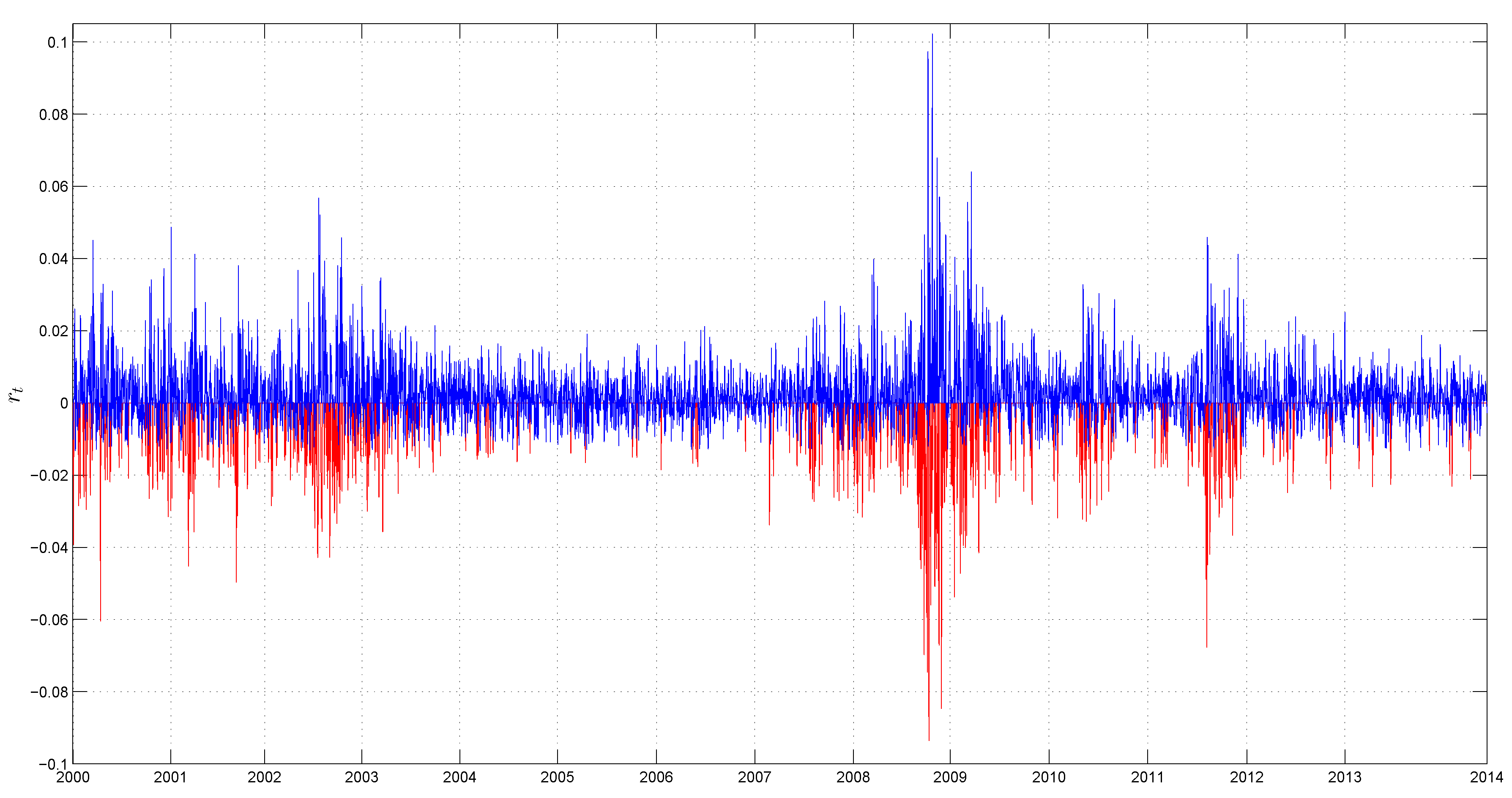
The fact that changes in regimes are triggered by “very negative returns” can be explained by the volatility persistence and higher intensity of shocks during bad times. Although the value of the threshold is not very large (it corresponds to the 11th percentile of the returns distribution), the increasing number of negative returns can generate a spike in the volatility. This explanation is similar to the option pricing literature, where researchers modelled volatility by adding infinite activity jumps to the return’s process [44]. Even though the appearance of one small or medium jump is not enough to generate a significant surge in volatility, high volatility persistence can lead to pronounced spikes in the future volatility. Indeed, Figure 4 shows that the frequency of returns that are lower than the threshold (red line) increased dramatically during recent financial crises. By contrast, returns that exceed the threshold (blue line) completely dominated “very negative returns” during the period of low volatility in 2003–2007.
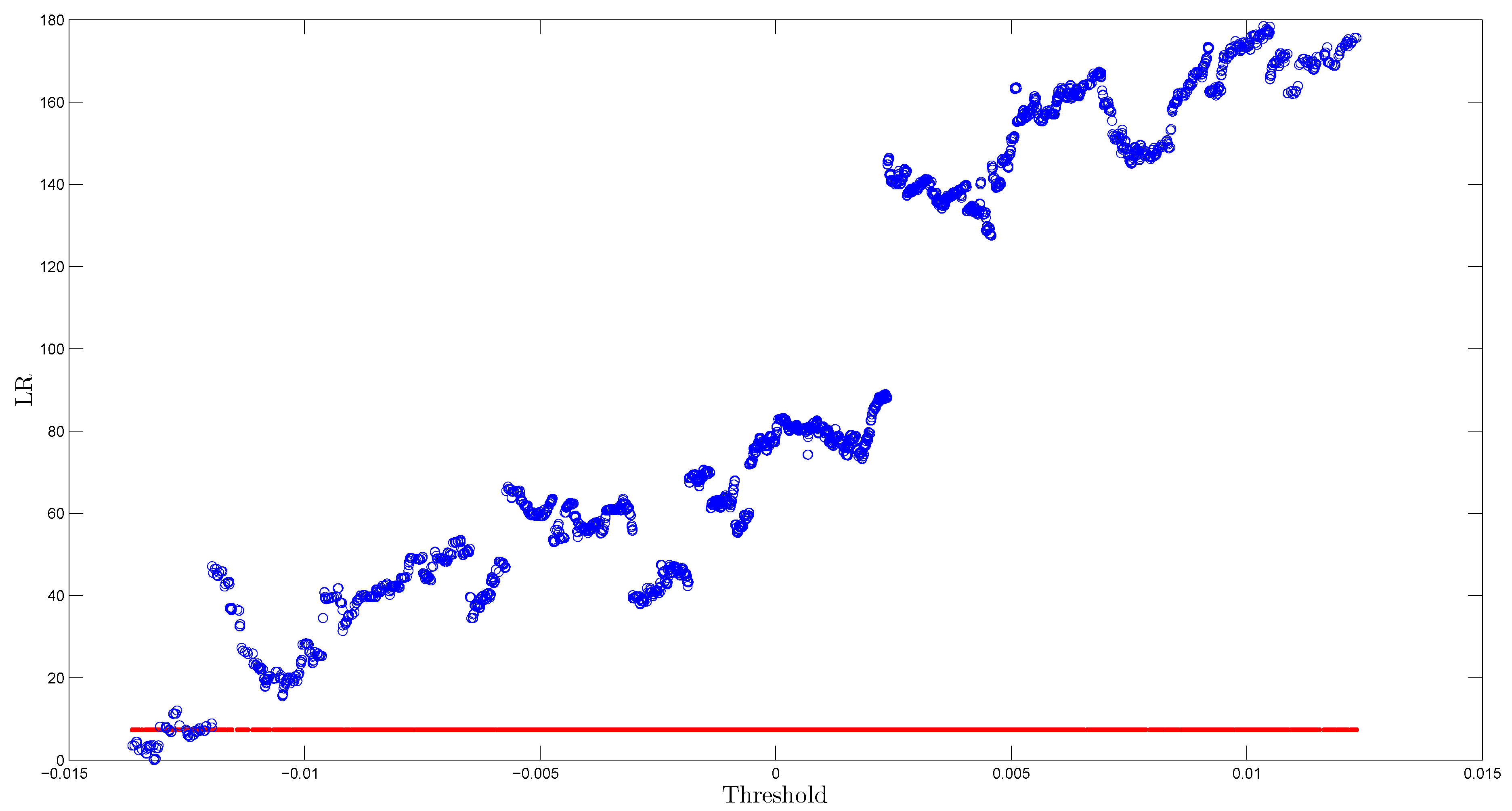
Table 4 shows that parameters , and are very different in high- and low-volatility regimes. In particular, is twice as large as the corresponding estimate in the low-volatility regime for specification. Although some estimates have negative signs, they are not statistically significant at 10% for both realized volatility and variance models. By contrast, intercepts in both regimes are statistically negative for logarithmic specifications. Overall, corresponding estimates differ substantially in different regimes, which highlights the importance of using the regime switching model. Next, Figure 5 shows that the 95% confidence interval for the threshold parameter is quite narrow (), although it includes two disjoints sets.
Figure 4.
Daily returns in high (red line) and low (blue line) volatility regimes. The high (low) volatility regime occurs when the return is lower (higher) than the threshold. The sample period goes from February 2000 till June 2014 (3603 observations).
Figure 4.
Daily returns in high (red line) and low (blue line) volatility regimes. The high (low) volatility regime occurs when the return is lower (higher) than the threshold. The sample period goes from February 2000 till June 2014 (3603 observations).

| Estimate | SE | Estimate | SE | Estimate | SE | |
| −2.6E-06 | 4.1E-05 | −9.3E-05 | 9.5E-04 | −0.321 | 0.138 | |
| 0.331 | 0.189 | 0.332 | 0.085 | 0.347 | 0.029 | |
| 1.091 | 0.372 | 0.811 | 0.191 | 0.475 | 0.045 | |
| −0.138 | 0.275 | −0.018 | 0.128 | 0.133 | 0.037 | |
| 2.1E-05 | 5.6E-06 | 0.001 | 1.8E-04 | -0.515 | 0.150 | |
| 0.182 | 0.156 | 0.340 | 0.067 | 0.220 | 0.038 | |
| 0.260 | 0.139 | 0.317 | 0.067 | 0.498 | 0.050 | |
| 0.268 | 0.097 | 0.204 | 0.045 | 0.243 | 0.041 | |
| τ | −0.013 | −0.013 | 0.001 | |||
| l | 0 | 0 | 0 | |||
| 58.0% | 74.9% | 74.7% | ||||
Reported are in-sample estimation results of the non-linear TAR(2) model and corresponding standard errors computed based on the HAC variance-covariance matrix. The in-sample covers the period from February 2000 to June 2014 (3582 observations). The first four rows correspond to the high-volatility, while the last four rows correspond the low-volatility regime, respectively. Here, and mean that the corresponding p-values are lower than 0.01 and 0.1, respectively.
Figure 5.
Ninety five percent confidence interval for the threshold parameter of the TAR(2) model with specification. The red line corresponds to , while the blue points represent .
Figure 5.
Ninety five percent confidence interval for the threshold parameter of the TAR(2) model with specification. The red line corresponds to , while the blue points represent .

Finally, we compare the in-sample performance of the SETAR(2) and TAR(2) models for different indices, including both developing and developed countries: Bovespa (Brazil), DAX (Germany) and IPC Mexico (Mexico). The main findings remain robust to the different sets of indices: the non-linear model with an exogenous trigger is preferred over the corresponding specification with the endogenous variable. These results are available upon request.
4. Forecast
In this section, we discuss one- and multiple-step-ahead forecasts of realized volatility based on the TAR(2) model and several competing benchmarks. We assess their forecasting performance using low- and high-volatility periods.
4.1. One-Day-Ahead Forecast
We start with the one-day-ahead forecast of the realized volatility, which is measured as the square root of the realized kernel. The in-sample period covers 1968 days from January 2000 to January 2008. In addition to the HAR model, we choose several GARCH specifications as benchmarks, including symmetric GARCH(1,1) and asymmetric GJR-GARCH(1,1). [45] show that it is extremely hard to outperform a simple GARCH (1,1) model in terms of forecasting ability. Meanwhile, TAR(2) is a non-linear model; therefore, we need to add asymmetric GARCH specification to guarantee a “fair” model comparison. Figure 6 and Table 5 assess the forecasting performance of high- and low-frequency models.
Figure 6.
Comparison of actual and one-day-ahead forecasts based on the TAR(2), HAR, GARCH(1,1) and GJR-GARCH(1,1) models from January 2008 to June 2014 (1614 observations). The red line indicates the one-step forecast, while the blue line the actual data.
Figure 6.
Comparison of actual and one-day-ahead forecasts based on the TAR(2), HAR, GARCH(1,1) and GJR-GARCH(1,1) models from January 2008 to June 2014 (1614 observations). The red line indicates the one-step forecast, while the blue line the actual data.

Table 5.
One-day-ahead out-of-sample forecast (although realized volatility ignores overnight returns, the superior performance of the high-frequency models is unlikely to be affected).
| TAR | HAR | GARCH | GJR | TAR | HAR | GARCH | GJR | TAR | HAR | GARCH | GJR | |
| RMSE | 7.0 | 0.96 | 0.78 | 0.85 | 4.9 | 0.96 | 0.72 | 0.73 | 3.8 | 0.98 | 0.77 | 0.82 |
| MAE | 4.1 | 0.97 | 0.67 | 0.76 | 3.6 | 0.95 | 0.63 | 0.66 | 2.3 | 0.99 | 0.67 | 0.71 |
| R2 | 0.70 | 0.68 | 0.56 | 0.64 | 0.42 | 0.38 | 0.24 | 0.39 | 0.75 | 0.74 | 0.66 | 0.70 |
| pGW | NA | 0.54 | 0.00 | 0.00 | NA | 0.12 | 0.00 | 0.00 | NA | 0.71 | 0.00 | 0.00 |
The first four columns correspond to the period of recent financial crises in the U.S. from January 2008 to January 2009 (247 observations). The next four columns correspond to Eurozone crises from July 2011 to December 2011 (123 observations). The last four columns correspond to the period from January 2008 to June 2014 (1614 observations). The performance metrics are root mean square error (RMSE), mean absolute error (MAE), the of the Mincer–Zarnowitz regression and the p-value of the Giacomini and White test based on the MAE metric. Two forecasts are identical in population under the null hypothesis, while TAR beats its competitors under the alternative. We compare TAR against all other models, while NA corresponds to the TAR vs. TAR case. The TAR column represents the actual value of RMSE and MAE errors, while the HAR, GARCH and GJR columns, corresponding to the RMSE and MAE rows, equal the ratio of the TAR model to the following benchmark. Thus, a number below one indicates the improvement of the TAR model over its competitor. Observations for RMSE and MAE of the TAR model are standardized by 1000.
Next, we investigate whether the TAR forecast remains superior in population or not using the Giacomini and White test. Recall that the GW test is designed for the situation where in-sample size is fixed, while out-of-sample size is growing. Thus, we assess the forecasting performance of different models using the GW test only for the period from January 2008 to June 2014 and not for U.S. and Eurozone financial crises. In the latter cases, the GW test is likely to perform poorly, since we have a relatively short period of sample periods: 247 and 123 observations, correspondingly.
The main results of this comparison are the following. First, high-frequency models significantly outperform lower frequency symmetric (GARCH) or asymmetric (GJR-GARCH) daily models. This result highlights the importance of more accurate volatility measuring based on the intra-daily data. Second, non-linear TAR(2) specification dominates the linear HAR model thanks to an additional flexibility to capture changes in regimes according to the first three metrics. Surprisingly, TAR(2) does not outperform the HAR model according to the GW test.
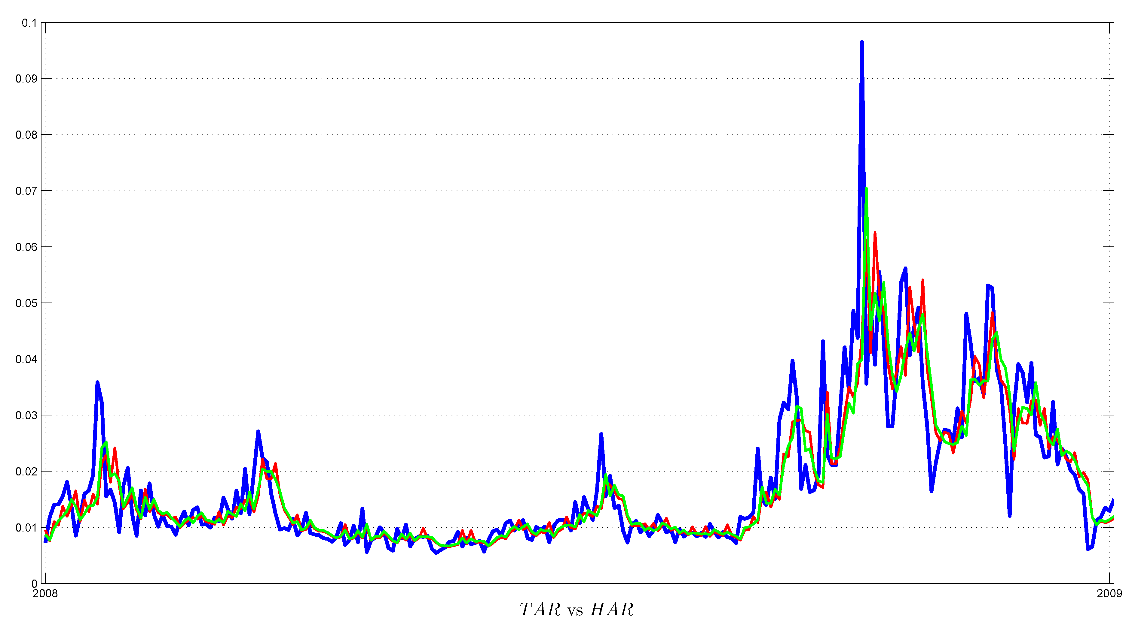
Finally, we assess the performance of volatility forecasts during times of financial turmoil: the U.S. financial crises in 2008 and the Eurozone crises in 2011. Although high-frequency models continue to dominate GARCH specifications, the benefits of using the non-linear TAR(2) model become substantial compared to linear specification: the latter’s MAE is higher by 3% (U.S. crises) and 6% (Eurozone crises). By contrast, the MAE of the HAR model is only 1% higher during the whole out-of-sample period. Figure 7 shows that TAR(2) better captures spikes in volatility than linear specification during the recent U.S. financial crises. Finally, both RMSE and MAE are lower for Eurozone crises and whole out-of-sample periods compared with recent U.S. financial crises, which reflects the learning process of the model, where recent volatility spikes help to improve the models’ performance.
To sum up, the benefits of using the non-linear TAR(2) model are most evident during periods of elevated volatility. In addition, the model is able to predict spikes in volatility, even when we use a relatively calm period for in-sample estimation, since changes in regimes are driven by moderately low returns. As a result, we do not rely on extreme market events to forecast volatility.
Figure 7.
Comparison of actual and one-day-ahead forecasts based on the TAR(2) and HAR models during U.S. financial crises from January 2008 to January 2009 (247 observations). Red and green lines indicate one-step forecasts based on the TAR(2) and HAR models, correspondingly, while the blue line the actual data.

4.2. Multiple-Step-Ahead Forecast
This section describes multiple-step-ahead forecasts for aggregate volatility. Specifically, the object of interests is the h-step forecast of aggregate realized volatility . Table 6 compares TAR(2) and other benchmark models during recent U.S. financial crises, Eurozone crisis and the out-of-sample period in 2008–2014. Figure 8 plots five-step-ahead forecasts for all models.
The main findings remain similar to the one-step-ahead forecasts. First, high-frequency models continue to dominate daily models at the five and 10 days’ ahead forecast. Second, TAR(2) performs better than the linear HAR model according to RMSE, MAE and . More importantly, the non-linear model outperforms linear specification, not only in a particular sample, but also in population: we reject the null hypothesis of the GW test that two forecast are identical at the 5% significance level. We based our conclusion on the results of the GW test for the 2008–2014 years to take into account the growing size of the out-of-sample dataset, as discussed in the Section 4.1. The GW test is based on the MAE metric. In addition, the U.S. financial crises have substantially higher RMSE and MAE compared with other periods, since periods of elevated volatility allow one to produce more accurate forecasts.
Finally, we compare TAR(2) and its competitors during recent financial crisis. The improvement in the MAE and RMSE metrics is comparable for crisis and longer out-of-sample periods and equal to approximately 2%. Although the GW test indicates that the TAR(2) and HAR model have the same forecasting errors, this can be explained by the relatively short size of the out-of-sample for both U.S. and Eurozone crises.
| TAR | HAR | GARCH | GJR | TAR | HAR | GARCH | GJR | TAR | HAR | GARCH | GJR | |
| 5-days-ahead forecast | ||||||||||||
| RMSE | 33.5 | 0.98 | 0.56 | 0.55 | 23.1 | 0.99 | 0.60 | 0.59 | 17.3 | 0.99 | 0.53 | 0.55 |
| MAE | 22.2 | 0.98 | 0.49 | 0.47 | 14.5 | 0.96 | 0.46 | 0.45 | 10.1 | 0.98 | 0.43 | 0.44 |
| R2 | 0.67 | 0.67 | 0.61 | 0.64 | 0.27 | 0.26 | 0.16 | 0.20 | 0.76 | 0.75 | 0.71 | 0.75 |
| pGW | NA | 0.13 | 0.00 | 0.00 | NA | 0.06 | 0.00 | 0.00 | NA | 0.03 | 0.00 | 0.00 |
| 10-days-ahead forecast | ||||||||||||
| RMSE | 69.2 | 0.98 | 0.48 | 0.48 | 47.6 | 0.98 | 0.50 | 0.50 | 35.2 | 0.98 | 0.44 | 0.45 |
| MAE | 47.0 | 0.97 | 0.41 | 0.40 | 30.6 | 0.96 | 0.36 | 0.35 | 20.6 | 0.97 | 0.33 | 0.33 |
| R2 | 0.63 | 0.63 | 0.61 | 0.61 | 0.15 | 0.15 | 0.16 | 0.14 | 0.73 | 0.73 | 0.71 | 0.74 |
| pGW | NA | 0.21 | 0.00 | 0.00 | NA | 0.31 | 0.00 | 0.00 | NA | 0.01 | 0.00 | 0.00 |
The first four columns correspond to the period of recent financial crises in the U.S. from January 2008 to January 2009 (247 observations). The next four columns correspond to Eurozone crises from July 2011 to December 2011 (123 observations). The last four columns correspond to the period from January 2008 to June 2014 (1604 observations). The performance metrics are the root mean square error (RMSE), mean absolute error (MAE), the of the Mincer–Zarnowitz regression and the p-value of the Giacomini and White test based on the MAE metric. Two forecasts are identical in population under the null hypothesis, while TAR beats its competitors under the alternative. The TAR column represents the actual value of RMSE and MAE errors, while the HAR, GARCH and GJR columns, corresponding to the RMSE and MAE rows, equal the ratio of TAR model to the following benchmark. Thus, a number below one indicates the improvement of the TAR model over its competitor. Observations for RMSE and MAE of the TAR model are standardized by 1000. Finally, the first four rows correspond to the 5-step-ahead, while the next four to the 10-step-ahead forecast, respectively. Observations from RMSE and MAE are standardized by 1000.
Figure 8.
Comparison of aggregate volatility over five days and corresponding forecasts based on the TAR(2), HAR, GARCH(1,1) and GJR-GARCH(1,1) models from January 2008 to June 2014 (1604 observations). The red line indicates the aggregate five-step forecast, while the blue line the actual data.
Figure 8.
Comparison of aggregate volatility over five days and corresponding forecasts based on the TAR(2), HAR, GARCH(1,1) and GJR-GARCH(1,1) models from January 2008 to June 2014 (1604 observations). The red line indicates the aggregate five-step forecast, while the blue line the actual data.

To sum up, our non-linear model outperforms its competitors thanks to its ability to capture different regimes in volatility and to measure volatility much more accurately than daily models. In addition, our model achieves approximately the same rate of improvement over the HAR model as much more complicated non-liner models, but with lower computational costs, since the TAR(2) model has only two regimes. For example, [18] modelled realized volatility with five regimes and achieved an improvement in forecasting performance over the HAR model of around 3%. This feature is essential for practical applications.
5. Conclusions
This paper develops a non-linear threshold model for RV (realized volatility), allowing us to obtain a more accurate volatility forecast, especially during periods of financial crisis. The changes in volatility regimes are driven by negative past returns, where the threshold equals approximately −1%. This finding remains robust to different functional forms of volatility and different set of indices from both developing and developed countries. The additional flexibility of the model allows one to produce a more accurate one-day-ahead forecast compared to the linear HAR specification and GARCH family models. More importantly, the superior multiple-step-ahead forecasting performance of TAR is achieved not only in particular samples, but also in population according to the GW test for the out-of-sample period from 2008 to 2014. Finally, we derive a closed form solution for multiple-step-ahead forecast, which is based on the NIG conditional distribution of returns. The non-linear threshold model primarily outperforms its competitors during periods of financial crisis.
The superior forecasting performance of TAR over other high-frequency models, as well as inter-daily GARCH specifications might warrant further examination. First, while the option pricing literature primarily relies on GARCH-type models, very few works exploit the availability of high-frequency data (e.g., see [40,46,47]). Thus, it might be useful to incorporate the TAR model into the option pricing framework, especially during periods of elevated volatility. We conjecture that a more accurate volatility model should result in lower hedging costs and, therefore, produce economic gains.
Second, the extension of the univariate to the multivariate models remains an important area of research given significant demand from practitioners. However, non-synchronicity is the key problem of estimating the covariance matrix despite the abundance of high-frequency data. Alternatively, a copula-based approach allows one to avoid this problem and to estimate the joint distribution of many assets. It would be interesting to incorporate the non-linear TAR model into the copula framework, since the current literature focuses either on the GARCH or HAR models ([48] and [49]).
Finally, the present work assumes that the diffusion process is continuous and, therefore, leaves the discussion of the jump process for further research.
Acknowledgements
The author thanks the three anonymous referees and editors, as well as John Knight, Lars Stentoft, Galyna Grynkiv, Miguel Cardoso, Juri Marcucci, Alex Maynard and Lynda Khalaf for their valuable comments and discussion. He also thanks the participants at the Midwest Finance Association 2015 Annual Meeting and Third Annual Doctoral Workshop in Applied Econometrics.
Appendix A
First, the GARCH(1,1) model is defined as:
The m-step-ahead forecast is computed according to:
Second, the GJR-GARCH(1,1) model is defined as:
The recursive formula for the multiple-step-ahead forecast of the GJR-GARCH(1,1) model is calculated as:
Appendix B
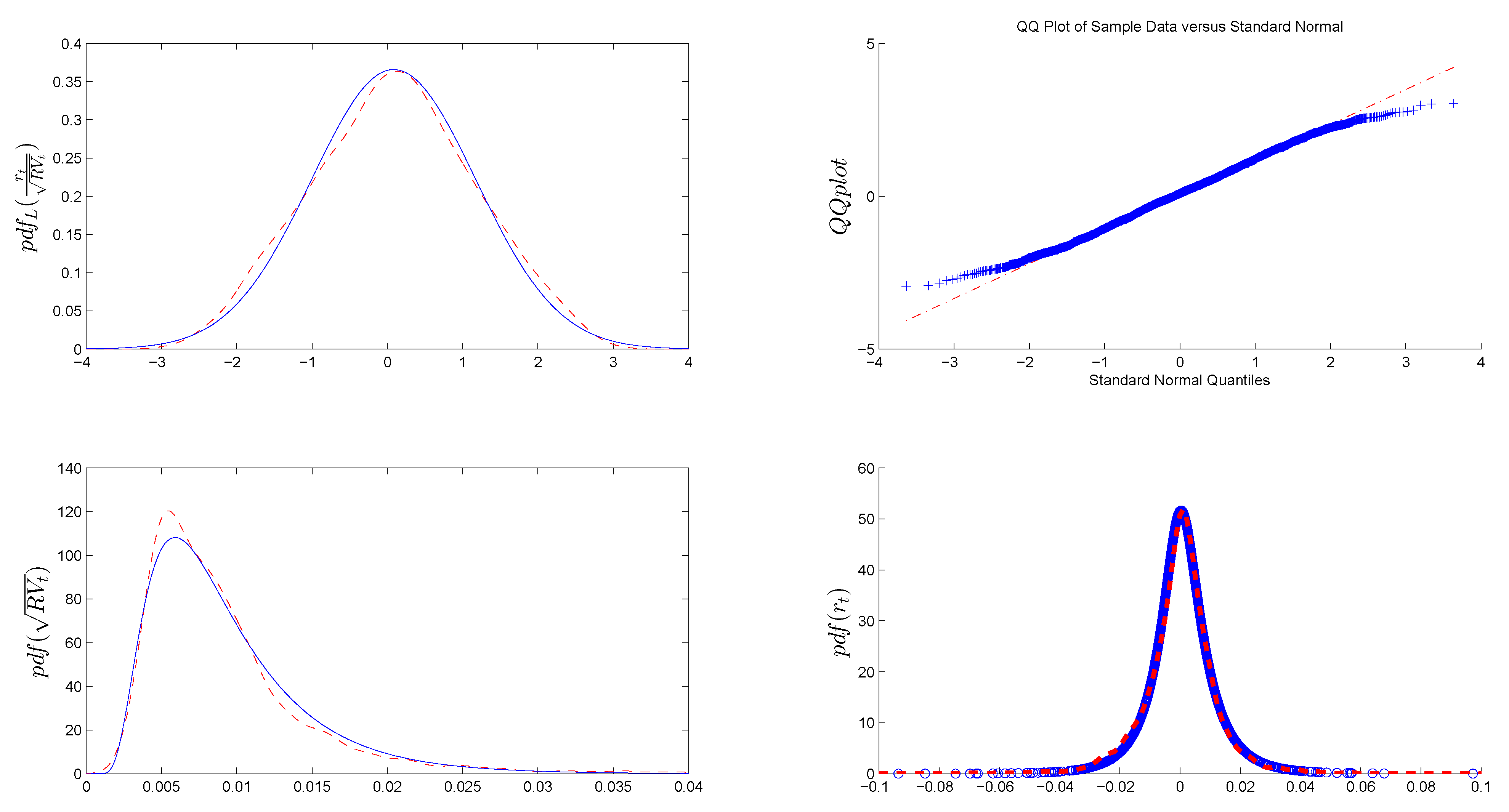
The first three graphs in Figure B1 demonstrate the very close match between parametric and non-parametric unconditional distributions of standardized returns and realized volatility, respectively. Table B1 shows the corresponding parameters of normal and inverse Gaussian distributions.
Table B1.
Parameters of normal and inverse Gaussian distributions for standardized returns and volatility.
| Parameters | All Sample | In-Sample |
|---|---|---|
| 0.0840 | 0.0488 | |
| 1.0907 | 1.0937 | |
| 0.0093 | 0.0087 | |
| 0.0296 | 0.0369 |
The first column corresponds to the in-sample period, while the second to the whole sample. is a scale parameter for the unconditional inverse Gaussian (IG) distribution of realized volatility.
Figure B1.
Comparison of parametric (solid blue line) and non-parametric kernel distributions (red dashed line) of standardized returns, realized volatility and returns. The first graph compares the normal distribution of standardized returns with the non-parametric distribution, while the second plots the corresponding QQ plot. The third graph illustrates the comparison between the IG distribution and the non-parametric distribution for realized volatility. The final graph shows the normal-inverse Gaussian (NIG) distribution for returns and the corresponding non-parametric distribution.

Appendix C
Proof of Theorem 1.
Recall that process is described as:
where and . The one-step-ahead forecast is obtained as:
Next, consider the the-step-ahead forecast from Equation (9):
Simplifying the first summand , we obtain:
Thus, Expression (C3) can be simplified as follows:
Using , Expression (C4) becomes:
where is . Finally, the formula for the multiple-step-ahead forecast with is extended recursively from Result (C5).
Conflicts of Interest
The author declares no conflict of interest.
References
- R. Engle. “Autoregressive Conditional Heteroskedasticity With Estimates of the Variance of UK. Inflation.” Econometrica 50 (1982): 987–1008. [Google Scholar] [CrossRef]
- T. Bollerslev. “Generalized Autoregressive Conditional Heteroskedasticity.” J. Econom. 31 (1986): 307–327. [Google Scholar] [CrossRef]
- T. Bollerslev, R. Engle, and D. Nelson. “ARCH Models.” In Handbook of Econometrics, Vol.IV. Edited by R. Engle and D. McFadden. Amsterdam, The Netherlands: Elsevier Science B.V., 1994, Chapter 49; pp. 2959–3038. [Google Scholar]
- J. Hull, and A. White. “The Pricing of Options on Assets with Stochastic Volatilities.” J. Financ. 42 (1987): 281–300. [Google Scholar] [CrossRef]
- A. Melino, and S. Turnbull. “Pricing Foreign Currency Options with Stochastic Volatility.” J. Econom. 45 (1990): 239–265. [Google Scholar] [CrossRef]
- T. Andersen, T. Bollerslev, F. Diebold, and P. Labys. “Modeling and Forecasting Realized Volatility.” Econometrica 71 (2003): 579–625. [Google Scholar] [CrossRef]
- J. Maheu, and T. McCurdy. “Do High-frequency Measures of Volatility Improve Forecasts of Return Distributions? ” J. Econom. 160 (2011): 69–76. [Google Scholar] [CrossRef]
- T. Andersen, T. Bollerslev, and F. Diebold. “Roughing it Up: Disentangling Continuous and Jump Components in Measuring, Modeling and Forecasting Asset Return Volatility.” Rev. Econ. Stat. 89 (2007): 701–720. [Google Scholar] [CrossRef]
- M. McAleer, and M. Medeiros. “A multiple regime smooth transition heterogeneous autoregressive model for long memory and asymmetries.” J. Econom. 147 (2008): 104–119. [Google Scholar] [CrossRef]
- T. Andersen, T. Bollerslev, F. Diebold, and H. Ebens. “The Distribution of Realized Stock Return Volatility.” J. Financ. Econ. 61 (2001): 43–76. [Google Scholar] [CrossRef]
- T. Andersen, and T. Bollerslev. “Heterogeneous Information Arrivals and Return Volatility Dynamics: Uncovering the Long-Run in High Frequency Returns.” J. Financ. 52 (1997): 975–1005. [Google Scholar] [CrossRef]
- C. Granger, and A. Ding. “Varieties of Long Memory Models.” J. Econom. 73 (1996): 61–77. [Google Scholar] [CrossRef]
- P. Perron. “The Great Crash, the Oil Price Shock and the Unit Root Hypothesis.” Econometrica 57 (1989): 1361–1401. [Google Scholar] [CrossRef]
- E. Zivot, and D. Andrews. “Further Evidence on the Great Crash, the Oil-Price Shock, and the Unit-Root Hypothesis.” J. Bus. Econ. Stat. Am. Stat. Assoc. 10 (1992): 251–270. [Google Scholar]
- K. Choi, W. Yu, and E. Zivot. “Long Memory versus Structural Breaks in Modeling and Forecasting Realized Volatility.” J. Int. Money Financ. 29 (2010): 857–875. [Google Scholar] [CrossRef]
- F. Corsi. “A Simple Approximate Long-Memory Model of Realized Volatility.” J. Financ. Econom. 7 (2009): 174–196. [Google Scholar] [CrossRef]
- R. Giacomini, and H. White. “Tests of Conditional Predictive Ability.” Econometrica 74 (2006): 1545–1578. [Google Scholar] [CrossRef]
- M. Scharth, and M. Medeiros. “Asymmetric effects and long memory in the volatility of Dow Jones stocks.” Int. J. Forecast. 25 (2009): 304–327. [Google Scholar] [CrossRef]
- O. Barndorff-Nielsen, and N. Shephard. “Econometric analysis of realized volatility and its use in estimating stochastic volatility models.” J. R. Stat. Soc. 64 (2002): 253–280. [Google Scholar] [CrossRef]
- O. Barndorff-Nielsen, and N. Shephard. “Estimating quadratic variation using realized variance.” J. Appl. Econom. 17 (2002): 457–477. [Google Scholar] [CrossRef]
- O. Barndorff-Nielsen, P. Hansen, A. Lunde, and N. Shephard. “Designing realised kernels to measure the ex-post variation of equity prices in the presence of noise.” Econometrica 76 (2008): 1481–1536. [Google Scholar] [CrossRef]
- C. Brownlees, and G. Gallo. “Comparison of volatility measures: A risk management perspective.” J. Financ. Econ. 8 (2009): 29–56. [Google Scholar] [CrossRef]
- U. Muller, M. Dacorogna, R. Dav, R. Olsen, O. Pictet, and J. Ward. “Fractals and Intrinsic Time—A Challenge to Econometricians.” In Proceedings of the XXXIXth International AEA Conference on Real Time Econometrics, Luxembourg, 14–15 October, 1993.
- H. Tong. “On a Threshold Model.” In Pattern Recognition and Signal Processing. Edited by C. Chen. Amsterdam, The Netherlands: Sijthoff and Noordhoff, 1978, pp. 101–141. [Google Scholar]
- H. Tong, and K. Lim. “Threshold Autoregression, Limit Cycles and Cyclical Data.” J. R. Stat. Soc. Ser. B Methodol. 42 (1980): 245–292. [Google Scholar]
- B. Hansen. “Testing for Linearity.” J. Econ. Surv. 13 (1999): 551–576. [Google Scholar] [CrossRef]
- R. Davies. “Hypothesis Testing When a Nuisance Parameter is Present Only Under the Alternative.” Biometrika 64 (1977): 247–254. [Google Scholar] [CrossRef]
- R. Davies. “Hypothesis Testing When a Nuisance Parameter is Present Only Under the Alternative.” Biometrika 74 (1987): 33–43. [Google Scholar]
- B. Hansen. “Sample splitting and threshold estimation.” Econometrica 68 (2000): 575–603. [Google Scholar] [CrossRef]
- F. Diebold, and C. Chen. “Testing structural stability with endogenous breakpoint. A size comparison of analytic and bootstrap procedures.” J. Econom. 70 (1996): 221–241. [Google Scholar]
- D. Andrews. “Tests for parameter instability and structural change with unknown change point.” Econometrica 61 (1993): 821–856. [Google Scholar] [CrossRef]
- F. Corsi, S. Mittnik, C. Pigorsch, and U. Pigorsch. “The volatility of realized volatility.” Econom. Rev. 27 (2008): 46–78. [Google Scholar] [CrossRef]
- K. Chan. “Consistency and Limiting Distribution of the Least Squares Estimator of a Threshold Autoregressive Model.” Ann. Stat. 21 (1993): 520–533. [Google Scholar] [CrossRef]
- B. Hansen. “Inference in TAR models.” Stud. Nonlinear Dyn. Econom. 2 (1997): 1–14. [Google Scholar] [CrossRef]
- P. Franses, and D. Dijk. Non-Linear Time Series Models in Empirical Finance. Cambridge, UK: Cambridge University Press, 2000. [Google Scholar]
- K. Chan, J. Petrucelli, and H.T.S. Woolford. “A multiple threshold AR(1) model.” J. Appl. Probab. 22 (1985): 267–279. [Google Scholar] [CrossRef]
- J. Knight, and S. Satchell. “Some New Results for Threshold AR(1) Models.” J. Time Ser. Econom. 3 (2011): 1–42. [Google Scholar] [CrossRef]
- L. Glosten, R. Jagannathan, and D. Runkle. “On the Relation between the Expected Value and the Volatility of the Nominal Excess Return on Stocks.” J. Financ. 48 (1993): 1779–1801. [Google Scholar] [CrossRef]
- L. Forsberg, and T. Bollerslev. “Bridging the Gap Between the Distribution of Realized (ECU) Volatility and ARCH Modeling (of the Euro): The GARCH-NIG Model.” J. Appl. Econ. 17 (2002): 535–548. [Google Scholar] [CrossRef]
- L. Stentoft. Option Pricing Using Realized Volatility. Aarhus, Denmark: CREATES Research Paper, 2008. [Google Scholar]
- G. Heber, A. Lunde, N. Shephard, and K. Sheppard. “Oxford-Man Institute’s realized library, Library version: 0.2.” Oxford, UK: Oxford-Man Institute, 2009. [Google Scholar]
- T. Andersen, T. Bollerslev, P. Frederiksen, and M. Nielsen. “Continuous-time models, realized volatilities, and testable distributional implications for daily stock returns.” J. Appl. Econom. 25 (2010): 233–261. [Google Scholar] [CrossRef]
- R. Dacco, and S. Satchell. “Why do Regime-switching Models Forecast so Badly? ” J. Forecast. 18 (1999): 1–16. [Google Scholar] [CrossRef]
- C. Ornthanalai. “Levy jump risk: Evidence from options and returns.” J. Financ. Econom. 112 (2014): 69–90. [Google Scholar] [CrossRef]
- P. Hansen, and A. Lunde. “A forecast comparison of volatility models: Does anything beat a GARCH(1,1)? ” J. Appl. Econom. 20 (2005): 873–889. [Google Scholar] [CrossRef]
- F. Corsi, N. Fusari, and D. Vecchia. “Realizing smiles: Pricing options with realized volatility.” J. Financ. Econ. 107 (2013): 284–304. [Google Scholar] [CrossRef]
- P. Christoffersen, B. Feunou, K. Jacobs, and N. Meddahi. “The Economic Value of Realized Volatility: Using High-Frequency Returns for Option Valuation.” J. Financ. Quant. Anal. 49 (2014): 663–697. [Google Scholar] [CrossRef]
- A. Patton, and I. Salvatierra. “Dynamic Copula Models and High Frequency Data.” J. Empir. Financ. 30 (2015): 120–135. [Google Scholar]
- D. Oh, and A. Patton. “High Dimension Copula-Based Distributions with Mixed Frequency Data.” J. Econom., 2015. Forthcoming. [Google Scholar]
© 2015 by the author; licensee MDPI, Basel, Switzerland. This article is an open access article distributed under the terms and conditions of the Creative Commons Attribution license (http://creativecommons.org/licenses/by/4.0/).
Share and Cite
MDPI and ACS Style
Pypko, S. Volatility Forecast in Crises and Expansions. J. Risk Financial Manag. 2015, 8, 311-336. https://doi.org/10.3390/jrfm8030311
AMA Style
Pypko S. Volatility Forecast in Crises and Expansions. Journal of Risk and Financial Management. 2015; 8(3):311-336. https://doi.org/10.3390/jrfm8030311
Chicago/Turabian StylePypko, Sergii. 2015. "Volatility Forecast in Crises and Expansions" Journal of Risk and Financial Management 8, no. 3: 311-336. https://doi.org/10.3390/jrfm8030311