Application of Vine Copulas to Credit Portfolio Risk Modeling

Abstract

In this paper, we demonstrate the superiority of vine copulas over conventional copulas when modeling the dependence structure of a credit portfolio. We show statistical and economic implications of replacing conventional copulas by vine copulas for a subportfolio of the Euro Stoxx 50 and the S&P 500 companies, respectively. Our study includes D-vines and R-vines where the bivariate building blocks are chosen from the Gaussian, the t and the Clayton family. Our findings are (i) the conventional Gauss copula is deficient in modeling the dependence structure of a credit portfolio and economic capital is seriously underestimated; (ii) D-vine structures offer a better statistical fit to the data than classical copulas, but underestimate economic capital compared to R-vines; (iii) when mixing different copula families in an R-vine structure, the best statistical fit to the data can be achieved which corresponds to the most reliable estimate for economic capital.

1. Introduction

From a methodological viewpoint, a misconception of credit portfolio risk was a core reason for the financial crisis of 2007–2008 (In particular, valuation of credit debt obligations (CDOs) is to a large extent based on measuring the credit portfolio risk of the underlying pool of loans. For an overview of CDO-related write-downs at major financial institutions, see [1]. An analysis of the crisis in a wider scope can be found in [2] or [3]). Modeling the correlation structure of a credit portfolio is mainly based on the Gaussian copula, which has received much criticism even in a non-academic context, see [4]. Against the background of this criticism, we introduce vine copulas (also referred to as pair-copula constructions) to the field of credit portfolio risk modeling and show that vine copulas are superior to conventional copulas. Since we dem

Conventional copulas exhibit particularly two shortcomings. First, in dimensions higher than two, the number of applicable copula families is restricted to the elliptical case and the Archimedean case; second, only simple, symmetric and therefore unrealistic dependence structures can be modeled. By decomposing a multivariate density into a cascade of conditional bivariate copulas, vine copulas circumvent these problems. There are numerous bivariate copula families with different properties that serve as building blocks for vine copulas, see [5,6]. This variety of bivariate copulas is exploited to form a rich and powerful multivariate distribution class even in large dimensions, which can model asymmetric and complex dependence structures.

However, the flexibility of vine copulas comes with the disadvantage that there is an abundance of different structures to choose from and it is a priori not clear which one to use. Standard procedures to tackle this problem have been studied and evolved over the past (see [7], for instance). In our analysis, we show how these approaches can be applied in the credit portfolio risk context to provide a robust estimation of economic capital. In contrast to [8], we are not restricted to D-vines and allow for higher dimensions. For a comprehensive collection of research on vine copulas, we refer to [9] or [10].

Credit portfolio risk is mostly driven by two components, namely obligor-specific default risk and cross-obligor dependencies. To model the former, we apply a structural model, which originates in [11] and in which default happens when the asset value of a company falls below its liabilities (Alternative obligor-specific default risk models are reduced form (or intensity) models, see [12,13]. For a comparison of both model classes, see [14] or [15]. Most of the criticism of structural models concerns the accuracy of credit spread predictions, whereas the focus of this paper is on the correlation structure among borrowers.). The dependence structure of the portfolio, which is the main concern of this paper, is modeled with copula functions. An alternative concept to model the dependence structure are factor models, see [16] or [17]).

In this paper, we fit vine copulas and conventional copulas separately to monthly equity returns of a Euro Stoxx 50 and an S&P 500 portfolio. Inferring credit or default correlations from the equity market may seem problematic at a first glance. The classical Merton model motivates the use of asset values to calibrate credit correlations, but even this approach has its limitations, as pointed out by [18]. Furthermore, due to various problems concerning the accessibility of asset values, equity prices are widely used as a substitute. Many banks rely on equity data for the calibration of the dependence structure of their internal credit portfolio models. For example, the correlation structure of CreditMetrics is estimated via equity data (see [19]) and Hull and White [20], p. 19 note that “default correlation between two companies is often assumed to be the same as the correlation between their equity returns.” Thus, from a practical point of view, the use of equity returns is justified. In addition, equity returns are the most important variable in predicting defaults, which provides an empirical link between equity data and credit risk, see [21].

We study D-vines and R-vines in this paper. As bivariate building blocks, we use the Gaussian (no tail dependence), the Student-t (tail dependence) and the Clayton copula (lower, but not upper tail dependence). For the Clayton family, we include the rotated versions as well (90, 180 and 270 degrees). After having fitted traditional D-vines and R-vine copulas to the data, we calculate the economic capital of the corresponding credit portfolio and compare the three approaches from a statistical and from an economic perspective. Our findings are (i) classical Gauss and Clayton offer the worst statistical fit (as measured in Akaike’s information criterion, briefly AIC) to the data; the Gauss copula underestimates economic capital while the Clayton copula overestimates the economic capital; the classical t copula is the best choice among the traditional copulas, both from a statistical and economic perspective; (ii) D-vine structures offer a better statistical fit to the data than the classic copulas but underestimate economic capital compared to R-vines; (iii) when mixing different copula families in an R-vine structure, the best statistical fit to the data is achieved that corresponds to the most reliable estimate for economic capital.

The outline of this paper is as follows. Section 2 gives a short primer on pair copulas, whereas Section 3 summarizes our credit portfolio risk framework. Section 4 is dedicated to a simulation study dealing with the feasibility of our calibration concept. Finally, the empirical results are presented in Section 5, and Section 6 concludes the paper.

2. A Short Primer on Pair-Copulas Including Specification and Estimation

Loosely speaking, a copula function $C(u_1,\dots ,u_n)$ with copula density $c(u_1,\dots ,u_n)$ is a multivariate distribution function on ${\left[0,1\right]}^n$ with uniformly distributed margins (see [5,6] for a rigorous definition and comprehensive presentation of copulas). According to [22], any given multivariate distribution function F with density f can be expressed with the help of a copula function C as follows:

$$F\left(x\right)=C(F_1\left(x_1\right),\dots ,F_n\left(x_n\right)).$$

(1)

If the marginal distributions $F_i$ are continuous, the copula function C is unique. Provided its existence, c denotes the corresponding density. In contrast to the wide-spread class of elliptical copulas, our focus is on vine copulas henceforth (For a detailed treatment of multivariate copula models, we refer to [23] or [24], for instance). Vine copulas (Comprehensive contributions to vine copulas are provided by [25,26], [9] or [10]) are a flexible class of dependence models consisting of bivariate building blocks and have proven to be particularly useful in high dimensions. The origin of vine copulas dates back to [27], who describes how multivariate distributions can be sequentially decomposed into bivariate building blocks via conditioning. In order to give structure to these decompositions within a copula setting, so-called regular vines (briefly: R-vines) have been introduced by [28] that comprise the information about the factorization of the multivariate copula density function into the density functions of its pair copulas. In a very general sense, a vine on n variables is a set of $n-1$ trees in which the edges of tree $T_i$ become the nodes of the subsequent tree $T_{i+1}$. Regular vines have the additional property that two nodes in tree $T_{i+1}$ are connected by an edge if they share a common node in the previous tree $T_i$, which is called “proximity condition”. For $n=3$, one possible factorization of the copula density is

$$c(u_1,u_2,u_3)=c_{12}(u_1,u_2)·c_{13}(u_1,u_3)·c_{23\mid 1}(C_{2\mid 1}(u_2\mid u_1),C_{3\mid 1}(u_3\mid u_1)).$$

(2)

Aas et al. [29] illustrate a first application of the vine copulas applying non-Gaussian pair copulas to financial data. Apart from many applications to financial data like [30], pair-copula constructions are used in areas as diverse as hydrology, medicine or genetic and evolutionary computation, see [31,32,33], respectively. 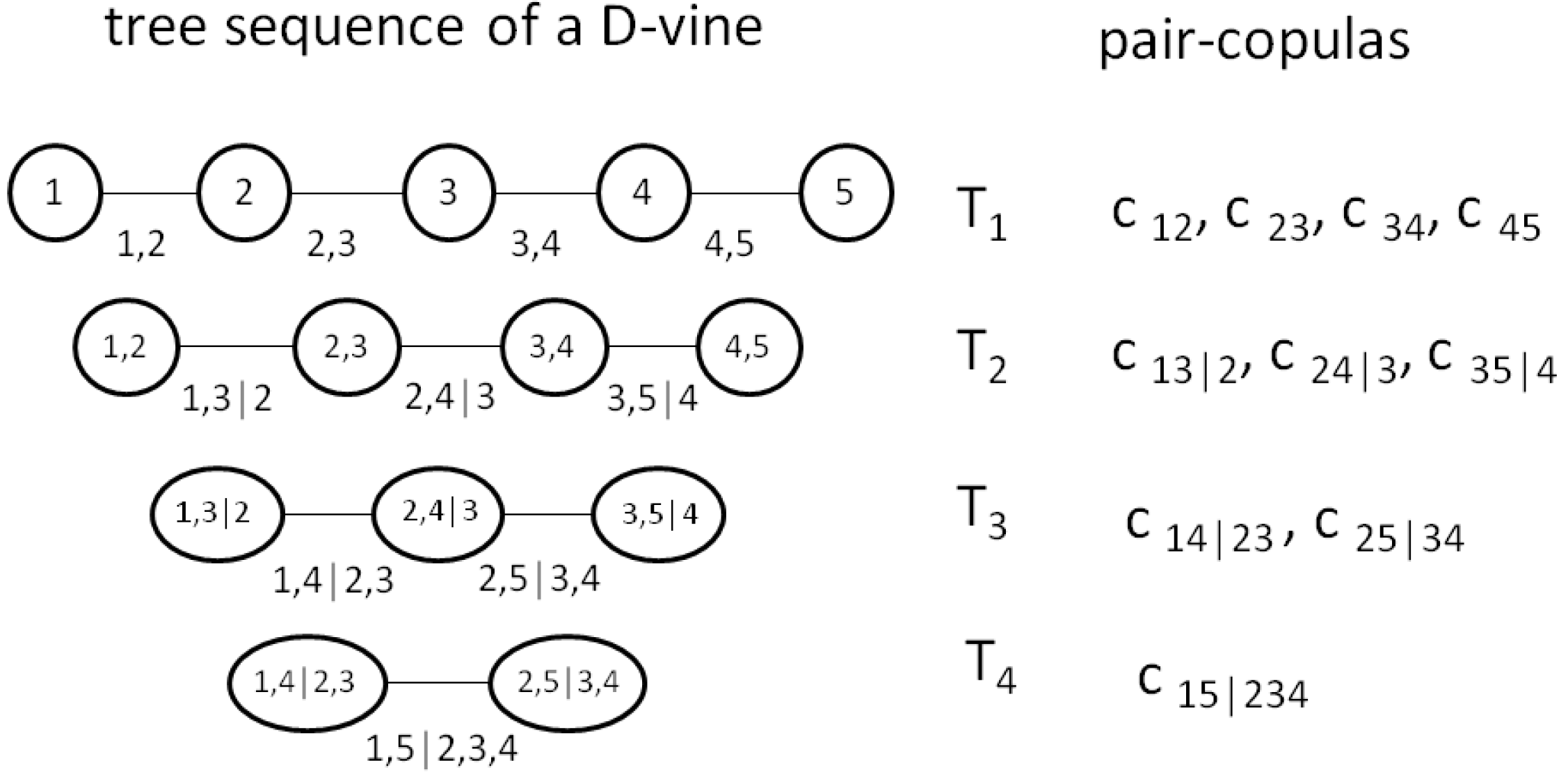Being still very comprehensive and containing a huge number of possible decompositions (see [34]), two popular subclasses—known as C-vines and D-vines—appeared in the subsequent literature. In a D-vine setting, all trees have a path-like structure, that is, any given node is not connected to more than two other nodes. Exemplarily, Figure 1 shows the set of trees with corresponding pair-copulas of a five-dimensional D-vine. Tree $T_1$ represents the unconditional bivariate copulas (see Equation (2)), while the remaining trees represent the remaining conditional copulas. In contrast, in a C-vine setting, all trees have star-shape structures—in every tree there is one node (the so-called pivot element) which is connected to all other nodes. Since in the credit portfolio context there is no economic reason to use a pivot element, our focus is on D-vine constructions.

Although the pair-copula decomposition is not unique, the major advantage of this approach is that the conditional bivariate copulas do not have to be from the same family but can be chosen freely from any kind of copula family. Consequently, very complex and asymmetric dependence structures can be modeled. The specific definition of pair-copulas leads to three fundamental estimation and selection tasks (see e.g., [35]): firstly, estimation of copula parameters for a chosen vine tree structure and pair copula families (for details on estimation of vine copulas like SSP or ML (maximum likelihood) estimation, we refer to [29,36,37,38] or [39]); secondly, selection of the parametric copula family for each pair copula term and estimation of the corresponding parameters for a chosen vine tree structure; and, thirdly, selection and estimation of all three model components.

In order to select the vine structure, two construction strategies have been proposed in the literature: a top-down approach by [7] and a bottom-up method by [38]. In our setting, the heuristic is to use the basis tree which captures the strongest dependencies as measured by pairwise Kendall’s τ, which means that in a D-vine we have to find pairs of variables and arrange them one after another so that the sum of the absolute pairwise Kendall’s τ is maximized. This problem corresponds to finding a Hamiltonian path with maximum weight in the complete graph in which the variables represent the vertices and the Kendall’s τ is the weight of the corresponding edge. For an R-vine, the approach of capturing the strongest dependencies in the ground-level tree is similar; however, no path like structure is needed but a maximum spanning tree (all variables are connected, but there are no circles). Finding maximum spanning trees and Hamiltonian paths are classic Operations Research problems and can be solved using standard algorithms. By considering other approaches for the basis tree selection, we checked that our results are robust to this heuristic.

As bivariate building blocks, we use the Gauss copula (no tail dependence), the t copula (tail dependence) and the Clayton copula (admits lower, but no upper tail dependence). Having fitted different vine copula models to a given data set, the best model in terms of the classical AIC is identified. Our analysis is done with the R-package CDVine from [40] for D-vines and on the R-package VineCopula [41] which is a continuation of the package CDVine.

3. Calculating Economic Capital Based on Copulas

In order to absorb unexpected losses of a loan portfolio, banks are required to retain economic capital. Typically, the amount of capital a bank has to hold is determined with a credit portfolio risk model. Very common industry models are CreditRisk${}^{+}$ by [42] and CreditPortfolioView from [43], and, as representatives of so-called structural model, CreditMetrics, see [19] and KMV (see [44]). In the context of structural models, the default of an obligor $i\in \{1\dots ,n\}$ occurs when its creditworthiness $B_i$ (treated as a latent variable) falls below a pre-specified threshold $d_i$, i.e., $B_i\le d_i$. Typically, the underlying time horizon within a credit portfolio risk context is one year, and the default threshold is calculated as $d_i={\Phi }^{-1}\left(P{D}_i\right)$, where $P{D}_i$ denotes the one-year probabilities of default for obligor i. It is an exogenous input parameter derived from the bank’s rating tool. In contrast to the classical setting, where $B=(B_1,...,B_n)$ are assumed to follow a multivariate Gaussian distribution, we assume that each marginal distribution $F_i\left(x_i\right)=P(B_i\le x_i)$ for $i=1,\dots ,n$ has a univariate Gaussian law, but the underlying copula C belongs to the pair-copula class, which allows for complex and asymmetric dependence structures. For a discussion of copulas in the context of CreditRisk+ and CreditMetrics, we refer to [45,46]. Hence, the loss distribution in our setting reads as

$$L=\sum _{i=1}^n{N}_i·1_{\left\{B_i\le d_i\right\}}\mathrm{with}{F}_B\left(x\right)=C(\Phi \left(x_1\right),\dots ,\Phi \left(x_N\right)),$$

(3)

where $N_i$ is the notional of the loan given to obligor i and $F_B$ denotes the multivariate distribution of the vector $B=(B_1,...,B_n)$. For reasons of clarity, the following assumptions are met: first, we abstract from the decomposition of $N_i$ the exposure at default and the loss given default and use a constant and deterministic $N_i$. In reality, exposure at default and loss given default are stochastic variables that have to be modeled, but since we are primarily interested in correlation issues, we streamline our analysis at this point. Second, losses due to rating migrations are not within the scope of our analysis. This facilitates getting the point across but does not affect the overall conclusion. Third, as mentioned above, the creditworthiness process relies on a plain geometric Brownian motion and is restricted to a one-year horizon. If more complex structures for the creditworthiness index are needed (which goes beyond the scope of this paper), for example a diffusion process with a constant volatility plus a jump, or a double-exponential jump-diffusion process, we refer the reader to [47] or [48].

In the end, the loss distribution is derived by Monte Carlo simulation, which is drawing multivariate samples $(B_1,\dots ,B_n)$ from the distribution function F and evaluating Equation (3). From the (empirical) distribution of the portfolio loss, L, one can derive risk figures like expected loss (EL), Value at Risk (VaR) or the corresponding economic capital which is commonly defined as VaR minus EL.

4. Simulation Experiments

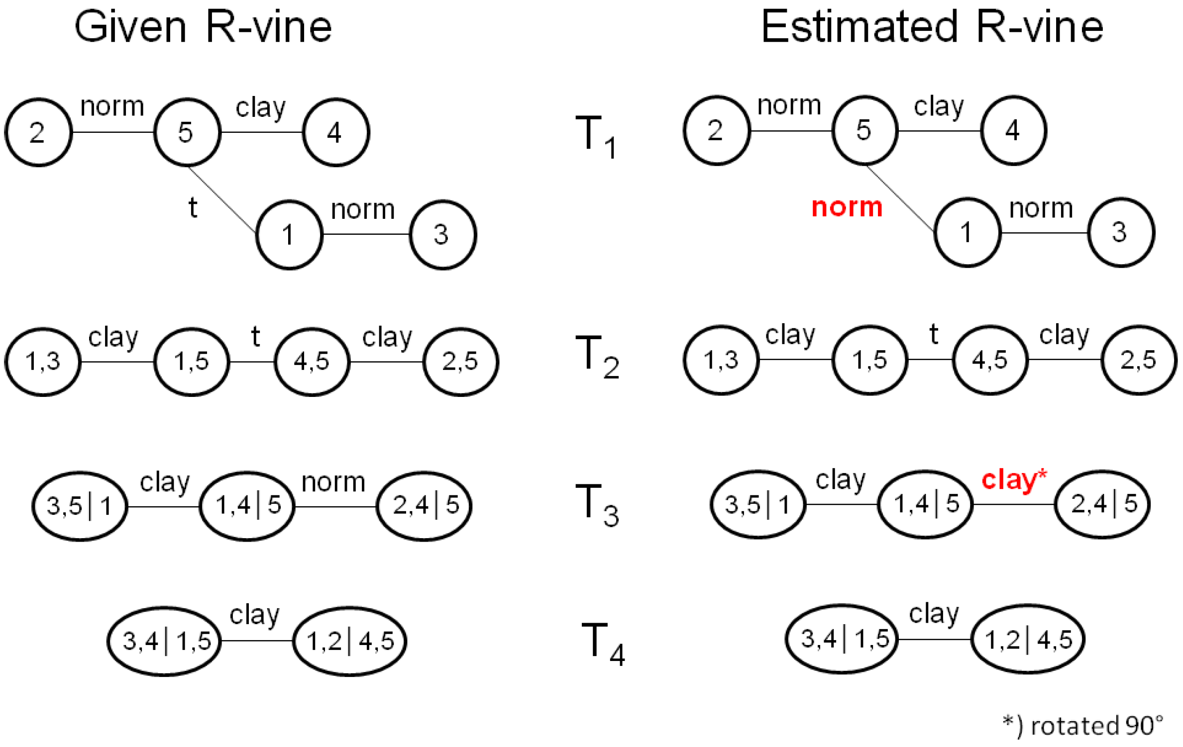
To check whether the vine copula calibration concept from Section 2 is feasible, we conduct a simulation experiment in which we sample from a known vine copula, apply the estimation approach to the sampled values and compare the known with the fitted vine copula. As in real life, the model user neither knows tree structure nor bivariate copula families nor bivariate copula parameters (bivariate copula families are a little exception in this regard as we restrict ourselves to the Gauss, t and Clayton family). Given the abundance of possible vine structures to sample from, we want our simulation experiment to mimic a realistic setting. Therefore, we choose five companies randomly from the Euro Stoxx 50, fit an R-vine to their equity time series and use the resulting R-vine as the known copula in the simulation experiment (chapter 5 will show that R-vines are superior to D-vines, which is why we restrict the simulation study to R-vines). By doing so, we ensure using a realistic tree structure with realistic copulas and parameters. It turns out that all three copula families are included in the known copula. We generate 150 samples from the known vine copula, as this a realistic number of observations. 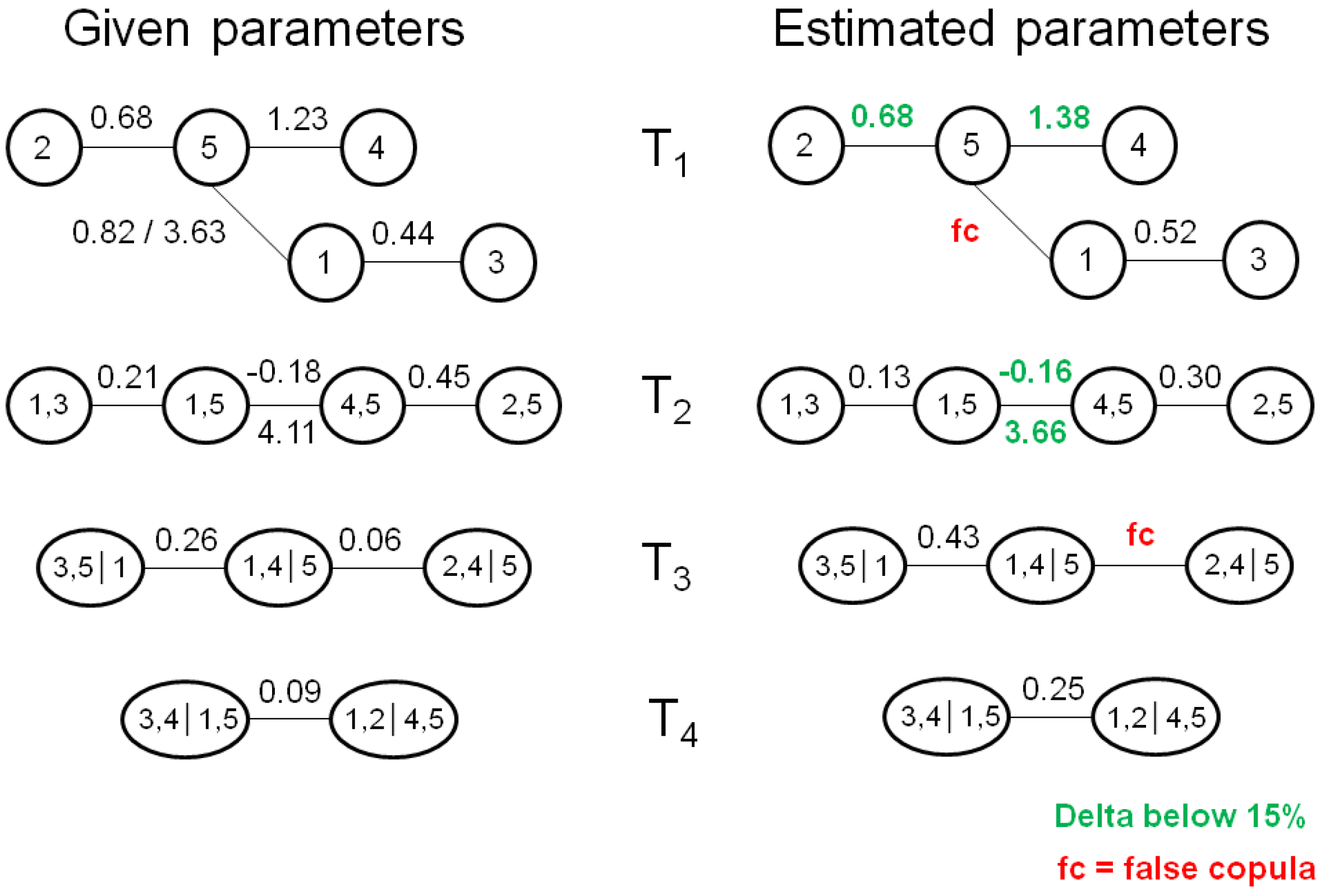The left side of Figure 2 shows the given vine structure from which we draw 150 samples, while the right side shows the vine structure which results from fitting an R-vine to the 150 observations. The estimated tree structure is identical to the given one, which is actually quite remarkable given that there are 480 different R-vines on five variables. In addition, the selected bivariate copula families are also pretty close to the known ones, as eight out of ten bivariate copula families are correctly estimated. Next, we compare the parameters of the bivariate copulas from the given copulas with the estimated ones (see Figure 3). Especially in the ground level trees, $T_1$ and $T_2$, the parameter match is rather good, while the deviations increase as we move to the top level trees. The largest parameter deviation appears for the top level tree, $T_4$, in which the real Clayton parameter is overestimated quite a bit (0.06 vs. 0.25). We highlighted parameter deviation of less than 15% in green.

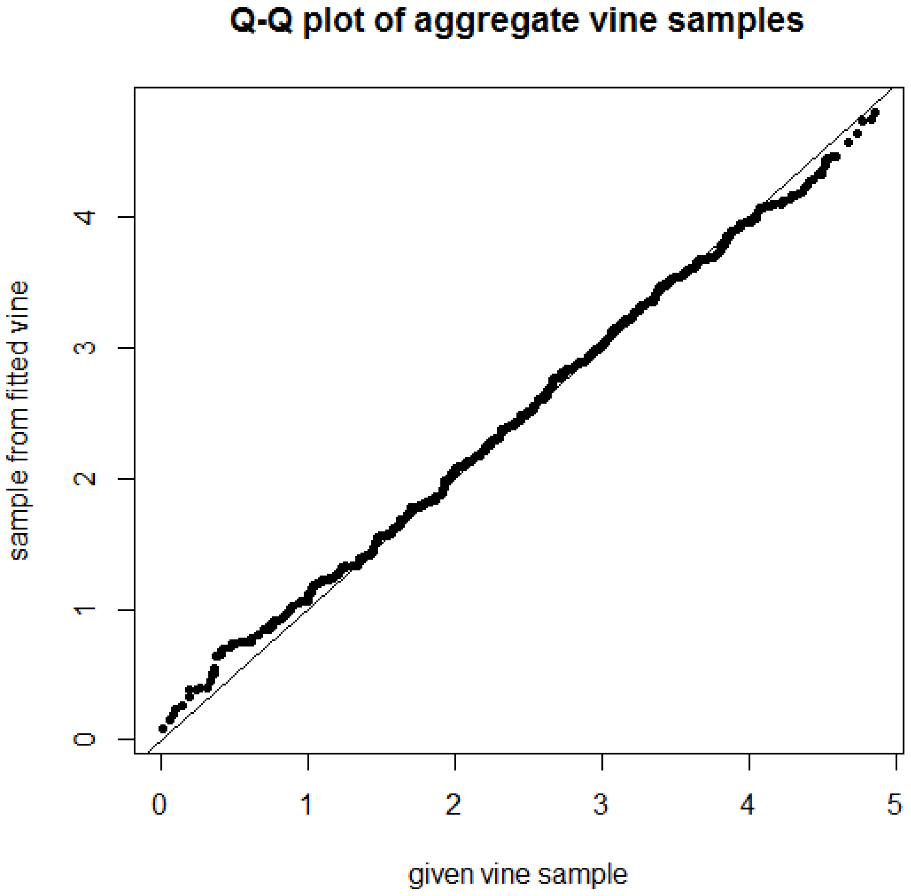
To judge the impact of the observed deviation in bivariate copula parameters on an overall level, we use a qq-plot. As we are concerned with credit portfolio risk modeling, it is the aggregate portfolio behavior which is more important to us than the behavior of a single creditor (provided that the portfolio is well diversified). The aggregate portfolio behavior can be described by summing up the entries of each five-dimensional vine sample to a single value, which we do for the 150 given vine samples. Next, we generate 150 vine samples from the fitted vine copula (see right side of Figure 2 and Figure 3) and calculate the aggregate values accordingly. Figure 4 plots the quantiles of the aggregate given vine sample against the quantiles of the aggregate sample from the fitted vine copula. On the aggregate portfolio level, the overall fit appears to be rather good, which implies that we can tolerate some deviations in bivariate copula parameters given that the selected tree structure and copula families are pretty good.

Two things are pretty obvious now. First, we cannot draw conclusions from a single simulation experiment, which is why we repeat the experiment described above many times. Second, an in-depth comparison of known to fitted vine copula as we did above (tree structure, bivariate families and copula parameters) cannot be performed on more than two or three simulation experiments, which is why we need a single metric to judge how ’close’ the fitted vine is to the known vine. For this end, we use the AIC ratio defined as:

$$\mathrm{AIC}\mathrm{ratio}=\frac{\mathrm{AIC}(\mathrm{fitted}\mathrm{vine},150\mathrm{observations})}{\mathrm{AIC}(\mathrm{known}\mathrm{vine},150\mathrm{observations})}.$$

(4)

The simulation experiment that we analyzed in detail in Figure 2, Figure 3 and Figure 4 has an AIC ratio of 104.4%, which serves as a reference point of interpreting AIC ratios.

As we want to study the impact of the number of observations N, we keep the copula dimension fixed at five and repeat our simulation experiment 50 times for $N=50$, $N=150$ and $N=500$ each.

Table 1. Impact of copula dimension and number of observation on estimation performance.

	Dimension = 5			N = 150
	N = 50	N = 150	N = 500	dim = 5	dim = 10	dim = 15
Average AIC ratio	131%	104%	99%	104%	104%	105%

This table shows AIC ratios averaged over 50 iterations for a different copula dimensions and numbers of observations.

, in which AIC ratios averaged over the 50 iterations are displayed, confirms what common sense suggests, i.e., with increasing number of observations, the estimation results get better. AIC ratio drops from 131% to close to 100% when N is increased from 50 to 500 (see left panel of Table 1). In particular, we see that the conclusion of the rather good fit from the simulation experiment of Figure 2, Figure 3 and Figure 4 can be generalized because the average AIC ratio of 50 iterations is pretty close to the AIC ratio of the single experiment (104% vs. 104.4%) for $N=150$. We can generalize our conclusion from the single simulation experiment that in dimension five, 150 observations are enough to get a pretty good estimation result.

As dimension five is clearly too low from a practitioner’s point of view, we have to analyze how the estimation results behave when the copula dimension increases. We do so by fixing the number of observations at $N=150$ and double and triple the dimension to $dim=10$ and $dim=15$ (see right panel of Table 1). Note that $N=150$ must not be mistaken for the absolute number of observations, but for the number of $dim$-dimensional observation vectors (e.g., in $dim=10$, we have a 10 × 150 observations matrix and 1500 observations in absolute terms).

Interestingly, the copula dimension hardly has any effect on estimation performance (which is quite comforting for our plan to use vine copulas in dimension 40 and 75). When the copula dimension is increased by a factor of three (from five to 15), the average AIC ratio hardly changes (from 104% to 105%). We can easily explain the estimation’s robustness towards the dimension by looking at the ground level trees of the vine: no matter what the dimension is, at each bivariate estimation step, there is a 150 × 2 observation matrix available to estimate the bivariate copula from. Obviously, the estimation results of the ground level trees do not deteriorate if we repeat the bivariate copula estimation with increasing dimension. The same argument holds for the higher level trees. Figure 5 presents boxplots of the 50 AIC ratios underlying each average value of Table 1. The boxplots support our conclusion that estimation performance increases with number of observations and that the copula dimensions have hardly any effect.

5. Applying Vine Copulas to a Credit Portfolio

To investigate the practical consequences of using vine copulas compared to conventional copulas, we consider a loan portfolio of 40 companies from the Euro Stoxx 50 and 75 companies from the S&P 500, respectively. In the case of the Euro Stoxx 50, the maximum number of companies for which the equity time series are available for the complete time period under investigation is 40. The 75 companies from the S&P 500 are drawn at random to increase the dimension and to perform some kind of robustness check. We fit the copulas to end-of-month equity log-returns from the time period from December 1999 to March 2011, which total 135 observations.

Table 2. Comparison of AIC for conventional and vine copulas.

	Euro Stoxx 50			S&P 500
	Classic	D-vine	R-vine	Classic	D-vine	R-vine
Gaussian	−2.880	−2.922	−2.922	−3.730	−3.738	−3.744
t	−3.184	−3.182	−2.995	−4.134	−3.006	−3.255
Clayton	−2.040	−3.024	−3.267	−2.580	−3.824	−4.255
flexible	-	−3.577	−3.688	-	−5.035	−5.616

AIC values of different copulas which have been fitted to equity time series of 40 companies from the Euro Stoxx 50 and 75 companies from the S&P 500.

presents the AIC for conventional copulas, D- and R-vines for both portfolios. The first three rows refer to vine copulas where all bivariate copula are taken from the family given in the very first column, whereas, in the flexible construction, the copula family with the highest AIC is chosen in each bivariate estimation step. Looking at the traditional copulas, we see that for both portfolios, the t copula clearly outperforms the Gaussian and the Clayton copula (e.g., Euro Stoxx: −3.184 vs.−2.880/−2.040), which is no big surprise given the inability of the Gauss copula to model tail dependence and given that the classical Clayton copula is pretty limited with only one parameter. When using D-vines instead of classical copulas, there is little effect on the AIC for the Gaussian (e.g., Euro Stoxx: −2.880 vs.−2.922), which is not surprising as the classical Gauss copula, D- and R-vines are mutually equivalent (Parameters of the pair-copulas in the vine structure equal the corresponding partial correlation coefficients of the conventional Gaussian copula, see [49], Section 2.7.4. In addition, the stepwise and the joint estimation are both asymptotically efficient in this case, which is showed in [36]). Differences in AIC are due to numerical maximum likelihood estimation issues. In the t copula case, the higher flexibility of D-vines is offset by the AIC punishment for number of parameters. For the S&P 500 portfolio, this effect is even more strongly pronounced than for the Euro Stoxx portfolio (−3.184 vs.−3.182 and −4.134 vs.−3.006). Only in the Clayton case is there a clear benefit of using a D-vine compared to the classical case. Interestingly, the ability to mix different families is needed for the D-vine to beat the classical t copula in both portfolios.

When using R-vines, the observation is pretty similar to the D-vine case: there is hardly any benefit of using R-vines in the Gaussian and t family, while for the Clayton case, the R-vine clearly beats the D-vine structure for both portfolios. Finally, we see that the flexible R-vine beats the flexible D-vine, whereas this effect is more pronounced in the S&P 500 portfolio (−5.035 vs.−5.616) than in the Euro Stoxx portfolio (−3.577 vs.−3.688).

The general conclusion from our calibration exercise is (i) the t copula is the best choice among the traditional copulas; (ii) the advantage of vine copulas does not come solely from the flexible tree structure, but the flexibility of mixing different bivariate families is used to beat the classical t copula and (iii) R-vines are better than D-vines (which is actually not too surprising given the higher flexibility in the tree structures).

Next, we turn to the economic implications of using vine copulas.

Table 3. Comparison of economic capital for conventional and vine copulas.

	Euro Stoxx 50			S&P 500
	Classic	D-vine	R-vine	Classic	D-vine	R-vine
Gaussian	15.8	-	-	18.4	-	-
t	24.6	20.1	24.7	32.4	26.3	33.0
Clayton	29.1	16.7	28.3	38.0	22.0	31.3
flexible	-	20.0	26.4	-	23.8	34.3

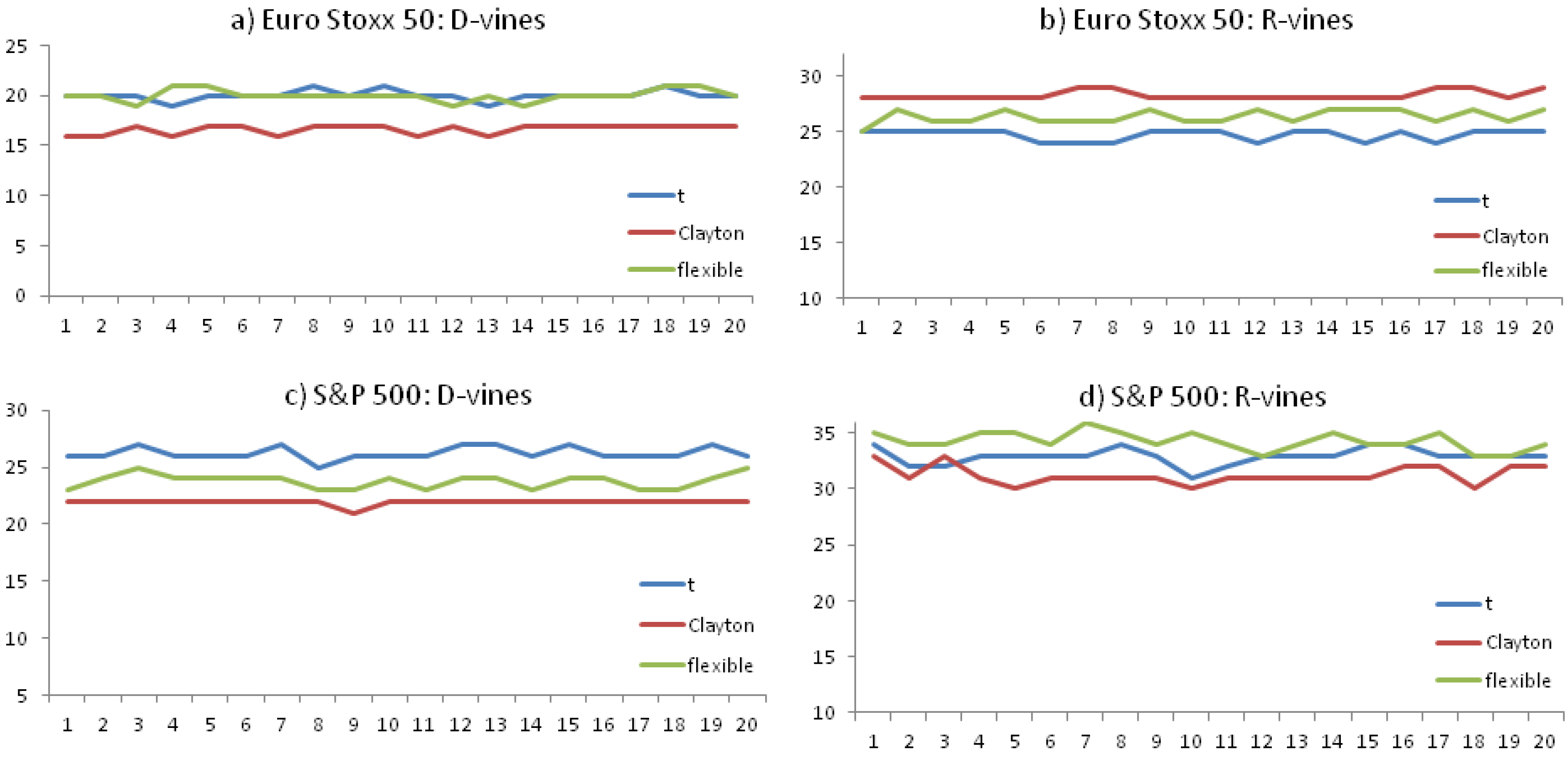
Portfolio consists of 40 and 75 borrowers, respectively, with constant $PD=1\%$. VaR (99.9%) is given as the average of 20 runs. Sample size for the portfolio loss distribution is 100,000.

displays economic capital values calculated based on the copulas from Table 2. Economic capital is calculated as the 99.9% quantile of the portfolio loss distribution, which, in turn, is calculated based on 100,000 copula samples. As we apply a constant PD and a constant exposure throughout the portfolio, the expected loss is constant and we refrain from subtracting the expected loss from the portfolio loss distribution quantile. We found that the 99.9% quantile at 100,000 iterations is pretty stable (for details, see Appendix A). Nevertheless, we report economic capital averaged over 20 runs in Table 3. We use a constant probability of default of 1% for all borrowers. Note that the variations in economic capital discussed below are exclusively due to changes of the copula, as the marginals are held fixed to be Gaussian. As noted above, there is no difference between classic, D- and R-vines in the Gaussian case, which is why we suppress economic capital values in the Gaussian D- and R-vine cases for concise presentation. The Gaussian copula comes up with the lowest economic capital value for both portfolios (15.8 and 18.4) among all copula specifications, while the classical Clayton comes up with the highest economic capital value (29.1 and 38.0) overall. This effect holds for both portfolios. Taking the rather low AIC value for classical Gauss and Clayton copula into account (see Table 2), we conclude that the classical Gaussian (Clayton) copula underestimates (overestimate) the economic capital. Compared to their traditional counterparts, D-vine copulas result in remarkably lower economic capital values, which holds for both portfolios (e.g., Euro Stoxx and Clayton: 29.1 vs. 16.7). Economic capital increases when D-vines are replaced by R-vines (e.g., S&P 500 and t: 26.3 vs. 33.0), which is an effect that holds also in the flexible case (e.g., Euro Stoxx: 20.0 vs. 26.4). Following the AIC ranking and choosing the flexible R-vine as the best model, we conclude that the best estimate for economic capital is 26.4 (Euro Stoxx) and 34.3 (S&P 500). Interestingly, all copula models deviate quite a bit from the best estimate of economic capital as proposed by the flexible R-vine model, which implies that there is a real benefit of using a flexible R-vine as it comes up with a unique risk estimation that cannot be replicated by other copula models. Maybe the only exception in this regard is the R-vine t copula coming closest for the S&P 500 portfolio (33.0 vs. 34.3) but having a clearly lower AIC score.

As the flexible R-vine is the best choice for modeling the correlation structure of a credit portfolio, we take a closer look at its composition and parameters.

Table 4. Flexible R-vine in detail.

	Euro Stoxx 50				S&P 500
	Selections	Mean θ	Min θ	Max θ	Selections	Mean θ	Min θ	Max θ
Gaussian	26%	0.04	−0.31	0.75	30%	0.04	−0.28	0.83
t (df)	11%	4.4	2.0	7.9	8%	5.2	2.0	11.3
t (corr)	-	0.24	−0.17	0.88	-	0.15	−0.27	0.78
Clayton	63%	0.24	0.01	2.17	62%	0.17	0.01	1.65

This table shows the composition of the flexible R-vine together with summary statistics of the estimated parameters.

shows that Clayton is the predominant family for both portfolios with 63% and 62% selections. For the remaining copulas, the Gaussian family is chosen more often than the t copula (e.g., Euro Stoxx: 26% vs. 11%). In addition, summary statistics of the estimated parameters are displayed that are rather robust across both portfolios.

Finally, two exercises related to backtesting. First, we wanted to study how our estimate for economic capital reacts towards a growing time series. Our time series used for the copula fitting stopped in March 2011, which included 135 observations. We repeated the copula calibration with time series that ended in January 2016, which included 194 observations (+42% observations). We restricted our analysis to the S&P 500 portfolio and a flexible R-vine (best fit) and the classical Gauss copula (rather worse fit, but most popular copula). Between March 2011 and January 2016, five companies left our sample due to merger or take-overs (not due to default), which is why we cannot take the original economic capital values of Table 3 as reference point for the analysis. We repeat the copula calibration based on time series ending in March 2011 for the portfolio without the five companies that left the sample, which is the new reference point for the analysis.

Table 5. Stability of S&P 500 economic capital figures.

	Up to March 2011	Up to January 2016
Gauss classic	16	18
R-vine flexible	28	29

This table shows how economic capital reacts when the time series used for calibration are extended from March 2011 until January 2016. The portfolio is reduced by five companies compared to Table 3, all other specifications are unchanged.

shows that, for both copula types, the estimate for economic capital is rather stable when the time series is extended from March 2011 to January 2016. In the Gaussian case, economic capital is increased from 16 to 18 defaults, whereas the increase for the flexible R-vine is somewhat lower (from 28 to 29). We conclude that the vine copula framework is quite stable towards a growing time series.

The second analysis is more related to backtesting in a classical sense. Classic backtesting, is comparing a given risk metric, which is derived from a risk model and which is a forecast about the future, with ex-post observations. For this purpose, there are two non-overlapping time frames. The first time frame (i.e., the training period) is used to calibrate the model. At the end of the training period, the risk metric as a prediction about the up-coming future is derived from the calibrated model. Then, the model user wants to know how accurate the model’s prediction about the future really is. Therefore, a backtesting period is defined (usually at the end of the training period) and the model user checks how the risk metric materializes in the backtesting period, and whether it is in line with the model’s prediction. If the risk metric in the backtesting period strongly deviates from what the model has predicted, there is a rather clear indication that something is wrong in the model set-up.

We transform these considerations to our model set-up in the following way: analogous to the first backtesting exercise above, we fix the training period as December 1999 to March 2011 and use the time from April 2011 to January 2016 as the backtesting period. We restrict our analysis again to the reduced S&P 500 portfolio from above and use a flexible R-vine and the classical Gauss copula. The risk metric to which we apply the backtesting is the portfolio loss distribution (where loss is measured in number of defaults). More specifically, we backtest the tail of the loss distribution because credit portfolio risk modeling is mostly concerned with the tails of the loss distribution.

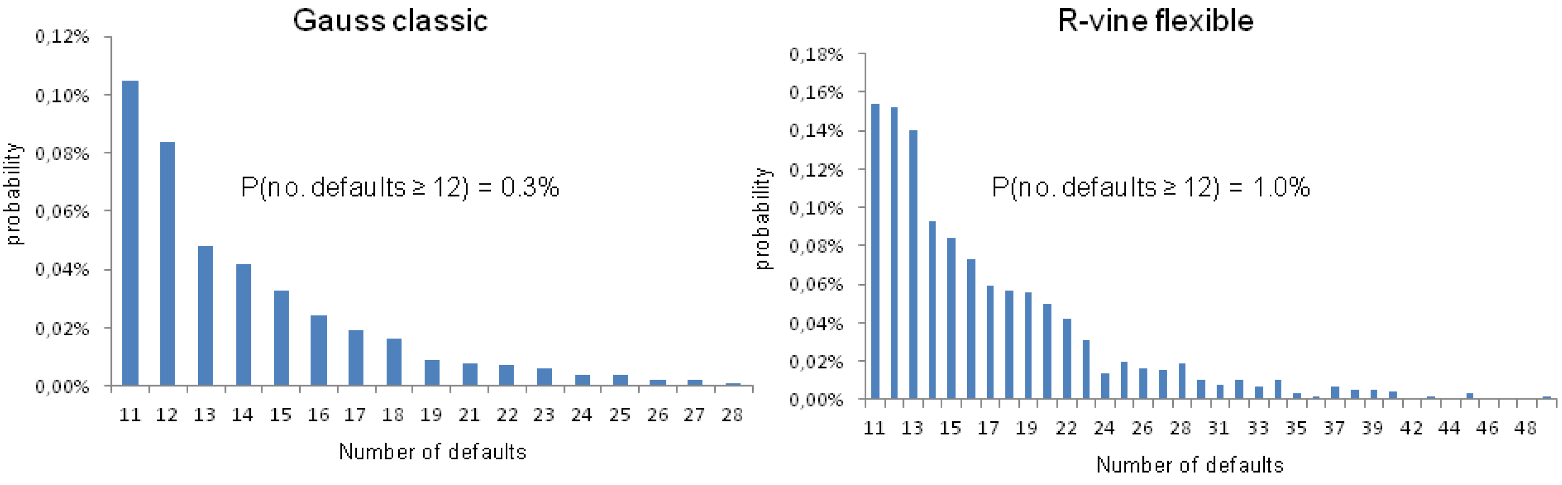
We define the tails of the loss distribution as ten defaults and more. Figure 6 shows the tails of the loss distribution for the reduced S&P 500 portfolio as predicted by a classic Gauss copula and by a flexible R-vine based on the training period up to March 2011. The chances of observing twelve or more defaults in our portfolio under the Gauss copula is 3:1000, while it is 1:100 under the flexible R-vine (below we will see why we are looking exactly at twelve defaults).

The interesting and essential backtesting question now is “How often did twelve or more defaults occur in the backtesting period”? Obviously, there were not many defaults of S&P 500 companies in the last 58 months, which is why looking at real-life defaults is of no help. However, note that we calibrated our model on a 1% default probability assumption and normal distributed equity returns, which allows us to evaluate how many companies have defaulted based on these model assumptions. In Section 3 the default threshold is given as $d_i={\Phi }^{-1}\left(P{D}_i\right)$. Applying $PD=1\%$ and calculating $d_i$ allows for counting how often the equity return of a company falls below $d_i$ in the backtesting period, which is the number of model-implied defaults. We justified the rather simplistic company-specific default assumptions because the correlation structure is the primary concern of this paper.

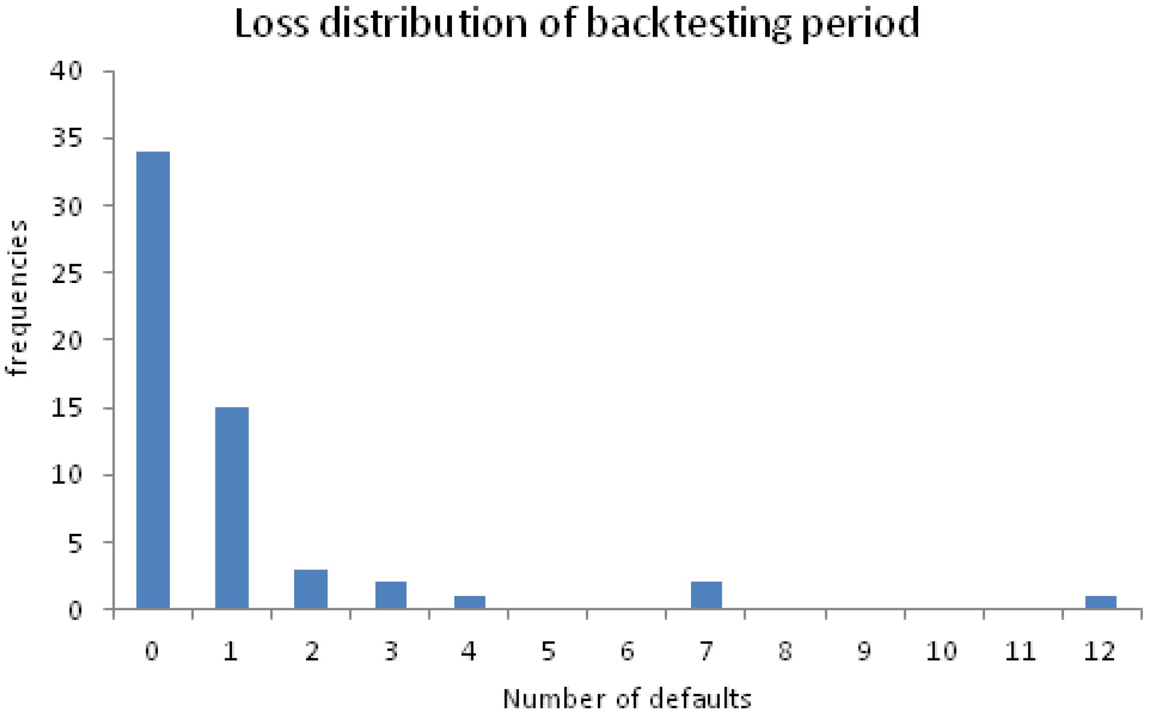
Figure 7 shows how many model-implied defaults occurred in the portfolio per month in the backtesting period (April 2011 to January 2016, 58 observations). For example, in 34 of the 58 backtesting months, no default occurred and the maximum number of defaults in a given month was twelve, which occurred once. Now, observing twelve defaults once in our backtesting period of 58 months is obviously closer to the prediction made by the flexible R-vine (1:100) than it is to Gauss copula prediction (3:1000). Our little backtesting analysis supports the well-known fact that the Gaussian copula is not suited to model portfolio tail events properly, while a flexible R-vine copula seems to do a way better job in this regard.

6. Conclusions

Especially in higher dimensions, Archimedean and elliptical copulas suffer from their inability to model asymmetric and complex dependence structures. The financial crisis of 2007–2008 established the need for an improved approach to model the correlation structure of credit portfolios. Vine copulas are an intuitive and convenient alternative to conventional copulas, which circumvent their shortcomings and which promise to be that improved approach. In this paper, we present how vine copulas can be used to derive a more accurate and more reliable estimate of the economic capital of a loan portfolio. We fit conventional and vine copulas separately to monthly equity returns from the Euro Stoxx 50 and S&P 500, and calculate the economic capital of the corresponding credit portfolios. We compare both copula approaches from a statistical and from an economic perspective.

Vine copulas enable us to model a more flexible and less restricted correlation structure compared to classical copulas, as replacing the latter by the former leads to an increased AIC. The better statistical fit to the data suggests that the modeled dependence structure is a more realistic model of the actual dependence structure and that, therefore, vine should be preferred to conventional copulas. When classic t and Clayton copulas are replaced by their corresponding D-vine structures, the economic capital is reduced. R-vine copulas in turn lead to a higher economic capital than D-vines. In the Gaussian case, conventional and vine copulas are equivalent. Mixing three bivariate copula families in a vine structure leads to the most accurate and reliable estimate for economic capital. Therefore, we provide statistically well-founded arguments that support the criticism of the role of the Gaussian copula in the financial crisis.

Despite its numerous and well-known shortcomings, the Gaussian copula is still the predominant tool in financial institutions when it comes to the modeling of the correlation structure of a credit portfolio. In this paper, we present a convenient and applicable alternative that should seriously be considered by risk managers in order to improve the methodology of credit portfolio risk modeling.