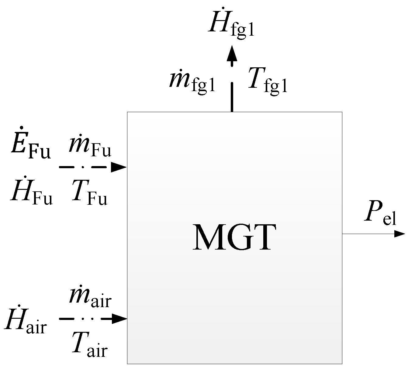
Article

Generic Combined Heat and Power (CHP) Model for the Concept Phase of Energy Planning Process

by
Satya Gopisetty
1,2,* and
Peter Treffinger
1
1
Department of Mechanical and Process Engineering, Offenburg University of Applied Sciences, Badstr. 24, 77652 Offenburg, Germany
2
Graduate School KleE, University of Freiburg, Georges-Koehler-Allee 106, 79110 Freiburg im Breisgau, Germany
*
Author to whom correspondence should be addressed.
Energies 2017, 10(1), 11; https://doi.org/10.3390/en10010011
Submission received: 7 November 2016 / Revised: 7 December 2016 / Accepted: 9 December 2016 / Published: 23 December 2016

Abstract

:
Micro gas turbines (MGTs) are regarded as combined heat and power (CHP) units which offer high fuel utilization and low emissions. They are applied in decentralized energy generation. To facilitate the planning process of energy systems, namely in the context of the increasing application of optimization techniques, there is a need for easy-to-parametrize component models with sufficient accuracy which allow a fast computation. In this paper, a model is proposed where the non-linear part load characteristics of the MGT are linearized by means of physical insight of the working principles of turbomachinery. Further, it is shown that the model can be parametrized by the data usually available in spec sheets. With this model a uniform description of MGTs from several manufacturers covering an electrical power range from 30 k W to 333 k W can be obtained. The MGT model was implemented by means of Modelica/Dymola. The resulting MGT system model, comprising further heat exchangers and hydraulic components, was validated using the experimental data of a 65 k W MGT from a trigeneration energy system.

1. Introduction

High fuel utilization factor, dual fuel capability, low emission levels and reliable self-generation are regarded as benefits of micro gas turbines (MGTs) as combined heat and power (CHP) units [1,2,3,4]. The first MGTs have been derived from jet engines. The most important application is in decentralized energy systems. The automotive application has not been successful so far. For decentralized energy systems, there is a trend towards polygeneration, i.e., the simultaneous generation of heat, electricity and cold from various energy sources which are often combined with district heating and/or district cooling systems. The increasing complexity of such systems is evident and a proper planning is a challenge. Simple but accurate models of the components are required in order to allow the investigation of concept variants with a reasonable effort. An important boundary condition is that only a few design parameters are initially fixed. That is why easy parametrization of the models is a must.
In this paper, a novel MGT system model for the energy planning process is proposed. The few parameters of the MGT model can be derived from the spec sheet data. The model gives the energy flows, fluid temperatures and mass flow rates which are essential with respect to the application in district heating and/or cooling networks. The MGT model was implemented by means of the open source object-oriented modeling language Modelica within the Dymola simulation environment [5]. Several different types of components such as prime movers, heat exchangers, storages, etc. can be combined and dimensioned to form a polygeneration system. The optimal energy scheduling of these components leads to an efficient operation at minimum energy costs for a given scenario [6]. For this reason and due to the linearization of the MGT model, it can be easily used for dimensioning or could also be applied in mathematical optimization methods or could be helpful when applying model-predictive control.

2. State-of-the-Art

A number of MGT models are reported in the literature due to the high importance of MGTs in decentralized energy systems [7]; their capability to be supplied with biomass [8]; the option to fire them externally [7,9]; and the option to combine them with a fuel cell leading to a high electrical efficiency [10,11]. Detailed models (white box models) are usually developed to support novel applications of MGTs, for example, the operation of MGT in combination with a biogas generator or a fuel cell. As these papers deal with in-depth design and/or control problems of specific machines, the respective models are very specific. For instance, they apply characteristic maps of particular compressors and turbines or polynomials are derived for a particular type of machine such as in [8,12,13,14]. This modeling approach is not suitable for system analysis in the concept phase of a project due to the high effort for parametrization. On the other hand, in many cases the requirements on the models for the concept phase of energy planning are only partly fulfilled. Several modeling approaches adopted in [8,12,13,15] are based on the detailed principles of turbomachinery and thermodynamics which tend to be too complicated for usage within the concept phase. Furthermore, some models are only partly validated like [16] or not validated as in [15,17], while others are either difficult to parametrize or the parametrization is not covered as in [13,18,19,20,21,22,23]. This situation might also be the reason why the authors in [7] recently stated that there is a lack of literature about the modeling, validation and parametrization of MGTs.
As already stated above, this paper contributes a novel model which can be applied in the concept phase of energy planning process of decentralized energy systems. Additionally, heat exchangers and hydraulic components which form the complete MGT system were also developed. They can also be parametrized with little information. The MGT system model was validated using experimental data from a real-time trigeneration energy system.

3. Energy Center: MGT System

Figure 1 shows the considered MGT system. It consists of the MGT itself and two heat exchangers in series to which the exhaust gas stream is supplied. The first heat exchanger, i.e., the exhaust gas heat exchanger of micro gas turbine (MGTHX) works above the dew point of the exhaust stream. The second heat exchanger, i.e., the condensing heat exchanger (CoHX) is designed for condensing conditions. The system includes hydraulic components, namely a valve and a couple of pumps on the supply side of heat exchangers. Both heat exchangers are supplied with water as heat transfer fluid. The MGT employs a regenerative Brayton cycle. Air is compressed by the air compressor and then preheated in the recuperator by means of hot exhaust gases. Natural gas is supplied to the combustion chamber. Finally, the mechanical power is generated by the expansion of exhaust gas in the turbine. Both the turbine and compressor are radial turbo-machines and are mounted together with the generator on a single shaft. This configuration is typical for MGTs. More detailed information to MGTs can be found in [4,24,25].
The MGT system shown in Figure 1 is a part of the Energy Center situated at Offenburg University of Applied Sciences. The Energy Center is a trigeneration system which supplies heating, cooling and electrical energy to the university campus. Further information about the Energy Center can be found in [26,27]. Table 1 lists the manufacturers and type designation of the MGT components. Additionally, Figure 1 includes the instrumentation of the MGT system. Temperatures and volume flow rates were measured. The electrical power output was also monitored. The measured data was used for the validation of models.

4. Modeling Strategy of the MGT System

4.1. MGT Model

As shown in Figure 2, an energy planner is interested in the input and output of the MGT, namely flow rates, temperatures and electrical power. An MGT model applied for planning purposes should be accurate under part load conditions. Additionally, it should cover the transient behavior. In the case of energy flow analysis, the time constant of the MGT can be neglected since it is very small compared to the time constants of other equipments such as boiler, storage, etc. However, the transient behavior of the MGT must be considered in the case of electrical power quality analysis which is not the scope of this work. Thus, the steady-state mass and energy balances are sufficient for the purpose of energy flow analysis. Equation (1) represents the overall mass balance of the MGT and Equation (2) describes the mass flow of air using the variable air ratio.
m ˙ Fu + m ˙ air m ˙ fg 1 = 0
where,
m ˙ air = λ × L min , Fu × m ˙ Fu
Equations (3)–(8) describe the overall energy balance, fuel power input, enthalpy of fuel stream, enthalpy of air stream, enthalpy of flue gas stream and gross mechanical power output, respectively. The gross mechanical power output includes the shaft work as well as the losses due to friction. The heat losses to the surroundings are neglected. The specific heat capacities at constant pressure are calculated using the fluid property data given in ([28], Part D3, pp. 301–417).
E ˙ Fu + H ˙ Fu + H ˙ air m ˙ fg 1 P mech , gross = 0
where,
E ˙ Fu = m ˙ Fu × H i , Fu
H ˙ Fu = m ˙ Fu × c p , Fu × ( T Fu T ref )
H ˙ air = m ˙ air × c p , air × ( T air T ref )
H ˙ fg 1 = m ˙ fg 1 × c p , fg 1 × ( T fg 1 T ref )
P mech , gross = P el η em , gross
Equation (9) corrects the electrical power output from the International Organization for Standardization (ISO) reference conditions (288.15 K , 101.325 k Pa , 60% relative humidity) due to the influence of altitude as well as the temperature of ambient air. A decrease in air density through an increase in altitude or temperature leads to a lower mass flow rate and results in a lower power output [29]. 
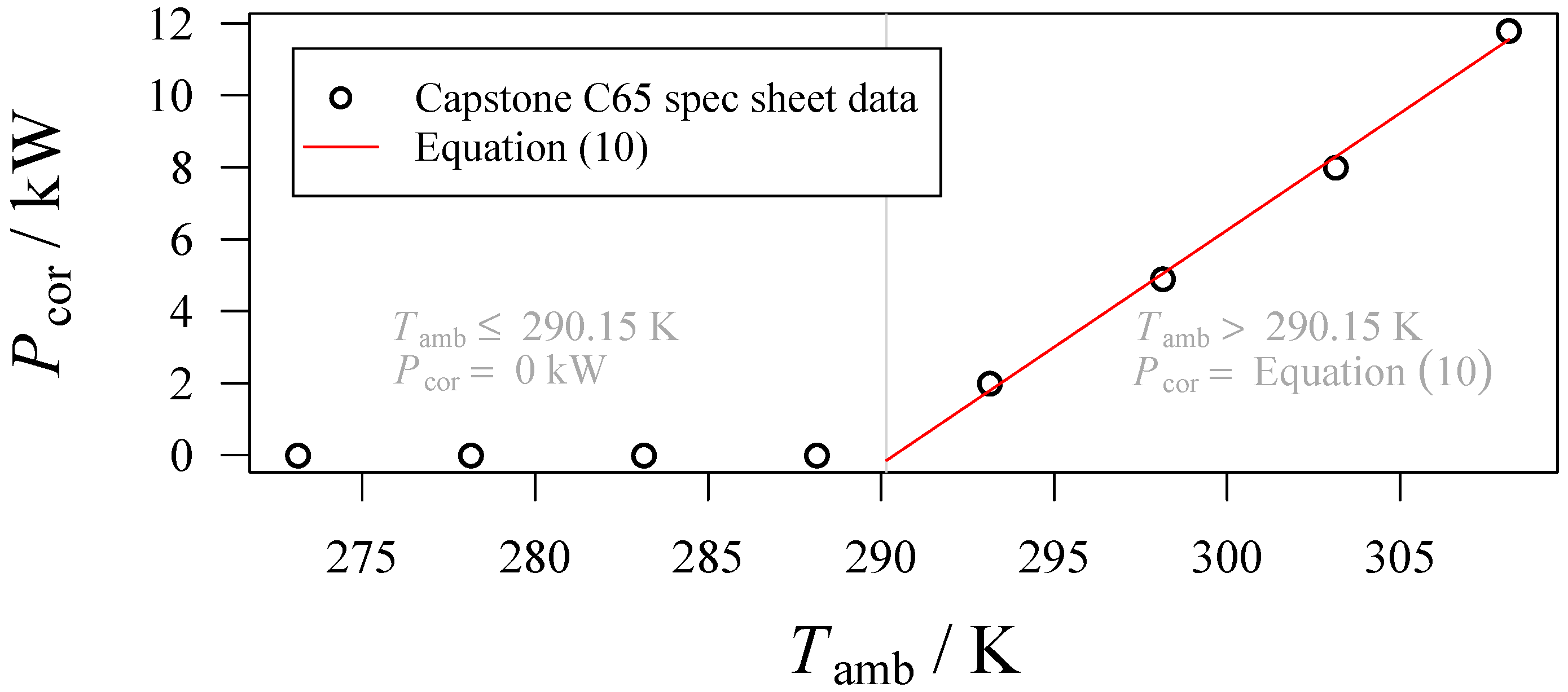
Figure 3 and Equation (10) depict the performance correction for Capstone C65 MGT based on the supplier test data ([30], Figure 3, p. 8 ). The coefficients a 0 and a 1 can be determined directly from the spec sheet data and their values are given in Table 2.
P el = P el , ISO P cor
where,
P cor = 0 if   T amb 290.15 a 0 + a 1 × T amb if   T amb > 290.15
Equation (11) shows the estimation of useful electrical power. In this case, the parasitic loads are the power consumed by power electronics system and fuel gas booster compressor.
P el , us = P el P par loads
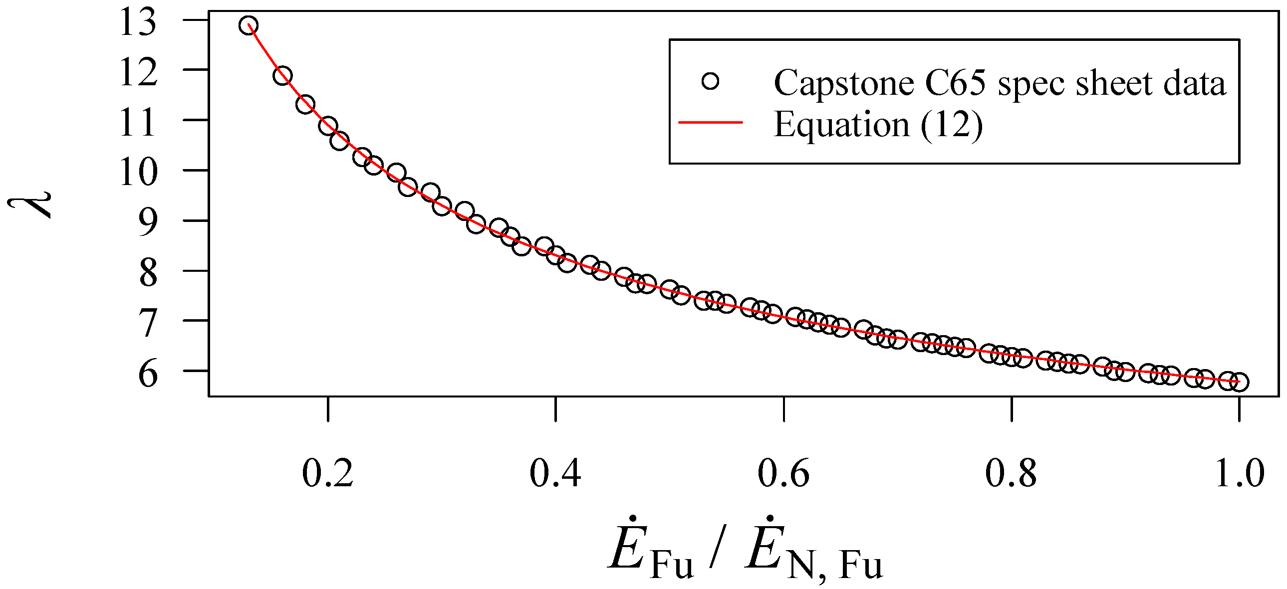
Figure 4 and Equation (12) illustrate the non-linear relationship between air ratio and fuel capacity percentage. Table 2 shows the coefficients b 0 and b 1 , and they can be derived directly from the spec sheet data using Equations (1) and (2).
λ = b 0 × E ˙ Fu E ˙ N , Fu b 1
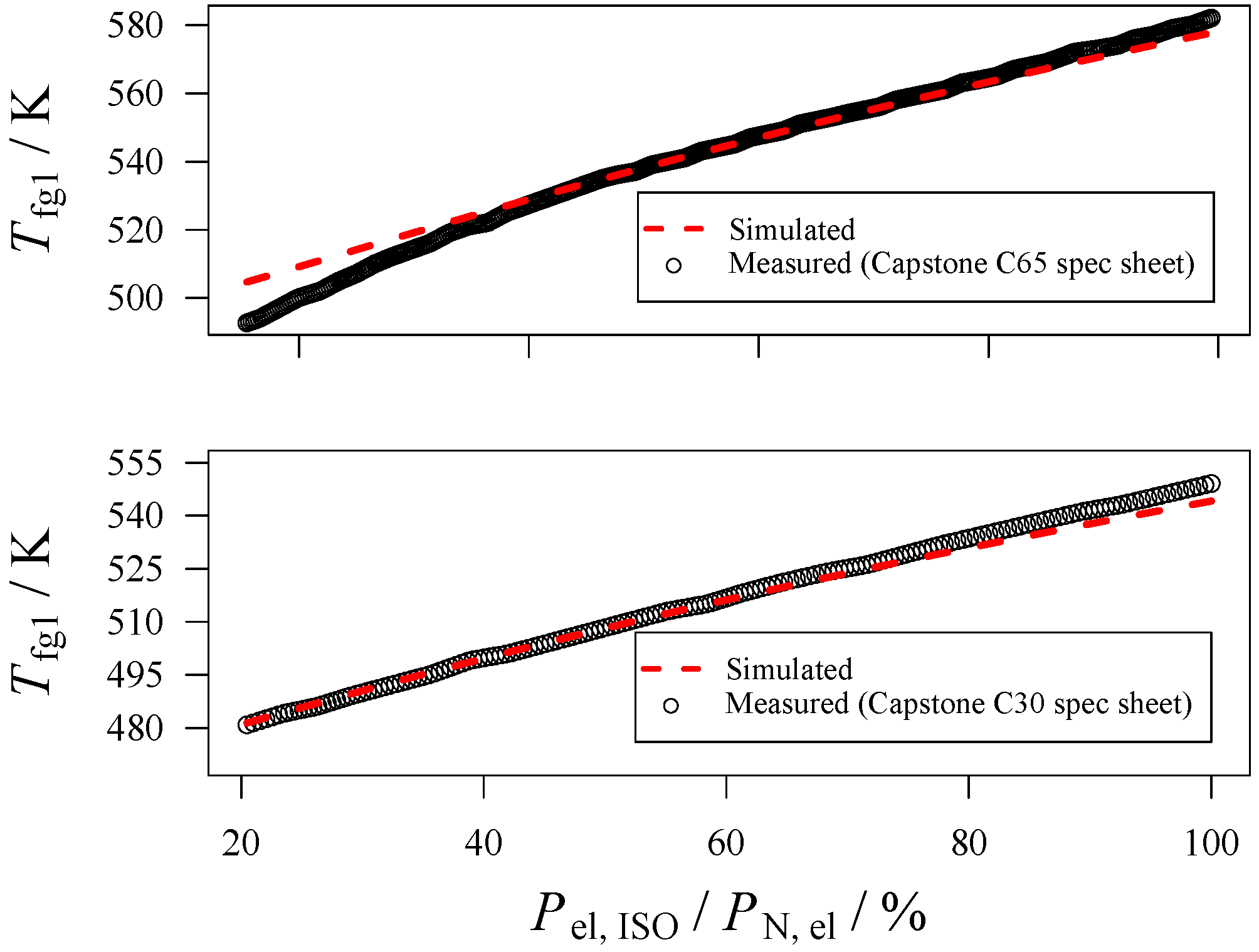
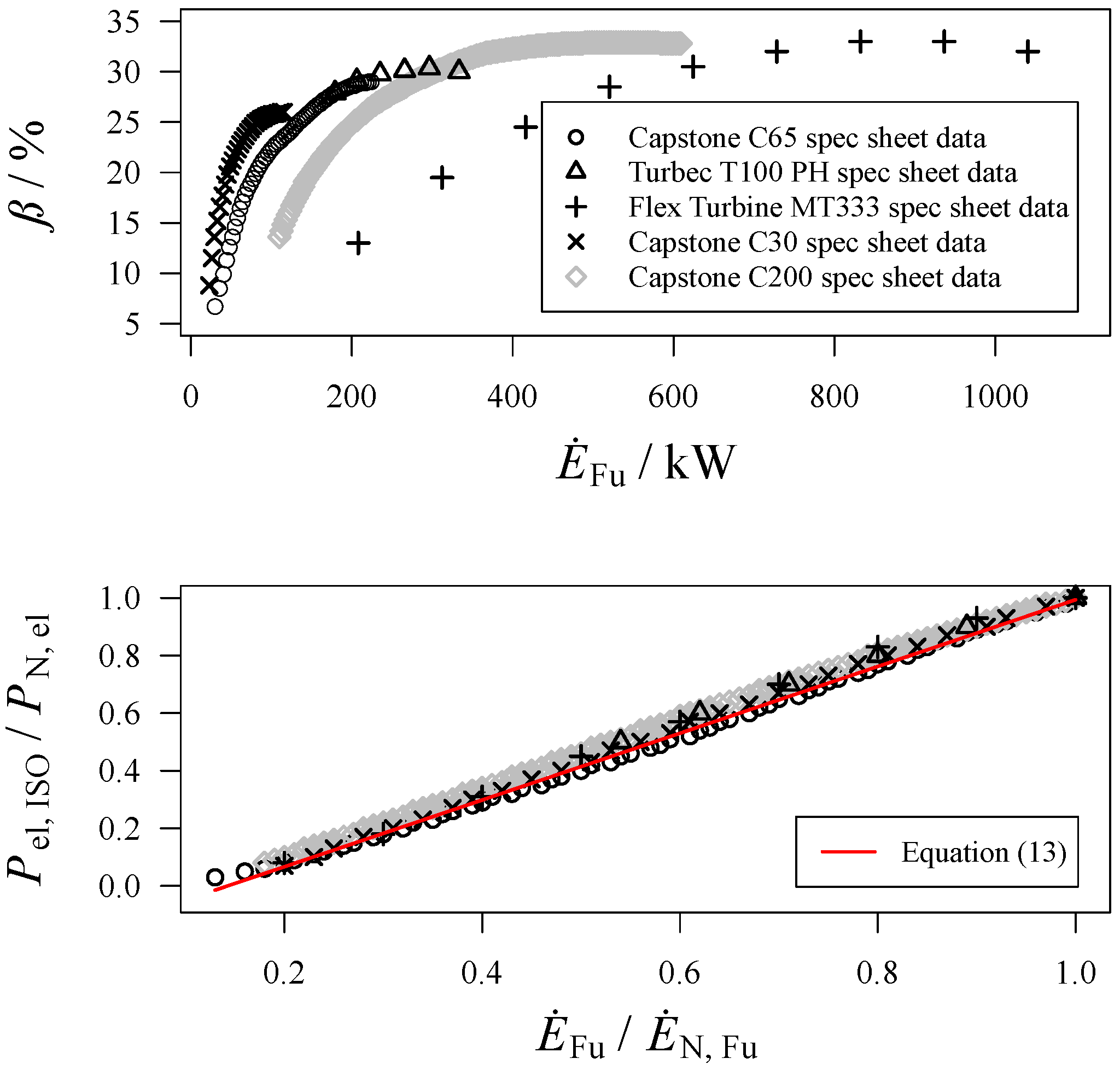
Figure 5 shows the non-linear part load behavior of electrical efficiency and fuel power for MGTs of different dimensions and manufacturers [30,31,32,33,34]. It is linearized by normalizing the electrical power and fuel power with their respective nominal values. The advantage of this approach is that any two points on the linearized curve can describe the complete part load behavior. The linearized lines can also be generalized to a linear curve fit with sufficient accuracy as shown in Figure 5 and Equation (13). This means that one full load and one part load point are enough to determine the coefficients c 0 and c 1 (see Table 2). Therefore, these coefficients are valid for the similar type of MGTs as in Figure 5. The behavior is linear because the mass flow of fuel is linearly proportional to the electrical power output. Moreover, all the linearized lines either overlap or are close enough to the curve fit with slightly varying slopes. This trend is due to the fixed turbine exit temperature, i.e., between 873.15 K and 923.15 K for the machines under consideration in Figure 5, and variable speed control to find the optimal operation line to achieve highest possible efficiency at full and part load. The optimal operation line is obtained by matching the compressor and turbine characteristic curves for a set of variables such as rotational speed, pressure ratio, inlet and outlet temperature, mass flow of air and fuel [24,35,36]. As most of the CHP machines operate either at full load or above 50% part load, the variation in the η em , gross , i.e., from the gross mechanical power output to the electrical power output, within this range is little owing to low frictional losses. Therefore, the η em , gross within this range is assumed to be a constant. It is tuned to 0.895 for the Capstone C65 machine through part load test using the spec sheet data.
P el , ISO P N , el = c 0 + c 1 × E ˙ Fu E ˙ N , Fu
The MGT developed using the above modeling approach consists of only four parameters (see Table 3) which can be found easily in the manufacturer’s spec sheet. Additionally, it consists of six fitting coefficients (see Table 2), namely a 0 and a 1 to describe the correction to electrical power output due to ambient conditions, b 0 and b 1 to describe the air ratio, and c 0 and c 1 to describe the part load behavior which can be generalized. As shown in Figure 3, Figure 4 and Figure 5, these coefficients can also be derived with a little effort using the spec sheet information.

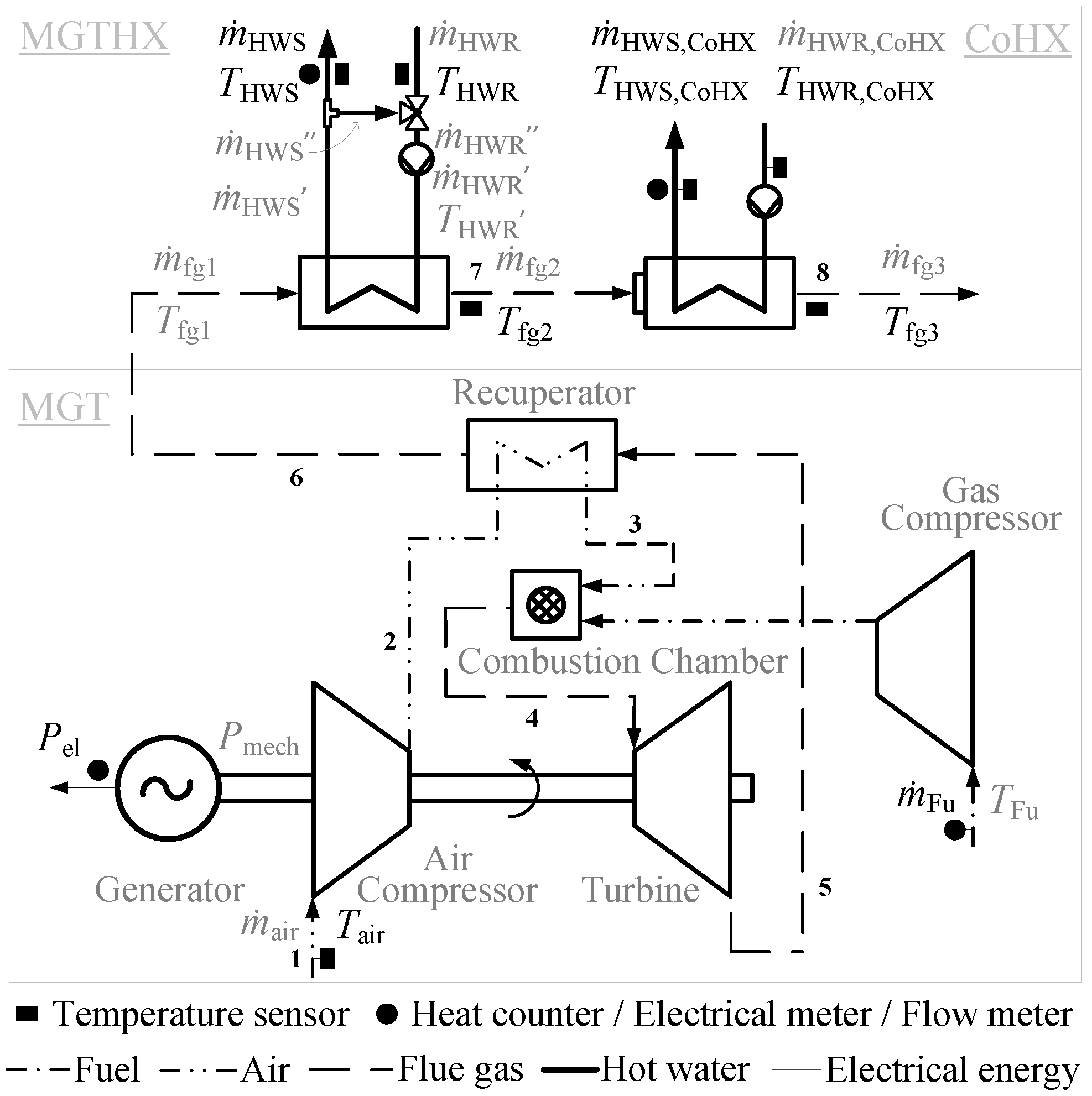
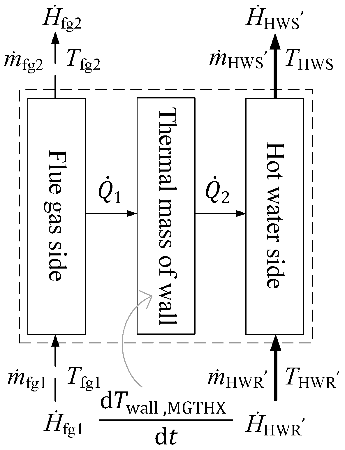
4.2. MGTHX and CoHX Model

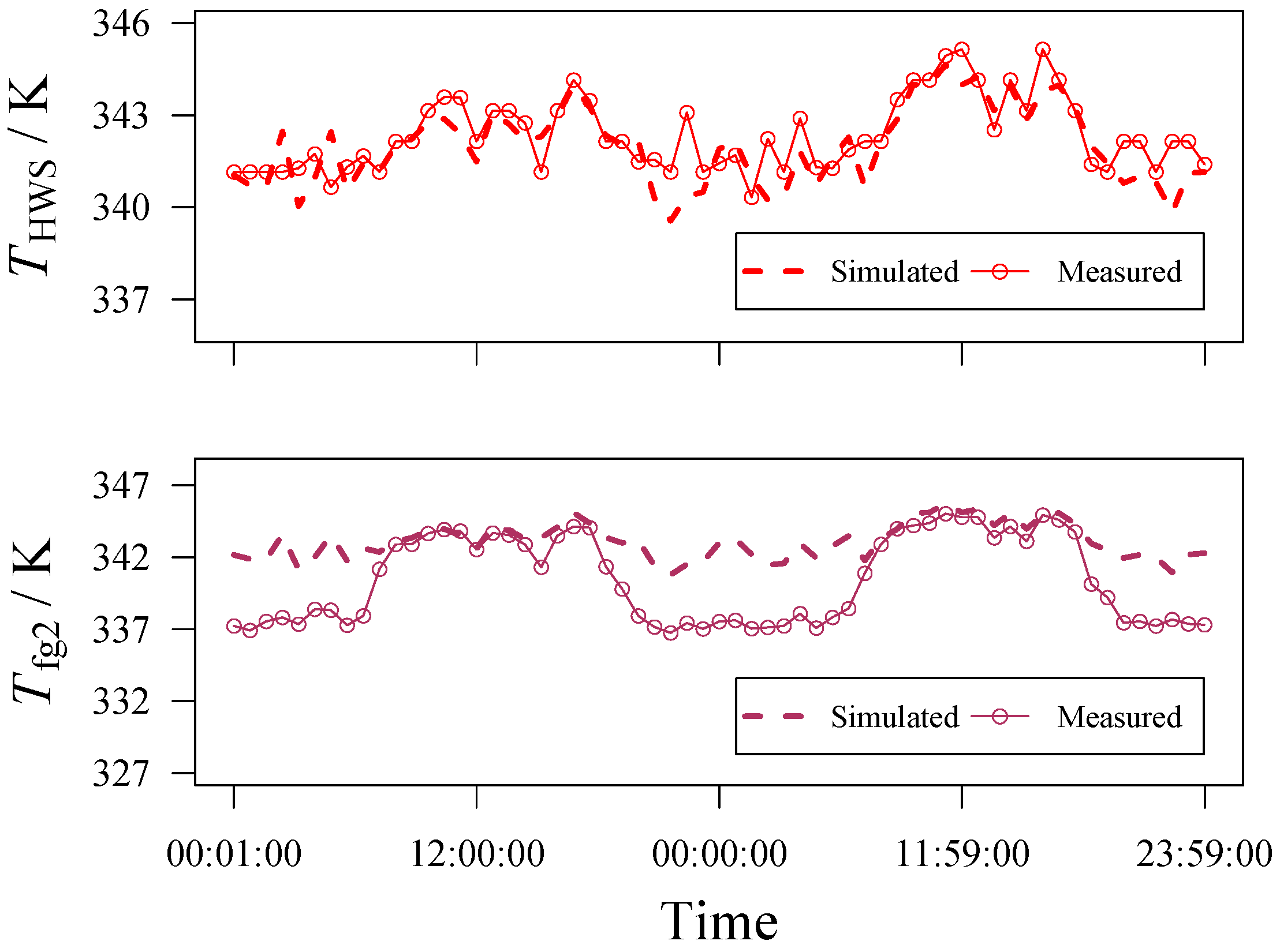
Figure 6 represents a simple but reasonable abstraction of the exhaust gas heat exchanger to describe the heat transfer from the flue gas side through the hot wall to the hot water side. Based on Newton’s law of cooling with constant wall temperature, Equations (14) and (15) can be derived to describe the inlet and outlet temperature of the flue gas pipe and the hot water pipe. A constant wall temperature is considered as the wall temperature is mainly determined by the hot water temperature.
( T fg , 2 T wall , MGTHX ) = ( T fg , 1 T wall , MGTHX ) × e G fg , MGTHX m ˙ fg 1 × c p , fg 1
( T HWS T wall , MGTHX ) = ( T HWR T wall , MGTHX ) × e G hw , MGTHX m ˙ HWR × c p , HWR
Equations (16)–(18) describe the energy balance on the flue gas side, hot water side and wall, respectively. The thermal capacities of flue gas and hot water are neglected as they are very small compared to that of the wall. Therefore, it is sufficient to describe the transients using the Equation (18).
H ˙ fg 1 H ˙ fg 2 Q ˙ 1 = 0
H ˙ HWR H ˙ HWS + Q ˙ 2 = 0
where,
Q ˙ 1 Q ˙ 2 = d E wall , MGTHX d t = C wall , MGTHX × d T wall , MGTHX d t
Table 4 shows the three parameters of MGTHX. The convective heat transfer coefficient on the flue gas side and the hot water side is estimated to be 250 W   m 2   K 1 and 909.1 W   m 2   K 1 , respectively. They are obtained by tuning the typical values given in ([28], Part B1, p. 20) to fit the simulation of outlet temperatures of MGTHX with the experimental measurements. The flue gas side heated surface area is considered to be the same as the hot water side heated surface area, i.e., 22 m 2 , given in the spec sheet [38]. Therefore, the product of convective heat transfer coefficient and heated surface area yields convective thermal conductance. The mass of wall is assumed to be half of the tare weight which is 308 k g , as given in the spec sheet [38]. The wall material is stainless steel 1.4571 for which the typical c p value is 500 J   k g 1   K 1 at 293.15 K [39]. The same value is considered for this case, as the change in c p value of stainless steel 1.4571 is little between 293.15 K and 493.15 K ([28], Part D6, p. 559). The thermal mass of wall is the product of the mass and specific heat capacity of wall. These parameters can be quickly estimated with a low effort.
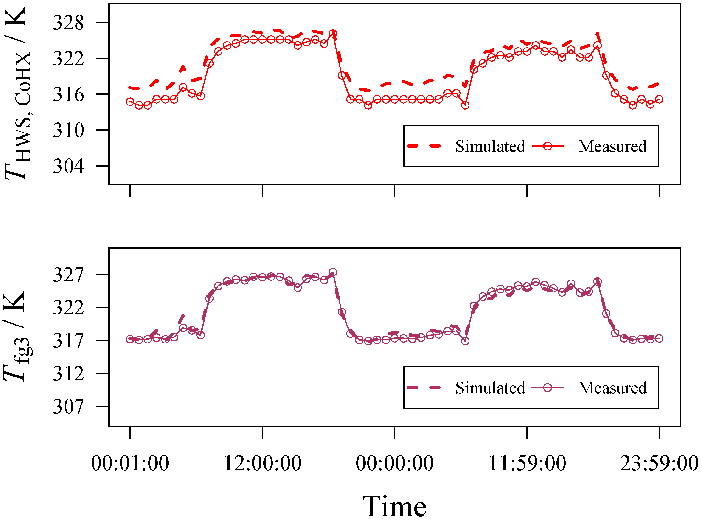
The CoHX model is similar to the above MGTHX model. Additionally, it consists of enthalpy of condensation in the energy balance equation on the flue gas side as shown in Equation (19). The dew point temperature of the water vapor present in the flue gases is estimated based on the mole fraction of carbon dioxide ([40], Figure 4, p. 5). The mass flow of condensate is calculated using Equation (20) where the parameter ϕ H 2 O is arbitrarily set to 37% based on the CoHX experiments at the Energy Center. In Equation (20), the mass fraction of water vapor in the flue gases is derived by means of the mole balance of combustion with the assumption that the natural gas is only composed of methane. Similar to the parametrization of the MGTHX model, the parameters of the CoHX model shown in Table 5 are determined using the spec sheet information and tuning the typical values of convective heat transfer coefficient. The mass of wall, c p value of stainless steel 1.4571, heated surface area, convective heat transfer coefficient on the flue gas side and the hot water side are 94 k g [41], 500 J   k g 1   K 1 [39], 11.33 m 2 [41], 250 W   m 2   K 1 and 500 W   m 2   K 1 ([28], Part B1, p. 20), respectively.
Q ˙ 3 = H ˙ fg 2 H ˙ fg 3 + m ˙ cond × Δ h c ( τ fg ) , if   T fg 3 τ fg H ˙ fg 2 H ˙ fg 3 , if   T fg 3 > τ fg
where,
m ˙ cond = ϕ H 2 O × w H 2 O , fg 2 × m ˙ fg 2

4.3. Hydraulic Components

Since the prime focus of this article is the modeling approach and parametrization of MGTs, only an overview of the hydraulic components of the MGT system is described. The pump model is developed using the affinity laws described in Equations (21) and (22) for constant impeller diameter. The reference values are for 100% nominal shaft speed.
h h ref = n shaft n ref , shaft 2
P shaft P ref , shaft = n shaft n ref , shaft 3
The characteristic curves of pump such as the dependence of head and electrical power on the fluid flow rate are illustrated in the manufacturer’s spec sheet [42]. Therefore, these characteristic curves are described as a function of third-order (Equation (23)) and fourth-order (Equation (24)) polynomial equation in the model. Equation (25) is used to estimate the reference shaft power.
h ref = f ( m ˙ hw )
P ref , el = f ( m ˙ hw )
P ref , shaft = P ref , el × η ref , motor
The advantage of this approach is that one characteristic curve is sufficient to describe the complete pump map. Therefore, a few or even three data points can describe the complete characteristic curve. An additional advantage is that the pump model consists of only one parameter, i.e., reference efficiency of pump’s motor, and nine fitting coefficients to describe the characteristic curves (Equations (23) and (24)). Similar to the pump model, the characteristics of the three-way valve model is described using the manufacturer’s spec sheet information [43]. The valve model consists of only one parameter, namely the flow coefficient at 100% valve opening and 1 bar pressure difference, and six fitting coefficients to describe the valve characteristics.
Another important component is the tee split where the pressure drop significantly determines the dimensions of its corresponding hydraulic components. In practice and also in literature, the kinetic energy term in tee split models is often neglected in the description of pressure drop which otherwise may hinder the foreseeing of reverse flow. This is a major reason why pressure drops are not accurately estimated. It should be noted that the correct estimation of pressure drops is essential during the project phase following the concept phase where the hydraulic engineering is more detailed. This term is included in this model to estimate pressure drops more accurately. Equation (26) defines the pressure drop in tee pipes ([44], p. 207). It consists of a kinetic energy term, a major frictional loss term due to pipe flow and a minor frictional loss term due to pipe fitting. The major friction loss term, i.e., the Darcy-Weisbach equation, is divided into two parts which consists of the velocity at inlet for the half of pipe length and the velocity at outlet for the other half to describe the average velocity through the run pipe. The pressure drop in the branch is also defined using a similar equation. Equations (27) and (28) show the kinetic energy factor ([44], Equation 4.135, p. 160) and its exponent ([44], Equation 4.133, p. 157) for the pipe inlet. A similar equation is used for the pipe and the branch outlet.
p HWS p HWS = α HWS × ρ HWS × u HWS 2 2 + α HWS × ρ HWS × u HWS 2 2 + f HWS × ( l pipe / 2 ) D pipe × ρ HWS × u HWS 2 2 + f HWS × ( l pipe / 2 ) D pipe × ρ HWS × u HWS 2 2 + ζ pipe × ρ HWS × u HWS 2 2
α HWS = ( s HWS + 1 ) × ( 2 s HWS + 1 ) 3 4 × 3 s HWS + 1 × 3 s HWS + 2 × s HWS 6
where,
s HWS 1 f HWS
The major friction loss in a pipe flow is described using the Darcy-Weisbach equation. The Haaland equation ([45], Equation (5), p. 89) is implemented at pipe inlet, branch and pipe outlet to estimate the Darcy friction factor as shown in Equation (29).
1 f HWS = 1.8 × log ϵ pipe / D pipe 3.7 1.11 + 6.9 R e HWS
The minor friction loss due to pipe fittings is described as the product of the kinetic head and the minor loss coefficient. The pipe and the branch minor loss coefficient for a 90 tee joint are taken from ([44], Figure 4.150a, p. 208). Therefore, the minor loss coefficients are expressed as a function of volume flow rate at branch outlet upon volume flow rate at pipe inlet in the tee model as shown in Equation (30).
ζ pipe ( or ) ζ branch = f V ˙ HWS V ˙ HWS
This approach leads to only six parameters for the tee split model, namely the length, diameter and roughness of the pipe as well as the branch. All the parameters of the hydraulic components described above are easily available either in the spec sheets or site layouts.

5. Results and Discussion

Figure 7 shows the part load verification of the black box MGT model using the spec sheet data for machines with different dimensions. MGTs operate mostly at a part load higher than 50% or at full load. The efficiency decreases drastically at part load less than 50% due to heat and frictional losses. Since the heat losses were neglected in the black box MGT model, it can be seen in Figure 7 that the discrepancy was high for part load less than 50%. This effect was more prominent in the machines with larger capacities.
Figure 8 shows the input signals of the MGT system model. The MGT at the Energy Center operates always at full load because it serves as a base load. The mass flow of fuel input was almost constant with slight disturbances due to the changes in intake pressure. The mass flow and return temperature of hot water changed according to the heat load demand. Figure 9 shows that the agreement between the measured data and the simulated data was at an acceptable level as the deviation between them was low with a maximum relative discrepancy of 5.5%. The useful electrical power trend similar (Figure 9) to the mass flow of the fuel input (Figure 8) because they are linearly proportional to each other as shown in Equation (13). The electrical power output at ISO conditions was corrected due to the influence of ambient air temperature as described in Section 4.1. The ambient air temperature fluctuated between 293 K and 294.5 K during the experimental time period. It can be seen in Figure 9 that there was a decrease in the electrical power output whenever there was an increase in the ambient air temperature.
Figure 10 and Figure 11 illustrate the transients of the hot water supply temperature and the flue gas temperature. MGTs have fast transients, for example, any changes in the mass flow of fuel, mass flow of hot water and hot water return temperature results in quick changes in the output temperatures due to the low thermal mass of these machines. These transients were described by the two states in this MGT system model, one each in the MGTHX and the CoHX model as shown in Equation (18). The initial values for these two states, namely T wall , MGTHX and T wall , CoHX , were set to 342.15 K and 317.15 K based on the experimental data of T HWS and T HWS , CoHX . The discrepancy between experimental and simulated results of T HWS and T HWS , CoHX was very low, i.e., a maximum relative discrepancy of 0.8% and 1.1% for T HWS and T HWS , CoHX on the Kelvin temperature scale for the experimental time period. The agreement between the measurement and the simulation of the flue gas temperature is comparatively better for the CoHX model than the MGTHX model. The maximum relative discrepancy for the MGTHX was 1.7% and that of the CoHX was 0.6% on the Kelvin temperature scale. The high deviation for the flue gas temperature of the MGTHX was due to the discrepancy of the valve opening signal which resulted in slightly higher mass flow of HWR and therefore higher T fg 2 .
Figure 12 shows the simulation of pressure drops in the tee split model. It can be seen in Figure 12 that pressure differences between the inlet and outlets were low. As already mentioned in the hydraulic components Section 4.3, the omission of the kinetic energy term in Equation (26) can lead to large pressure drops resulting in over-dimensioning of hydraulic components. It will therefore lead to suboptimal as well as unfavorable operation and control of a CHP plant.
A further feature of the MGT system model described above is that it can be used to estimate the CO 2 emission as shown in Figure 13. Since the natural gas being supplied at the Energy Center consists of 90.65 mol % methane [46], it was assumed that the fuel input is fully methane for the purpose of simplification. The CO 2 emission was estimated using the air ratio and the composition of products in methane combustion. It should be noted that the property data of incompressible fluids and ideal gases for these models were taken from ([28], Part D3, pp. 301–417). As per the spec sheet data of Capstone C65 [30], the mass flow of exhaust gases at full load operation is about 0.49 k g   s 1 [30]. Considering this value, it was verified that the discrepancy was low for the simulated mass flow of exhaust gases in Figure 13. It was about 2.3% for the experimental time period.

6. Conclusions

The outcomes are as follows:
  • The MGT model has only four parameters, namely nominal electrical power, nominal fuel power, gross electromechanical efficiency and parasitic loads power, which can be easily parametrized with a low effort using the spec sheet data, as described in the modeling strategy of MGT system Section 4. The validation results show that the deviation between the experimental data and the simulated data was low. For example, the maximum absolute discrepancy for the flue gas temperature at the exit of the MGT system was 1.8 K. A simple MGT model with four parameters and six fitting coefficients including experimental validation is not yet reported in the literature.
  • The novel modeling approach described in the MGT model Section 4.1 leads to the linearization of MGT’s non-linear part load characteristics. Therefore, the MGT machines can be easily dimensioned due to the linear characteristic between the normalized fuel input and the normalized electrical output (refer to Figure 5 in the MGT model Section 4.1). This approach is especially useful due to the little information available during the concept phase of energy planning.
  • The novel modeling approach can be generalized for similar type of MGT machines. The applicability was supported by the part load verification of two MGT machines with nominal capacities of 30 kW and 65 kW (Figure 7). The novel modeling approach was further supported by the experimental validation of an MGT machine with a nominal capacity of 65 kW (refer to the results and discussion Section 5). However, the approach could be confirmed if further experimental data are available for the MGT machines of different scales.
  • The computation time of the MGT system model was about 2.5 s for the simulation time interval of 47.97 h and output intervals of 2879. The default solver of Dymola, viz. DASSL, was used with a variable step size integration and a tolerance of 0.0001. The work station configuration was 64-bit Windows 7 operating system with Intel Core i7-2600 3.4 GHz and 8 GB RAM. Since the MGT model is computationally fast, it forms the basis for optimization.
  • Since Modelica/Dymola offers high flexibility [5] and also due to the generic nature of MGT model, the MGT model can be easily transferred to the next stages of energy planning or other applications. Therefore, it simplifies the energy planning process and help in making fast decisions and computations.
  • The MGT system model not only assists in dimensioning the MGT machine, but also in testing and dimensioning the hydraulic components to avoid reverse flows and understand pressure drops in the hydraulic circuits. It also helps in investigating the CO 2 emissions. These factors are very vital for a CHP design and operation.

Acknowledgments

This study is a part of the “KleE” project which was funded by the Baden-Württemberg Ministry of Science, Research and Arts (MWK). More information at https://www.klee.uni-freiburg.de/. The authors also thank Offenburg University of Applied Sciences for funding a part of this research work.

Author Contributions

The authors developed the concept. Satya Gopisetty performed the experiments, simulations and analyzed data. Peter Treffinger contributed with suggestions to physical modeling and implementation of models.

Conflicts of Interest

The authors declare no conflict of interest.

Abbreviations

The following abbreviations are used in this manuscript:
CHPCombined heat and power
CoHXCondensing heat exchanger
ISOInternational Organization for Standardization
MGTMicro gas turbine
MGTHXExhaust gas heat exchanger of micro gas turbine
VDIVerein Deutscher Ingenieure (in German)

Latin Letters

a , b , c Fitting coefficients
c p Specific heat capacity (J/(kg · K))
CThermal mass (J/K)
DDiameter (m)
E ˙ Energy flow (W)
fDarcy friction factor (-)
GThermal conductance (W/K)
gAcceleration due to gravity (m/ s 2 )
hHead (m)
Δ h c Specific enthalpy of condensation (kJ/kg)
HValve opening (%)
H i Lower heating value (kJ/kg)
H ˙ Enthalpy of stream (W)
k v s Flow coefficient of a fully open valve ( m 3 / h )
lLength (m)
L min Stoichiometric air-fuel ratio (-)
m ˙ Mass flow rate (kg/s)
nRotational speed (1/min)
PPower (W)
pPressure (Pa)
Q ˙ Heat flow (W)
R e Reynolds number (-)
R 2 Coefficient of determination (-)
SResidual standard error (-)
sKinetic energy factor exponent (-)
TTemperature (K)
uVelocity (m/s)
V ˙ Volumetric flow rate ( m 3 / s )
wMass fraction (-)

Greek Letters

α Kinetic energy factor (-)
βElectrical efficiency (%)
ηEfficiency (%)
ϵAbsolute roughness (mm)
λAir ratio (-)
ϕ H 2 O Percentage of water vapor condensed (%)
ρDensity (kg/ m 3 )
τDew point temperature (K)
ζMinor loss coefficient (-)

Subscripts

ambAmbient
condCondensate
corCorrection
elElectrical
emElectromechanical
FuFuel
fgFlue gas
hwHot water
HWRHot water return
HWSHot water supply
mechMechanical
NNominal
par-loadsParasitic loads
refReference
usUseful

References

  1. Jain, S.; Roy, S.; Aggarwal, A.; Gupta, D.; Kumar, V.; Kumar, N. Study on the Parameters Influencing Efficiency of Micro-gas Turbines—A Review. In Proceedings of the ASME 2015 Power Conference, San Diego, CA, USA, 28 June–2 July 2015; Paper No. POWER2015-49417. p. V001T09A006.
  2. Monteiro, E.; Moreira, N.A.; Ferreira, S. Planning of micro-combined heat and power systems in the Portuguese scenario. Appl. Energy 2009, 86, 290–298. [Google Scholar] [CrossRef]
  3. Pilavachi, P.A. Power generation with gas turbine systems and combined heat and power. Appl. Therm. Eng. 2000, 20, 1421–1429. [Google Scholar] [CrossRef]
  4. Pilavachi, P.A. Mini- and micro-gas turbines for combined heat and power. Appl. Therm. Eng. 2002, 22, 2003–2014. [Google Scholar] [CrossRef]
  5. Fritzson, P.; Bunus, P. Modelica–A General Object-Oriented Language for Continuous and Discrete-Event System Modeling and Simulation. In Proceedings of the 35th Annual Simulation Symposium, San Diego, CA, USA, 14–18 April 2002; pp. 365–380.
  6. Moradi, H.; Abtahi, A.; Esfahanian, M. Optimal energy management of a smart residential combined heat, cooling and power. Int. J. Tech. Phys. Probl. Eng. 2016, 8, 9–16. [Google Scholar]
  7. Rahman, M.; Malmquist, A. Modeling and simulation of an externally fired micro-Gas turbine for standalone polygeneration application. J. Eng. Gas Turbines Power 2016, 138, 112301. [Google Scholar] [CrossRef]
  8. Riccio, G.; Chiaramonti, D. Design and simulation of a small polygeneration plant cofiring biomass and natural gas in a dual combustion micro gas turbine (BIO_MGT). Biomass Bioenergy 2009, 33, 1520–1531. [Google Scholar] [CrossRef]
  9. Camporeale, S.M.; Ciliberti, P.D.; Fortunato, B.; Torresi, M.; Pantaleo, A.M. Externally Fired Micro Gas Turbine and ORC Bottoming Cycle: Optimal Biomass/Natural Gas CHP Configuration for Residential Energy Demand. In Proceedings of the ASME Turbo Expo 2015: Turbine Technical Conference and Exposition, Montréal, QC, Canada, 15–19 June 2015; Paper No. GT2015-43571. p. V003T06A020.
  10. Ferrari, M.L.; Liese, E.; Tucker, D.; Lawson, L.; Traverso, A.; Massardo, A.F. Transient modeling of the NETL hybrid fuel cell/gas turbine facility and experimental validation. J. Eng. Gas Turbines Power 2007, 129, 1012–1019. [Google Scholar] [CrossRef]
  11. Ghigliazza, F.; Traverso, A.; Pascenti, M.; Massardo, A.F. Micro Gas Turbine Real-Time Modeling: Test Rig Verification. In Proceedings of the ASME Turbo Expo 2009: Power for Land, Sea and Air, Orlando, FL, USA, 8–12 June 2009; Paper No. GT2009-59124. Volume 5, pp. 29–36.
  12. Camporeale, S.M.; Fortunato, B.; Torresi, M.; Turi, F.; Pantaleo, A.M.; Pellerano, A. Part Load Performance and Operating Strategies of a Natural Gas-Biomass Dual Fuelled Microturbine for CHP Generation. In Proceedings of the ASME Turbo Expo 2014: Turbine Technical Conference and Exposition, Düsseldorf, Germany, 16–20 June 2014; Paper No. GT2014-27109. p. V03AT07A033.
  13. Aklilu, B.T.; Gilani, S.I. Mathematical modeling and simulation of a cogeneration plant. Appl. Therm. Eng. 2010, 30, 2545–2554. [Google Scholar] [CrossRef]
  14. Kolka, Z.; Kalous, J.; Biolkova, V.; Biolek, D. Simulation Model of Microturbine Unit. In Proceedings of the 15th International Conference on Intelligent Engineering Systems, Poprad, Slovakia, 23–25 June 2011; pp. 431–434.
  15. Malinowski, L.; Lewandowska, M. Analytical model-based energy and exergy analysis of a gas microturbine at part-load operation. Appl. Therm. Eng. 2013, 57, 125–132. [Google Scholar] [CrossRef]
  16. Basrawi, F.; Yamada, T.; Nakanishi, K.; Naing, S. Effect of ambient temperature on the performance of micro gas turbine with cogeneration system in cold region. Appl. Therm. Eng. 2011, 31, 1058–1067. [Google Scholar] [CrossRef]
  17. Basrawi, M.F.B.; Yamada, T.; Nakanishi, K.; Katsumata, H. Analysis of the performances of biogas-fuelled micro gas turbine cogeneration systems (MGT-CGSs) in middle- and small-scale sewage treatment plants: Comparison of performances and optimization of MGTs with various electrical power outputs. Energy 2012, 38, 291–304. [Google Scholar] [CrossRef]
  18. Saha, A.K.; Chowdhury, S.; Chowdhury, S.P.; Crossley, P.A. Modeling and performance analysis of a microturbine as a distributed energy resource. IEEE Trans. Energy Convers. 2009, 24, 529–538. [Google Scholar] [CrossRef]
  19. Chan, Y.K.; Gu, J.C. Modeling and Simulation of Microturbine and Renewable Energy Resources for Distributed Generation System. In Proceedings of the 8th Asian Control Conference, Kaohsiung, Taiwan, 15–18 May 2011; pp. 590–595.
  20. Zhu, Y.; Tomsovic, K. Development of models for analyzing the load-following performance of microturbines and fuel cells. Electr. Power Syst. Res. 2002, 62, 1–11. [Google Scholar] [CrossRef]
  21. Haugwitz, S. Modelling of microturbine systems. In Proceedings of the European Control Conference (ECC) 2003, Cambridge, UK, 1–4 September 2003; pp. 1234–1239.
  22. Naing, S.; Yamada, T.; Nakanishi, K. Renewable fuel utilization in a cogeneration arrangement with hydrate storage method. J. Power Energy Syst. 2007, 1, 239–250. [Google Scholar] [CrossRef]
  23. Školník, P.; Hubka, L.; Modrlák, O.; Náhlovský, T. Cogeneration Units Simulation Models Library. In Proceedings of the 19th International Conference on Process Control, Štrbské Pleso, Slovakia, 18–21 June 2013; pp. 252–256.
  24. Kim, T.S.; Hwang, S.H. Part load performance analysis of recuperated gas turbines considering engine configuration and operation strategy. Energy 2006, 31, 260–277. [Google Scholar] [CrossRef]
  25. Lee, J.J.; Yoon, J.E.; Kim, T.S.; Sohn, J.L. Performance test and component characteristics evaluation of a micro gas turbine. J. Mech. Sci. Technol. 2007, 21, 141–152. [Google Scholar] [CrossRef]
  26. Gopisetty, S.; Treffinger, P. Energy Analysis of Trigeneration based on Scarce Data. In Proceedings of the 10th International Conference on the European Energy Market (EEM), Stockholm, Sweden, 27–31 May 2013; pp. 1–7.
  27. Gopisetty, S.; Treffinger, P. Innovative combined cooling, heat and power (Trigeneration) at Offenburg University of Applied Sciences. Environ. Biotechnol. 2013, 9, 25–37. [Google Scholar]
  28. VDI Heat Atlas, 2nd ed.; Springer: Berlin/Heidelberg, Germany, 2010.
  29. Meher-Homji, C.B.; Chaker, M.A.; Motiwala, H.M. Gas turbine performance deterioration. In Proceedings of the 30th Turbomachinery Symposium, Houston, TX, USA, 17–20 September 2001; pp. 139–175.
  30. Capstone Model C65 Performance; Technical Reference; Capstone Turbine Corporation: Chatsworth, CA, USA, 2008.
  31. T100 Microturbine System; Technical Description; Turbec S.p.A.: Corporeno, Italy, 2009.
  32. Flex Turbine MT333; Technical Specification; FlexEnergy Inc.: Portsmouth, NH, USA, 2013.
  33. Capstone Model C30 Performance; Technical Reference; Capstone Turbine Corporation: Chatsworth, CA, USA, 2006.
  34. Capstone C200 Microturbine; Technical Reference; Capstone Turbine Corporation: Chatsworth, CA, USA, 2009.
  35. Wang, W.; Cai, R.; Zhang, N. General characteristics of single shaft microturbine set at variable speed operation and its optimization. Appl. Therm. Eng. 2004, 24, 1851–1863. [Google Scholar] [CrossRef]
  36. Backman, J.L.H.; Kaikko, J. Microturbine systems for small combined heat and power (CHP) applications. In Small and Micro Combined Heat and Power (CHP) Systems: Advanced Design, Performance, Materials and Applications; Beith, R., Ed.; Woodhead Publishing Series in Energy; Woodhead Publishing Limited: Cambridge, UK, 2011; pp. 147–178. [Google Scholar]
  37. Energy Systems—Combined Heat and Power—Terms, Definitions, Examples; VDI 4608 Part 1 Guideline; Association of German Engineers (VDI): Düsseldorf, Germany, 2005.
  38. Rauchgaskühler 390A/TE RVS 122 kW; Spezifikationsblatt; Enalco, B.V.: Maasdijk, The Netherlands, 2006. (In German)
  39. Edelstahl X6CrNiMoTi17-12-2 1.4571; Werkstoffdatenblatt; Deutsche Edelstahlwerke GmbH: Witten, Germany, 2015. (In German)
  40. Brennwerttechnik für Wirtschaftlichkeit und Umweltschonung; Fachreihe Brennwerttechnik; Viessmann Werke GmbH & Co. KG: Allendorf (Eder), Germany, 2006. (In German)
  41. Rauchgaskühler 390A/TE RVS 17 kW; Spezifikationsblatt; Enalco (Holland) B.V.: Maasdijk, The Netherlands, 2006. (In German)
  42. MAGNA 32-120 F; Datenblatt; Grundfos GmbH: Erkrath, Germany, 2011. (In German)
  43. Dreiwegventile PN16 mit Flanschanschluss VXF40; Datenblatt; Siemens Schweiz AG: Zürich, Switzerland, 2013. (In German)
  44. Bohl, W.; Elmendorf, W. Inkompressible Strömungen. In Technische Strömungslehre, 14th ed.; Vogel Industrie Medien GmbH & Co. KG: Würzburg, Germany, 2008; pp. 83–304. (In German) [Google Scholar]
  45. Haaland, S.E. Simple and explicit formulas for the friction factor in turbulent pipe flow. J. Fluids Eng. 1983, 105, 89–90. [Google Scholar] [CrossRef]
  46. Erdgas Kenngrößen und Erdgas-Analyse; Datenblatt; badenovaNETZ GmbH: Freiburg, Germany, 2012. (In German)
Figure 1. Instrumentation type and measurement points position of the MGT system at the Energy Center. The measured signals are highlighted in black font color.
Energies 10 00011 g001
Figure 2. Black box MGT model which is an abstraction of the MGT shown in Figure 1.
Energies 10 00011 g002
Figure 3. Power correction vs. ambient air temperature at an altitude of 157 m for Capstone C65 MGT. The R 2 of the linear fit is 0.99.
Energies 10 00011 g003
Figure 4. Air ratio vs. fuel capacity percentage of Capstone C65 MGT at ISO conditions. The S of the curve fit is 0.049 on 62 degrees of freedom.
Energies 10 00011 g004
Figure 5. (Top) Electrical efficiency (According to the guideline VDI 4608 Part 1 ([37], pp. 18–19), the symbols α and β refer to the thermal and electrical efficiency in order to differentiate the energy quality grade of electricity and heat of a CHP unit.) vs. fuel power of different machines describing the part load behavior at ISO conditions; (Bottom) Normalized electrical power vs. normalized fuel power describing the part load behavior at ISO conditions. Equation (13) describes the linear curve fit for Capstone C65 machine. The R 2 value of the linear curve fit is about 0.98.
Energies 10 00011 g005
Figure 6. Grey box abstraction of the MGTHX. It consists of a flue gas and hot water pass separated by a wall.
Energies 10 00011 g006
Figure 7. (Top) Flue gas temperature at the outlet of the MGT vs. electrical load of the Capstone C65 MGT with a nominal electrical power of 65 kW ; (Bottom) Flue gas temperature at the outlet of the MGT vs. electrical load of the Capstone C30 MGT with a nominal electrical power of 30 kW . In both the cases, the relative discrepancy on the Kelvin temperature scale was less than 1% for a part load operation higher than 50%.
Energies 10 00011 g007
Figure 8. Input signals for the validation of the MGT system model, namely mass flow rates, temperatures and valve opening over time. The one minute time interval signals of the Capstone C65 MGT were for the experimental time period from 20 to 21 November 2013. Note: The pumps in the MGTHX and CoHX hot water circuit operated at a constant speed of 60% and 50%, respectively, during the experiment. The input pressure signal was set to 1.1 bar for the MGTHX and CoHX hot water circuit.
Energies 10 00011 g008
Figure 9. Useful electrical power of the MGT and ambient air temperature vs. time. The simulated values were obtained by means of the input signals specified in Figure 8. The maximum absolute discrepancy for P el , us was about 3 kW.
Energies 10 00011 g009
Figure 10. (Top) Hot water supply temperature at the outlet of the MGTHX’s hydraulic loop over time; (Bottom) Flue gas temperature at the outlet of the MGTHX over time. The simulated data was obtained by means of the input signals given in Figure 8. The maximum absolute discrepancy for T HWS and T fg 2 was about 2.7 K and 5.7 K .
Energies 10 00011 g010
Figure 11. (Top) Hot water supply temperature of the CoHX vs. time; (Bottom) Flue gas temperature at the outlet of the CoHX vs. time. The simulated data was obtained by means of the input signals specified in Figure 8. The maximum absolute discrepancy for T HWS , CoHX and T fg 3 was about 3.4 K and 1.8 K .
Energies 10 00011 g011
Figure 12. Inlet and outlet pressures of the tee split vs. time. The simulated values were obtained by means of the input signals specified in Figure 8.
Energies 10 00011 g012
Figure 13. (Top) Mass flow of exhaust gases vs. time; (Bottom) Mass fraction of CO 2 vs. time. The simulated values were obtained by means of the input signals specified in Figure 8.
Energies 10 00011 g013
Table 1. Nameplate information of the MGT system.
ComponentManufacturer and TypeCapacity
MGTCapstone C65 P N = 65 kW
MGTHXVerdesis/Enalco 390A-TE RVS Q ˙ N = 127 kW
CoHXVerdesis/Enalco 390A-TE RVS Q ˙ N = 16.8 kW
PumpsGrundfos 32-120 FMaximum h = 12 m
ValveSiemens VXF40.40 k v s = 19 m 3   h 1
Table 2. List of empirical coefficients describing the Capstone C65 MGT black box model.
Symbol a 0 a 1 b 0 b 1 c 0 c 1
Value−188.750.655.784−0.394−0.1651.159
Table 3. Parameters of the MGT black box model.
ParameterDescriptionValueUnit
P N , el Nominal electrical power65kW
E ˙ N , Fu Nominal fuel power224kW
η em , gross Gross electromechanical efficiency89.5%
P par loads Power electronics and fuel gas booster power7.5kW
Table 4. Parameters of the MGTHX grey box model.
ParameterDescriptionValueUnit
G fg , MGTHX Thermal conductance on the flue gas side5500W/K
G hw , MGTHX Thermal conductance on the hot water side20000W/K
C wall , MGTHX Thermal mass of wall77000J/K
Table 5. Parameters of the CoHX grey box model.
ParameterDescriptionValueUnit
G fg , CoHX Thermal conductance on the flue gas side2832.5W/K
G hw , CoHX Thermal conductance on the hot water side5665W/K
C wall , CoHX Thermal mass of wall47000J/K
ϕ H 2 O Percentage of water vapor condensed37%

