A Lyapunov Stability Theory-Based Control Strategy for Three-Level Shunt Active Power Filter

Abstract

The three-phase three-wire neutral-point-clamped shunt active power filter (NPC-SAPF), which most adopts classical closed-loop feedback control methods such as proportional-integral (PI), proportional-resonant (PR) and repetitive control, can only output 1st–25th harmonic currents with 10–20 kHz switching frequency. The reason for this is that the controller design must make a compromise between system stability and harmonic current compensation ability under the condition of less than 20 kHz switching frequency. To broaden the bandwidth of the compensation current, a Lyapunov stability theory-based control strategy is presented in this paper for NPC-SAPF. The proposed control law is obtained by constructing the switching function on the basis of the mathematical model and the Lyapunov candidate function, which can avoid introducing closed-loop feedback control and keep the system globally asymptotically stable. By means of the proposed method, the NPC-SAPF has compensation ability for the 1st–50th harmonic currents, the total harmonic distortion (THD) and each harmonic content of grid currents satisfy the requirements of IEEE Standard 519-2014. In order to verify the superiority of the proposed control strategy, stability conditions of the proposed strategy and the representative PR controllers are compared. The simulation results in MATLAB/Simulink (MathWorks, Natick, MA, USA) and the experimental results obtained on a 6.6 kVA NPC-SAPF laboratory prototype validate the proposed control strategy.

1. Introduction

The increased application of power electronics (variable frequency drives, AC-DC converters, etc.) causes serious harmonic pollution in power systems [1,2]. The active power filter (APF) is considered an effective solution for harmonic elimination of nonlinear loads [3,4,5,6,7,8,9,10,11,12,13,14,15].

The classical closed-loop feedback control scheme of the shunt active power filter (SAPF) includes indirect [3,4,5,6,7,8,9] and direct current control methods [10,11,12,13,14]. Proportional-resonant (PR) controllers are the most popular method for SAPF, as they guarantee zero-state errors and achieve the required total harmonic distortion (THD) performance at each specified frequency. The systematical design method of PR controllers is described in [3] and the effects of different discretization methods are considered, but the output harmonic order is below the 20th. An LCL-filter-based SAPF with PR controllers is proposed in [4], and the grid current spectrum shows that it has good compensation performance below the 25th harmonics but poor performance on eliminating switching frequency harmonics. A sensorless control strategy with multiple quasi-resonant compensators for SAPF was presented in [5], which is able to track an unknown grid frequency, reducing its sensitivity to this variable. However, the SAPF only outputs the 1st–15th harmonics and the THD of grid currents is up to 9.8%. In [6], a fixed-point processor-based PR current control scheme in synchronous reference frame (SRF) is proposed. It has a better response time compared with other frequency-selective current control methods, but it only outputs 1st–19th harmonics. Repetitive controllers just designed below 1.25 kHz are described in [7,8,9]. An improved repetitive controller which adds a proportional link in parallel with the original repetitive control loop for SAPF is proposed in [7]. The SAPF obtains good performance in simulation results, but only compensates to the 25th harmonics under experimental conditions. A two-layer structure controller is designed in [8]. The outer layer uses a repetitive control algorithm to provide good tracking of periodic signals and the inner layer achieves practically-decoupled control of d-axis and q-axis currents, while the compensation current order only reaches to 19th harmonic. A current control strategy integrating PR and odd-harmonic repetitive control (OHRC) is proposed in [9]. The OHRC method provides better performance than the multiple resonant control scheme, however these two methods only consider 1st–13th harmonics. SAPFs adopted hysteresis controllers are presented in [10,11,12], which only output 1st–21st harmonics, moreover the output currents are magnified between the 21st–33rd harmonics in [11,12].

The aforementioned SAPFs with closed-loop control methods only have good compensation performance below the 25th harmonics. The reason for this is that the output bandwidth is determined jointly by the control parameters, output inductance and switching frequency. The general switching frequency of insulated gate bipolar transistors (IGBT) is 10–20 kHz. Under the specified switching frequency, the output bandwidth is determined by the proportional gain of the controller and output inductance. From their open-loop Bode plots, it can be concluded that a larger proportional gain and smaller inductance means a wider output bandwidth, however this situation leads to worse current ripple inhibition ability [16]. This compromise between system stability and harmonic current compensation ability indicates that they cannot deal with the high-frequency harmonics. However, in the metal processing industry, the Intermediate Frequency Induction Heating Device (IFIHD) typically generate about 1st–49th harmonics. The high-frequency harmonics cannot satisfy the requirements of IEEE Standard 519-2014 [17], which may cause interference with communication circuits and increase total losses of transformers.

Lyapunov stability theory was introduced in inverters [18,19,20,21,22,23,24], since it can ensure the globally asymptotical stability of nonlinear systems. Lyapunov stability theory-based method uses the reference currents and system mathematical model to obtain gate signals, which overcomes the disadvantage of the classical closed-loop feedback control method. As a result, Lyapunov stability theory is suitable for improving the compensation ability on the premise of system stability.

In a neutral-point-clamped shunt active power filter (NPC-SAPF) system, the upper and lower DC-capacitor voltages have to be maintained at half of the DC-link voltage, because the balance of upper and lower DC-capacitor voltages is related to the system stability and compensation performance. The carrier based pulse width modulation (CB-PWM) in [25,26,27] achieves the voltage-balancing task and mitigates the voltage oscillations of neutral-point (NP) with lower switching losses than other PWM methods. Moreover, it is easy to realize and saves more storage space in digital implementation than the NP voltage balance method based on space-vector PWM (SVPWM). Therefore it is adopted in this paper. A LCL type filter is usually employed to suppress the switching frequency harmonics. An improved LLCL filter is proposed in [28,29,30,31], which can decrease the total inductance and eliminate the switching harmonic currents preferably due to the only one tuned trap. Thus, the improved LLCL filter is used in this paper.

The rest of this paper is organized as follows. Section 2 deduces the mathematical model of the NPC-SAPF. Section 3 discusses the Lyapunov stability theory-based control strategy. The system stability is analyzed and compared with the PR controllers in Section 4. The simulation results in MATLAB/Simulink are given in Section 5. Section 6 describes experimental results on a 6.6 kVA NPC-SAPF laboratory prototype. Finally, the conclusions are presented in Section 7.

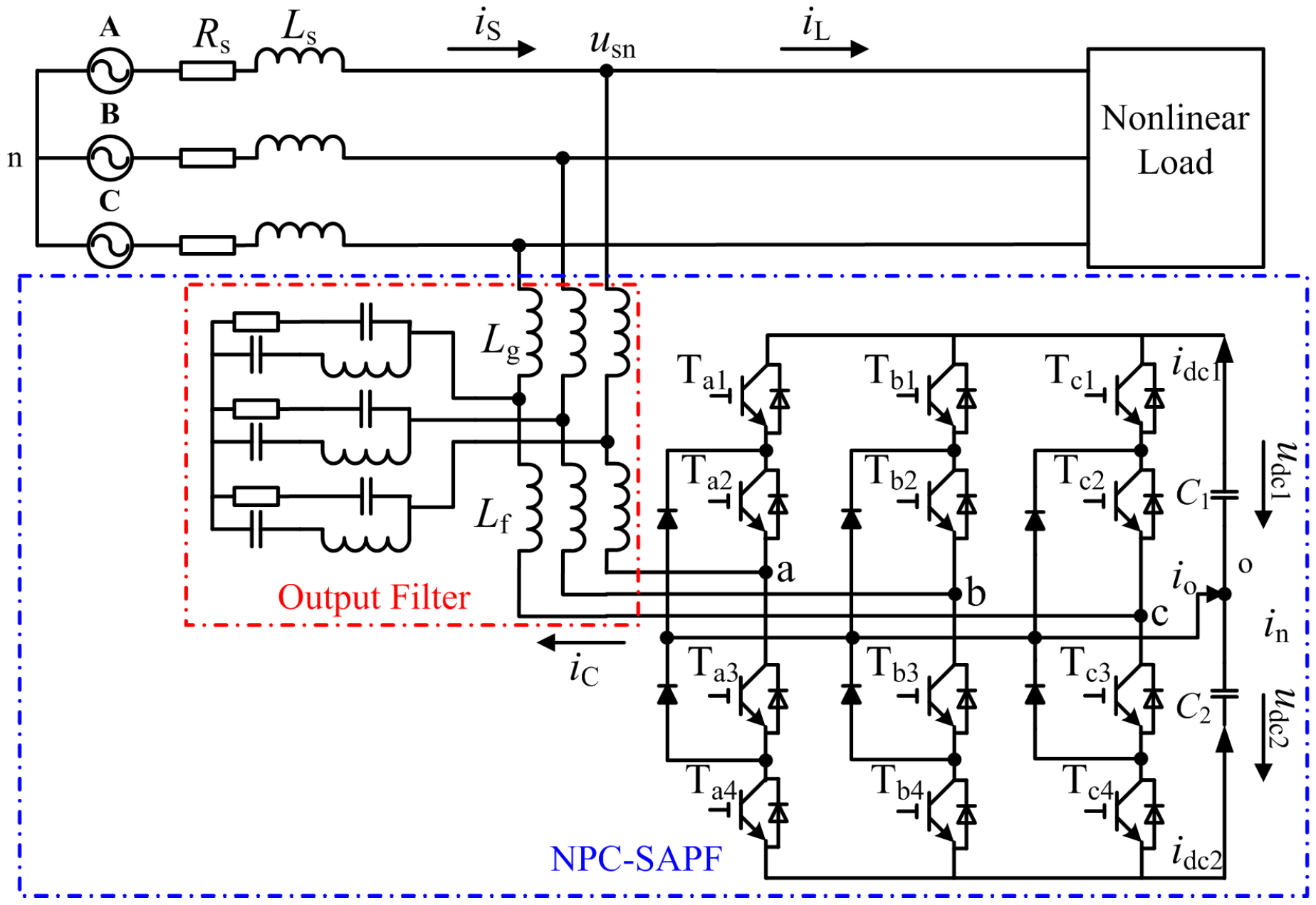
2. Mathematical Model

The configuration of NPC-SAPF is shown in Figure 1. The simulation and experimental system consist of three phase grid voltages with grid impedance, nonlinear load and NPC-SAPF. We take one phase as an example to define the variables. R_s and L_s are the grid equivalent resistor and inductor. i_S is the grid current. i_L is the load current. i_C is the output current. u_sn is the point of common coupling (PCC) voltage. L_g is the grid side inductor of the output filter. L_f is the inverter side inductor of the output filter. C₁ is the upper DC-capacitor. C₂ is the lower DC-capacitor. u_dc1 and u_dc2 are the voltages of C₁ and C₂, while i_dc1 and i_dc2 are the currents of C₁ and C₂.

According to Kirchhoff’s laws, the relationship between voltage and current can be deduced as follows:

$$\{\begin{array}{l}{L}_{\mathrm{T}}\frac{d{i}_{\mathrm{ca}}}{dt}=u_{\mathrm{asn}}-R_{\mathrm{f}}{i}_{\mathrm{ca}}-u_{\mathrm{ao}}-u_{\mathrm{on}}\\ L_{\mathrm{T}}\frac{d{i}_{\mathrm{cb}}}{dt}=u_{\mathrm{bsn}}-R_{\mathrm{f}}{i}_{\mathrm{cb}}-u_{\mathrm{bo}}-u_{\mathrm{on}}\\ L_{\mathrm{T}}\frac{d{i}_{\mathrm{cc}}}{dt}=u_{\mathrm{csn}}-R_{\mathrm{f}}{i}_{\mathrm{cc}}-u_{\mathrm{co}}-u_{\mathrm{on}}\\ C_{\mathrm{d}}\frac{d{u}_{\mathrm{dc}1}}{dt}=i_{\mathrm{dc}1}\\ C_{\mathrm{d}}\frac{d{u}_{\mathrm{dc}2}}{dt}=i_{\mathrm{dc}2}\end{array}$$

(1)

where u_asn, u_bsn and u_csn are three phase PCC voltages. i_ca, i_cb and i_cc are three phase output currents. u_ao, u_bo and u_co are voltages between nodes a, b, c to node o, respectively. u_on is the voltage between nodes o and n. L_T can be equivalent to the sum of L_f and L_g in the useful frequency range (50 Hz–2.5 kHz), which will be explained later. R_f is the line resistance of inductor L_f and C₁ = C₂ = C_d. The u_on meets Equation (2) because there is no zero sequence voltage, that is:

$$u_{\mathrm{on}}=-\frac{1}{3}(u_{\mathrm{ao}}+u_{\mathrm{bo}}+u_{\mathrm{co}})$$

(2)

The switching state of NPC-SAPF only includes three conditions, since only two IGBTs are on-state at the same time, i.e., T_x1 and T_x2 (x = a, b, c) are on-state, T_x2 and T_x3 are on-state or T_x3 and T_x4 are on-state, so the switching functions are defined as follows:

$$\begin{array}{l}{S}_{x1}=\{\begin{array}{ll}1& {\mathrm{T}}_{x1} \mathrm{and} {\mathrm{T}}_{x2} \mathrm{are} \text{on-state}\\ 0& {\mathrm{T}}_{x2} \mathrm{and} {\mathrm{T}}_{x3} \mathrm{are} \text{on-state} \mathrm{or} {\mathrm{T}}_{x3} \mathrm{and} {\mathrm{T}}_{x4} \mathrm{are} \text{on-state}\end{array}\\ S_{x2}=\{\begin{array}{ll}1& {\mathrm{T}}_{x3} \mathrm{and} {\mathrm{T}}_{x4} \mathrm{are} \text{on-state}\\ 0& {\mathrm{T}}_{x1} \mathrm{and} {\mathrm{T}}_{x2} \mathrm{are} \text{on-state} \mathrm{or} {\mathrm{T}}_{x2} \mathrm{and} {\mathrm{T}}_{x3} \mathrm{are} \text{on-state}\end{array}\end{array}$$

(3)

Thus, the relevant expressions are described as:

$$\{\begin{array}{l}{u}_{x\mathrm{o}}=S_{x1}{u}_{\mathrm{dc}1}-S_{x2}{u}_{\mathrm{dc}2}\\ i_{\mathrm{dc}1}=S_{\mathrm{a}1}{i}_{\mathrm{ca}}+S_{\mathrm{b}1}{i}_{\mathrm{cb}}+S_{\mathrm{c}1}{i}_{\mathrm{cc}}\\ i_{\mathrm{dc}2}=-(S_{\mathrm{a}2}{i}_{\mathrm{ca}}+S_{\mathrm{b}2}{i}_{\mathrm{cb}}+S_{\mathrm{c}2}{i}_{\mathrm{cc}})\end{array}$$

(4)

Combining Equations (1)–(4), the mathematical expressions can be obtained as follows:

$$\{\begin{array}{l}{L}_{\mathrm{T}}\left[\begin{array}{l}\frac{d{i}_{\mathrm{ca}}}{dt}\\ \frac{d{i}_{\mathrm{cb}}}{dt}\\ \frac{d{i}_{\mathrm{cc}}}{dt}\end{array}\right]=\left[\begin{array}{l}{u}_{\mathrm{asn}}\\ u_{\mathrm{bsn}}\\ u_{\mathrm{csn}}\end{array}\right]-R_{\mathrm{f}}\left[\begin{array}{l}{i}_{\mathrm{ca}}\\ i_{\mathrm{cb}}\\ i_{\mathrm{cc}}\end{array}\right]-\mathrm{M}\left\{\left[\begin{array}{l}{S}_{\mathrm{a}1}\\ S_{\mathrm{b}1}\\ S_{\mathrm{c}1}\end{array}\right]u_{\mathrm{dc}1}-\left[\begin{array}{l}{S}_{\mathrm{a}2}\\ S_{\mathrm{b}2}\\ S_{\mathrm{c}2}\end{array}\right]u_{\mathrm{dc}2}\right\}\\ C_{\mathrm{d}}\left[\begin{array}{l}\frac{d{u}_{\mathrm{dc}1}}{dt}\\ \frac{d{u}_{\mathrm{dc}2}}{dt}\end{array}\right]=\left[\begin{array}{l}\begin{array}{ccc}{S}_{\mathrm{a}1}& S_{\mathrm{b}1}& S_{\mathrm{c}1}\end{array}\\ \begin{array}{ccc}-S_{\mathrm{a}2}& -S_{\mathrm{b}2}& -S_{\mathrm{c}2}\end{array}\end{array}\right]\left[\begin{array}{l}{i}_{\mathrm{ca}}\\ i_{\mathrm{cb}}\\ i_{\mathrm{cc}}\end{array}\right]\end{array}$$

(5)

where the matrix M is:

$$\mathbf{M}=\frac{1}{3}\left[\begin{array}{l}\begin{array}{ccc}2& -1& -1\end{array}\\ \begin{array}{ccc}-1& 2& -1\end{array}\\ \begin{array}{ccc}-1& -1& 2\end{array}\end{array}\right]$$

(6)

Equation (5) should be simplified because M is too complicated for digital implementation. Let:

$$\left[\begin{array}{l}{D}_{aj}\\ D_{bj}\\ D_{cj}\end{array}\right]=\frac{1}{3}\left[\begin{array}{l}\begin{array}{ccc}2& -1& -1\end{array}\\ \begin{array}{ccc}-1& 2& -1\end{array}\\ \begin{array}{ccc}-1& -1& 2\end{array}\end{array}\right]\left[\begin{array}{l}{S}_{aj}\\ S_{bj}\\ S_{cj}\end{array}\right]$$

(7)

where j = 1, 2. Equation (7) can be equivalent to:

$$\{\begin{array}{l}{S}_{aj}-S_{bj}=D_{aj}-D_{bj}\\ S_{bj}-S_{cj}=D_{bj}-D_{cj}\end{array}$$

(8)

Because M is a singular matrix, (7) and (8) can be replaced by its dual solution (9):

$$\{\begin{array}{l}{S}_{aj}=D_{aj}\\ S_{bj}=D_{bj}\\ S_{cj}=D_{cj}\end{array}$$

(9)

The mathematical expressions of NPC-SAPF in three-phase coordinate are as follows:

$$\{\begin{array}{l}\frac{d{i}_{\mathrm{ca}}}{dt}=-\frac{R_{\mathrm{f}}}{L_{\mathrm{T}}}{i}_{\mathrm{ca}}-D_{\mathrm{a}1}{u}_{\mathrm{dc}1}+D_{\mathrm{a}2}{u}_{\mathrm{dc}2}+u_{\mathrm{asn}}\\ \frac{d{i}_{\mathrm{cb}}}{dt}=-\frac{R_{\mathrm{f}}}{L_{\mathrm{T}}}{i}_{\mathrm{cb}}-D_{\mathrm{b}1}{u}_{\mathrm{dc}1}+D_{\mathrm{b}2}{u}_{\mathrm{dc}2}+u_{\mathrm{bsn}}\\ \frac{d{i}_{\mathrm{cc}}}{dt}=-\frac{R_{\mathrm{f}}}{L_{\mathrm{T}}}{i}_{\mathrm{cc}}-D_{\mathrm{c}1}{u}_{\mathrm{dc}1}+D_{\mathrm{c}2}{u}_{\mathrm{dc}2}+u_{\mathrm{csn}}\\ \frac{d{u}_{\mathrm{dc}1}}{dt}=\frac{1}{C_{\mathrm{d}}}(D_{\mathrm{a}1}{i}_{\mathrm{ca}}+D_{\mathrm{b}1}{i}_{\mathrm{cb}}+D_{\mathrm{c}1}{i}_{\mathrm{cc}})\\ \frac{d{u}_{\mathrm{dc}2}}{dt}=\frac{-1}{C_{\mathrm{d}}}(D_{\mathrm{a}2}{i}_{\mathrm{ca}}+D_{\mathrm{b}2}{i}_{\mathrm{cb}}+D_{\mathrm{c}2}{i}_{\mathrm{cc}})\end{array}$$

(10)

In order to reduce the computing time and regulate the DC voltage, Equation (10) are transformed into SRF by Park transformation. The transformed expressions are as follows:

$$\{\begin{array}{l}\frac{d{i}_{\mathrm{cd}}}{dt}=\frac{1}{L_{\mathrm{T}}}(u_{\mathrm{dsn}}-D_{\mathrm{d}1}{u}_{\mathrm{dc}1}+D_{\mathrm{d}2}{u}_{\mathrm{dc}2}-R_{\mathrm{f}}{i}_{\mathrm{cd}}+\mathsf{\omega }{L}_{\mathrm{T}}{i}_{\mathrm{cq}})\\ \frac{d{i}_{\mathrm{cq}}}{dt}=\frac{1}{L_{\mathrm{T}}}(u_{\mathrm{qsn}}-D_{\mathrm{d}1}{u}_{\mathrm{dc}1}+D_{\mathrm{d}2}{u}_{\mathrm{dc}2}-R_{\mathrm{f}}{i}_{\mathrm{cq}}-\mathsf{\omega }{L}_{\mathrm{T}}{i}_{\mathrm{cd}})\\ \frac{d{u}_{\mathrm{dc}1}}{dt}=\frac{1}{C_{\mathrm{d}}}(D_{\mathrm{d}1}{i}_{\mathrm{cd}}+D_{\mathrm{q}1}{i}_{\mathrm{cq}})\\ \frac{d{u}_{\mathrm{dc}2}}{dt}=\frac{-1}{C_{\mathrm{d}}}(D_{\mathrm{d}2}{i}_{\mathrm{cd}}+D_{\mathrm{q}2}{i}_{\mathrm{cq}})\end{array}$$

(11)

where u_dsn, u_qsn are the PCC voltages in SRF. i_cd and i_cq are the output currents in SRF. D_d1 and D_q1, D_d2 and D_q2 are the upper and lower switching functions in SRF. ω is the grid fundamental angular frequency.

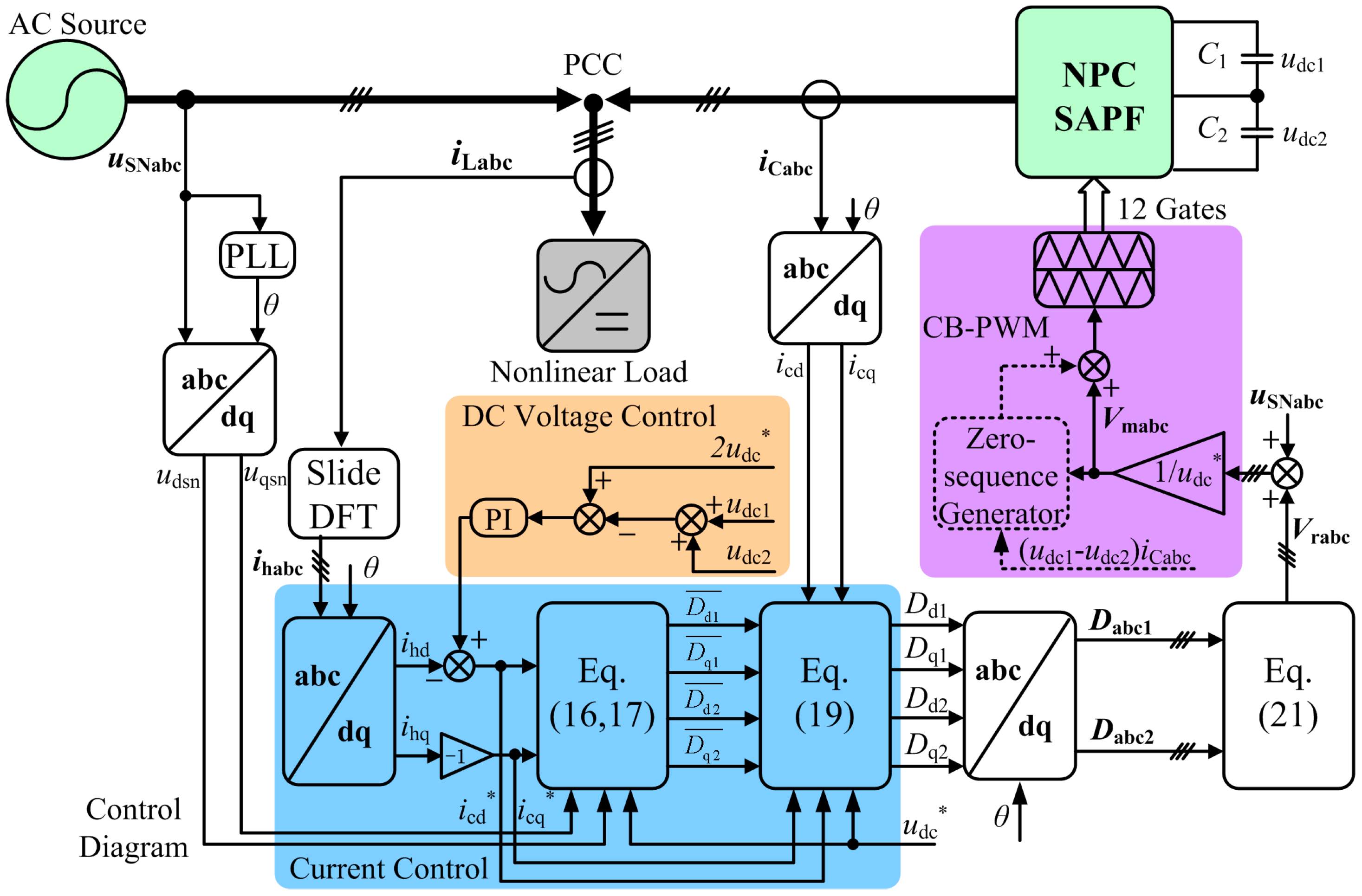
3. Lyapunov Stability Theory-Based Control Strategy

Lyapunov stability theory is based on the concept of equilibrium point stability. We choose the state variable: x₁ = i_cd − $i_{\mathrm{cd}}^{*}$, x₂ = i_cq − $i_{\mathrm{cq}}^{*}$, x₃ = u_dc1 − $u_{\mathrm{dc}1}^{*}$, x₄ = u_dc2 − $u_{\mathrm{dc}2}^{*}$. The block diagram of the proposed control strategy is shown in Figure 2.

In Figure 2, u_SNabc represents three phase PCC voltages. θ is the phase of PCC voltages, which is estimated from the phase lock loop (PLL). i_Labc represents three phase load currents. i_habc represents three phase harmonic currents. i_Cabc represents three phase output currents. $i_{\mathrm{cd}}^{*}$ and $i_{\mathrm{cq}}^{*}$ are extracted from i_Labc by slide discrete Fourier transformation (DFT) in SRF. $u_{\mathrm{dc}1}^{*}$ and $u_{\mathrm{dc}2}^{*}$ are the upper and lower DC-capacitor reference voltages ($u_{\mathrm{dc}1}^{*}$ = $u_{\mathrm{dc}2}^{*}$ = $u_{\mathrm{dc}}^{*}$ = 400 V in this paper).

3.1. Current Control Realization

According to Lyapunov stability theory, a nonlinear system is globally asymptotically stable if the Lyapunov candidate function F(x, t) satisfies the following properties [18,19,20]:

$$\{\begin{array}{ll}F(0,t)=0& \\ F(x,t)>0,& x\ne 0\\ \stackrel{•}{F}(x,t)<0,& x\ne 0\\ F(x,t)\to \infty ,& \Vert x\Vert \to \infty \end{array}$$

(12)

According to the first two properties in Equation (12), we choose F(x, t) as:

$$F(x,t)=\frac{1}{2}{L}_{\mathrm{T}}{x}_1^2+\frac{1}{2}{L}_{\mathrm{T}}{x}_2^2+\frac{1}{2}{C}_{\mathrm{d}}{x}_3^2+\frac{1}{2}{C}_{\mathrm{d}}{x}_4^2$$

(13)

The first-order partial derivative of F(x, t) is:

$$\frac{dF(x,t)}{dt}=L_{\mathrm{T}}{x}_1\frac{d{x}_1}{dt}+L_{\mathrm{T}}{x}_2\frac{d{x}_2}{dt}+C_{\mathrm{d}}{x}_3\frac{d{x}_3}{dt}+C_{\mathrm{d}}{x}_4\frac{d{x}_4}{dt}$$

(14)

Substituting state variables x₁, x₂, x₃, x₄ into Equation (11), the final state equations of NPC-SAPF are obtained as follows:

$$\{\begin{array}{l}\frac{d{x}_1}{dt}=\frac{1}{L_{\mathrm{T}}}(-D_{\mathrm{d}1}(x_3+u_{\mathrm{dc}1}^{*})+D_{\mathrm{d}2}(x_4+u_{\mathrm{dc}2}^{*})-R_{\mathrm{f}}{x}_1+\mathsf{\omega }{L}_{\mathrm{T}}{x}_2)+\frac{u_{\mathrm{dc}}^{*}}{L_{\mathrm{T}}}(\overline{D_{\mathrm{d}1}}-\overline{D_{\mathrm{d}2}})\\ \frac{d{x}_2}{dt}=\frac{1}{L_{\mathrm{T}}}(-D_{\mathrm{q}1}(x_3+u_{\mathrm{dc}1}^{*})+D_{\mathrm{q}2}(x_4+u_{\mathrm{dc}2}^{*})-R_{\mathrm{f}}{x}_2-\mathsf{\omega }{L}_{\mathrm{T}}{x}_1)+\frac{u_{\mathrm{dc}}^{*}}{L_{\mathrm{T}}}(\overline{D_{\mathrm{q}1}}-\overline{D_{\mathrm{q}2}})\\ \frac{d{x}_3}{dt}=\frac{1}{C_{\mathrm{d}}}(D_{\mathrm{d}1}(x_1+i_{\mathrm{cd}}^{*})+D_{\mathrm{q}1}(x_2+i_{\mathrm{cq}}^{*})-\overline{D_{\mathrm{d}1}}{i}_{\mathrm{cd}}^{*}-\overline{D_{\mathrm{q}1}}{i}_{\mathrm{cq}}^{*})\\ \frac{d{x}_4}{dt}=\frac{-1}{C_{\mathrm{d}}}(D_{\mathrm{d}2}(x_1+i_{\mathrm{cd}}^{*})+D_{\mathrm{q}2}(x_2+i_{\mathrm{cq}}^{*})-\overline{D_{\mathrm{d}2}}{i}_{\mathrm{cd}}^{*}-\overline{D_{\mathrm{q}2}}{i}_{\mathrm{cq}}^{*})\end{array}$$

(15)

where $\overline{D_{\mathrm{d}1}}$, $\overline{D_{\mathrm{d}2}}$, $\overline{D_{\mathrm{q}1}}$ and $\overline{D_{\mathrm{q}2}}$ are steady-state switching functions. According to Equation (11), we can obtain the following steady-state switching expressions:

$$\{\begin{array}{l}\overline{D_{\mathrm{d}1}}-\overline{D_{\mathrm{d}2}}=\frac{1}{u_{\mathrm{dc}}^{*}}(u_{\mathrm{dsn}}-R_{\mathrm{f}}{i}_{\mathrm{cd}}^{*}+\mathsf{\omega }{L}_{\mathrm{T}}{i}_{\mathrm{cq}}^{*}-L_{\mathrm{T}}\frac{d{i}_{\mathrm{cd}}^{*}}{dt})\\ \overline{D_{\mathrm{q}1}}-\overline{D_{\mathrm{q}2}}=\frac{1}{u_{\mathrm{dc}}^{*}}(u_{\mathrm{qsn}}-R_{\mathrm{f}}{i}_{\mathrm{cq}}^{*}-\mathsf{\omega }{L}_{\mathrm{T}}{i}_{\mathrm{cd}}^{*}-L_{\mathrm{T}}\frac{d{i}_{\mathrm{cq}}^{*}}{dt})\\ \frac{d{u}_{\mathrm{dc}1}^{*}}{dt}=\frac{1}{C_{\mathrm{d}}}(\overline{D_{\mathrm{d}1}}{i}_{\mathrm{cd}}^{*}+\overline{D_{\mathrm{q}1}}{i}_{\mathrm{cq}}^{*})\\ \frac{d{u}_{\mathrm{dc}2}^{*}}{dt}=\frac{-1}{C_{\mathrm{d}}}(\overline{D_{\mathrm{d}2}}{i}_{\mathrm{cd}}^{*}+\overline{D_{\mathrm{q}2}}{i}_{\mathrm{cq}}^{*})\end{array}$$

(16)

In order to maintain the symmetry of two switching functions, the steady-state switching functions are chosen as:

$$\{\begin{array}{l}\overline{D_{\mathrm{d}1}}=0.5(\overline{D_{\mathrm{d}1}}-\overline{D_{\mathrm{d}2}})\\ \overline{D_{\mathrm{d}2}}=-0.5(\overline{D_{\mathrm{d}1}}-\overline{D_{\mathrm{d}2}})\\ \overline{D_{\mathrm{q}1}}=0.5(\overline{D_{\mathrm{q}1}}-\overline{D_{\mathrm{q}2}})\\ \overline{D_{\mathrm{q}2}}=-0.5(\overline{D_{\mathrm{q}1}}-\overline{D_{\mathrm{q}2}})\end{array}$$

(17)

The first-order partial derivative of F(x, t) is deduced by Equations (14)–(17), i.e.,:

$$\begin{array}{c}\frac{dF(x,t)}{dt}=-R_{\mathrm{f}}(x_1^2+x_2^2)+(D_{\mathrm{d}1}-\overline{D_{\mathrm{d}1}})(x_3{i}_{\mathrm{cd}}^{*}-x_1{u}_{\mathrm{dc}}^{*})+(D_{\mathrm{d}2}-\overline{D_{\mathrm{d}2}})(x_1{u}_{\mathrm{dc}}^{*}-x_4{i}_{\mathrm{cd}}^{*})\\ +(D_{\mathrm{q}1}-\overline{D_{\mathrm{q}1}})(x_3{i}_{\mathrm{cq}}^{*}-x_2{u}_{\mathrm{dc}}^{*})+(D_{\mathrm{q}2}-\overline{D_{\mathrm{q}2}})(x_2{u}_{\mathrm{dc}}^{*}-x_4{i}_{\mathrm{cq}}^{*})\end{array}$$

(18)

It is clear that the first term of Equation (18) is always negative. In order to meet the last two properties in Equation (12), the switching functions are chosen as:

$$\{\begin{array}{l}{D}_{\mathrm{d}1}=\overline{D_{\mathrm{d}1}}+{\mathsf{\lambda }}_1(x_3{i}_{\mathrm{cd}}^{*}-x_1{u}_{\mathrm{dc}}^{*})\\ D_{\mathrm{q}1}=\overline{D_{\mathrm{q}1}}+{\mathsf{\lambda }}_1(x_3{i}_{\mathrm{cq}}^{*}-x_2{u}_{\mathrm{dc}}^{*})\\ D_{\mathrm{d}2}=\overline{D_{\mathrm{d}2}}+{\mathsf{\lambda }}_2(x_1{u}_{\mathrm{dc}}^{*}-x_4{i}_{\mathrm{cd}}^{*})\\ D_{\mathrm{q}2}=\overline{D_{\mathrm{q}2}}+{\mathsf{\lambda }}_2(x_2{u}_{\mathrm{dc}}^{*}-x_4{i}_{\mathrm{cq}}^{*})\end{array}\begin{array}{cc}\mathrm{with}& {\mathsf{\lambda }}_1,{\mathsf{\lambda }}_2< 0\end{array}$$

(19)

where λ₁, λ₂ are the gains of the control strategy. Considering the symmetry of control strategy, λ₁ = λ₂ = λ is proposed. Finally, the switching functions D_a1, D_b1, D_c1; D_a2, D_b2, D_c2 in three-phase coordinate are obtained by the Park inverse transformation.

3.2. DC Voltage Control Realization

According to instantaneous reactive power theory, the total three-phase instantaneous reactive power of NPC-SAPF is zero. Thus the last two DC voltage expressions in Equation (11) are simplified as:

$$\frac{d(u_{\mathrm{dc}1}+u_{\mathrm{dc}2})}{dt}=\frac{1}{C_{\mathrm{d}}}(D_{\mathrm{d}1}-D_{\mathrm{d}2})i_{\mathrm{cd}}$$

(20)

The differential Equation (20) indicates that DC voltage control loop can be designed by integrating a suitable PI regulator and superposing it on the active current i_cd. The PI regulator can be designed as a second order optimal system [20].

3.3. NP Voltage Balance through PWM Realization

According to the first equation in Equation (4), the modulation voltage V_mabc is calculated as:

$$\{\begin{array}{l}{V}_{\mathrm{rabc}}=D_{\mathrm{abc}1}\frac{u_{\mathrm{dc}1}}{u_{\mathrm{dc}}^{*}}-D_{\mathrm{abc}2}\frac{u_{\mathrm{dc}2}}{u_{\mathrm{dc}}^{*}}\\ V_{\mathrm{mabc}}=\frac{V_{\mathrm{rabc}}+u_{\mathrm{SNabc}}}{u_{\mathrm{dc}}^{*}}\end{array}$$

(21)

where D_abc1 and D_abc2 are three phase switching functions.

An outstanding CB-PWM with zero-sequence voltage injection is introduced to keep the NP voltage balance [25]. The CB-PWM strategy achieves voltage-balancing task and reduces switching losses, compared with SVPWM.

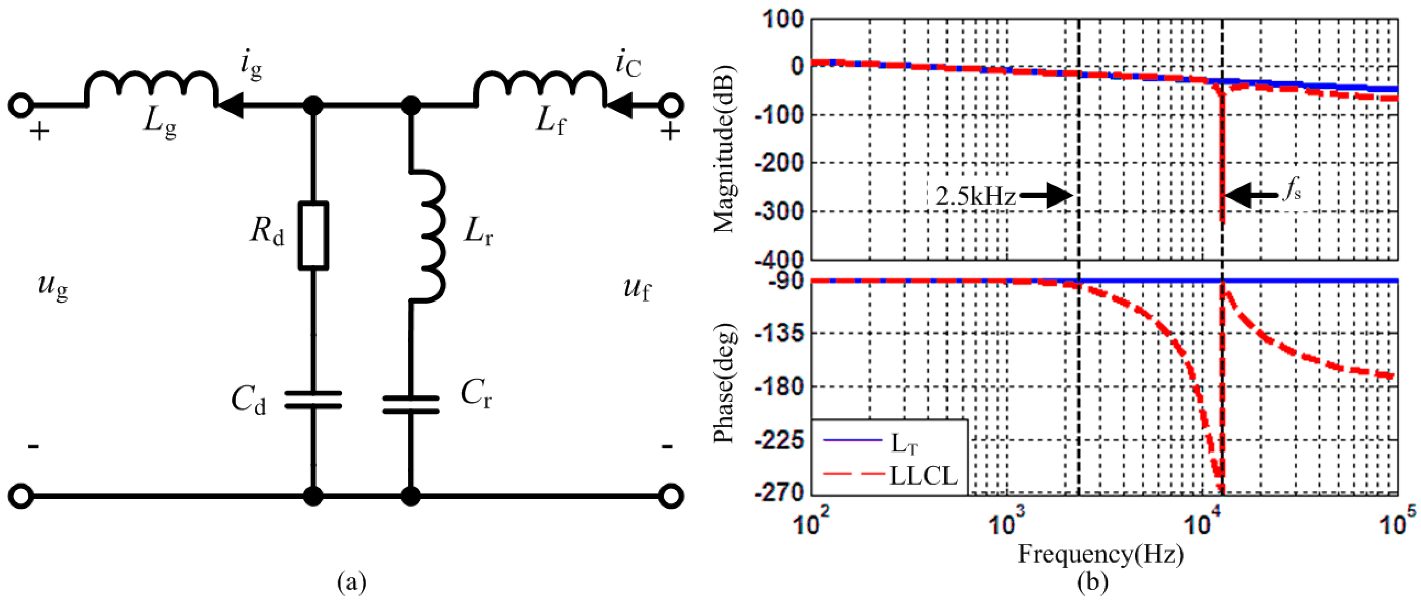
3.4. LCL Type Output Filter Design

The design criteria of LCL type filter when applied to NPC-SAPF are summarized as follows:

(1)

In order to ensure the output current follow the highest reference current change rate and limit the output current ripple. L_T should meet: $\frac{u_{\mathrm{dc}}^{*}}{8\Delta I_{\mathrm{C}}{f}_{\mathrm{s}}}\le L_{\mathrm{T}}\le \frac{u_{\mathrm{dc}}^{*}-1.1u_{\mathrm{SNm}}}{2M_{49}{\mathsf{\omega }}_{49}}$, where ΔI_c is the output current ripple. f_s is the switching frequency (12.8 kHz). u_SNm is the amplitude of grid phase voltage. M₄₉ is the 49th harmonic current amplitude which is chosen as 0.5 A. ω₄₉ is the 49th harmonic angular frequency.

(2)

L_r and C_r resonates at f_s: $L_{\mathrm{r}}{C}_{\mathrm{r}}=\frac{1}{4{\mathsf{\pi }}^2{f}_{\mathrm{s}}^2}$.

(3)

In order to obtain good high frequency attenuate rate and appropriate output bandwidth for NPC-SAPF, L_f, L_g and C_a should meet: L_f ≥ 5L_g and $f_{\mathrm{m}}\le \frac{1}{2\mathsf{\pi }}\sqrt{\frac{L_{\mathrm{g}}+L_{\mathrm{f}}}{L_{\mathrm{g}}{L}_{\mathrm{f}}{C}_{\mathrm{a}}}}\le \frac{1}{2}{f}_{\mathrm{s}}$, where f_m is the highest compensated frequency (2.5 kHz). C_a = C_d + C_r.

(4)

Larger C_d/C_r is helpful to improve the damping performance but increase the power losses [29]. Considering the harmonics characteristics of NPC-SAPF, C_d/C_r = 8 and R_d = 3 are proposed.

The detailed values of LLCL filter are shown in Section 5. The single structure and the Bode plots of i_g(s)/u_f(s) are shown in Figure 3.

In Figure 3, it can be seen that the LLCL filter has only one tuned trap at switching frequency f_s, which indicates it can eliminate the switching harmonic currents effectively. Moreover, the characteristics of single L_T and LLCL filter below 2.5 kHz are almost same. Thus the mathematical model of LLCL filter can be instead by L_T (L_T = L_g + L_f) in the useful frequency range (50 Hz–2.5 kHz).

4. Comparison Analysis of System Stability

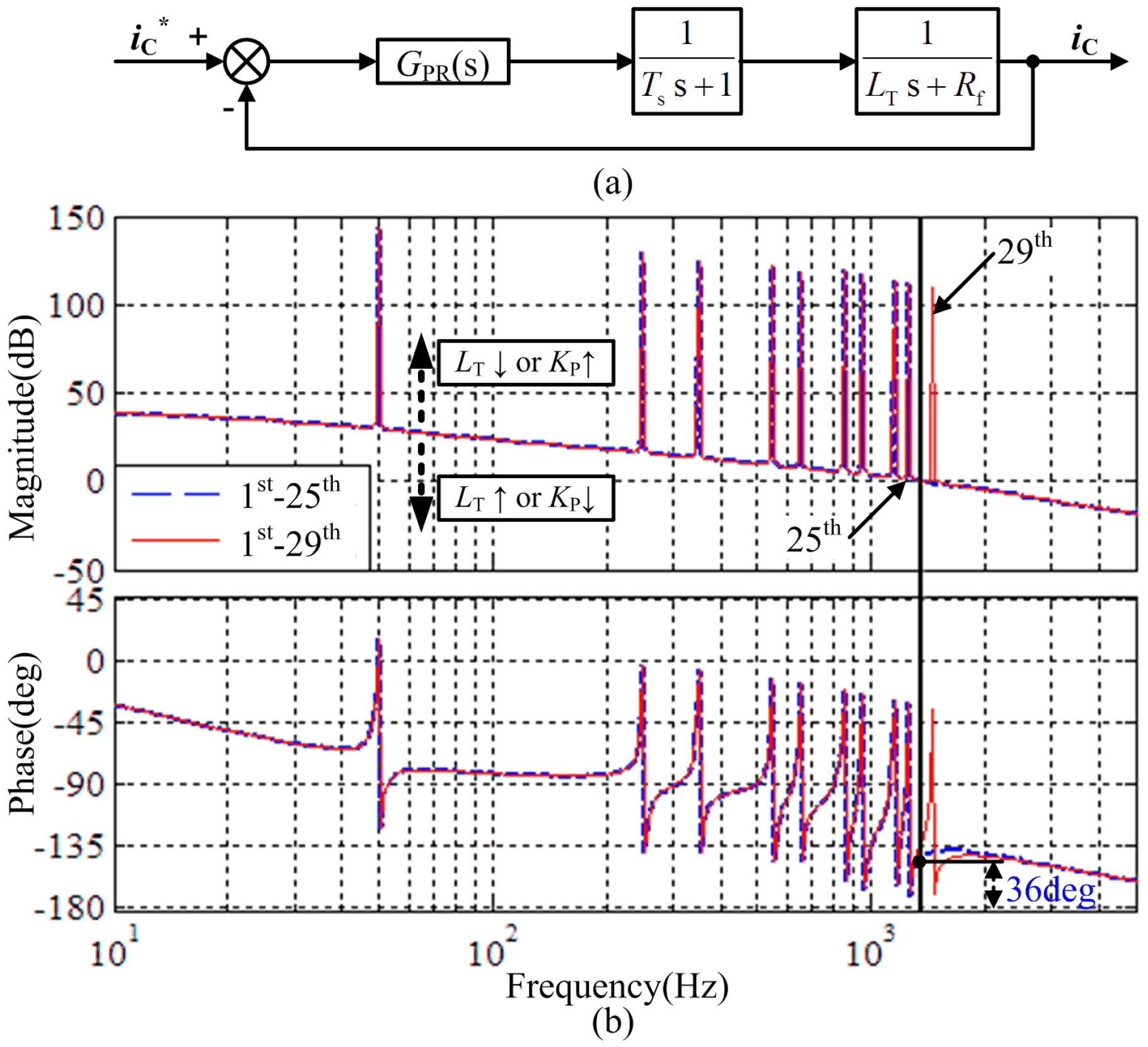
4.1. Stability of the Classical Feedback Control Strategy

PR and vector PI (VPI) controllers are effective and popular methods for SAPF, and their systematic design methods are described in [3,13]. As they have similar filtering properties on each specified frequency [3], we take PR controllers as an analysis object. The current controllers G_PR(s) take the form:

$$G_{\mathrm{P}\mathrm{R}}(\mathrm{s})=K_{\mathrm{P}}+{\displaystyle \sum _{k=1,5,7\cdots }^n{K}_{{\mathrm{I}}_k}\frac{\mathrm{s}}{{\mathrm{s}}^2+{\mathsf{\omega }}_k^2}}$$

(22)

where k = 6i ± 1, and i = 1, 2, 3, 4. According to [3], K_P = 2.5, K_I5 = K_I7 = 256, K_I11 = K_I13 = 128, K_I17 = K_I19 = 64, K_I23 = K_I25 = 32 are used in this paper. The closed-loop current control model and open-loop bode plots are shown in Figure 4.

It can be seen that the phase margin results in 36° when the PR controllers (G_PR(s)) order is below 29th (blue dotted line in Figure 4b), which assures system stability. When a 29th or higher frequency resonant controller (red solid line in Figure 4b) is added, the magnitude is below zero, which indicates the phase margin is not enough. This condition may be unstable or even resonate above 29th harmonics. This unstable situation will be solved by decreasing L_T or increasing K_P, but the current ripple will be too big for output current waveform, so PR controllers cannot compensate high-frequency harmonics stably.

4.2. The Proposed Control Strategy Stability

When the control system has the following state-space form:

$$\{\begin{array}{l}\frac{dx}{dt}=Ax+Bu\\ y=Cx+Du\end{array}$$

(23)

The characteristic equation is obtained by |sI − A|. And the relevant deduction is described in Appendix. Let f(s, λ) = |sI − A|. The three-dimensional plot of f(s, λ) is shown in Figure 5. The system is globally stable when all eigenvalues are in the left-half plane. Thus, λ value should follow the trend of the red dotted line in Figure 5. The choice of λ is based on the fast response of the system and good quality of compensation. It is worth noting that the system achieves better dynamic performance when λ is closer to the origin point but better steady-state performance when λ is far away from the origin point.

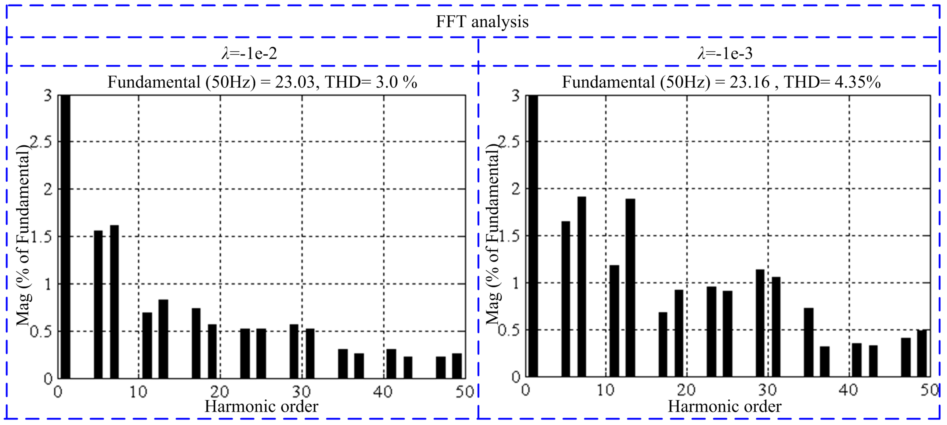
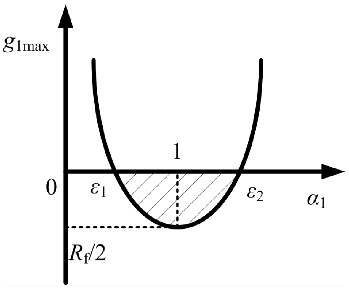
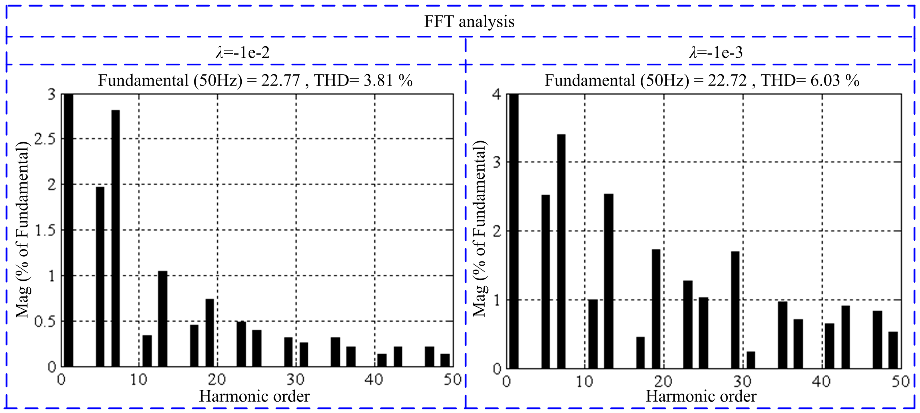
4.3. Tolerance of Inaccurate Model on Stability

The precision of the proposed control strategy depends on the differences between mathematical model and real plant. From the mathematical model, it can be seen that the mathematical model will deviate from real plant when the reference values do not match with the actual one. This condition means the partial derivative of F(x, t) may not be negative [32]. Thus, we assume that the expected values are (I_cd, I_cq, U_dc), the adopted values are ($I_{\mathrm{cd}}^{\prime }$, $I_{\mathrm{cq}}^{\prime }$, $U_{\mathrm{dc}}^{\prime }$). Therefore, Equation (18) can be deduced as:

$$\begin{array}{cc}\hfill \frac{dF(x,t)}{dt}=& -R_{\mathrm{f}}(x_1^2+x_2^2)+\Delta d_1(x_3{I}_{\mathrm{cd}}-x_1{U}_{\mathrm{dc}})+\Delta q_1(x_3{I}_{\mathrm{cq}}-x_2{U}_{\mathrm{dc}})\hfill \\ & +\Delta d_2(x_1{U}_{\mathrm{dc}}-x_4{I}_{\mathrm{cd}})+\Delta q_2(x_2{U}_{\mathrm{dc}}-x_4{I}_{\mathrm{cq}})\hfill \\ \hfill =& -R_{\mathrm{f}}(x_1^2+x_2^2)+\Delta d_1{U}_{\mathrm{dc}}(x_3{I}_{\mathrm{cd}}/U_{\mathrm{dc}}-x_1)+\Delta q_1{U}_{\mathrm{dc}}(x_3{I}_{\mathrm{cq}}/U_{\mathrm{dc}}-x_2)\hfill \\ & +\Delta d_2{U}_{\mathrm{dc}}(x_1-x_4{I}_{\mathrm{cd}}/U_{\mathrm{dc}})+\Delta q_2{U}_{\mathrm{dc}}(x_2-x_4{I}_{\mathrm{cq}}/U_{\mathrm{dc}})\hfill \end{array}$$

(24)

where:

$$\{\begin{array}{l}\Delta d_1=\mathsf{\lambda }(x_3{I}_{\mathrm{cd}}^{\prime }-x_1{U}_{\mathrm{dc}}^{\prime })=\mathsf{\lambda }{U}_{\mathrm{dc}}^{\prime }(x_3{I}_{\mathrm{cd}}^{\prime }/U_{\mathrm{dc}}^{\prime }-x_1)\\ \Delta q_1=\mathsf{\lambda }(x_3{I}_{\mathrm{cd}}^{\prime }-x_2{U}_{\mathrm{dc}}^{\prime })=\mathsf{\lambda }{U}_{\mathrm{dc}}^{\prime }(x_3{I}_{\mathrm{cq}}^{\prime }/U_{\mathrm{dc}}^{\prime }-x_2)\\ \Delta d_2=\mathsf{\lambda }(x_1{U}_{\mathrm{dc}}^{\prime }-x_4{I}_{\mathrm{cd}}^{\prime })=\mathsf{\lambda }{U}_{\mathrm{dc}}^{\prime }(x_1-x_4{I}_{\mathrm{cd}}^{\prime }/U_{\mathrm{dc}}^{\prime })\\ \Delta q_2=\mathsf{\lambda }(x_2{U}_{\mathrm{dc}}^{\prime }-x_4{I}_{\mathrm{cq}}^{\prime })=\mathsf{\lambda }{U}_{\mathrm{dc}}^{\prime }(x_2-x_4{I}_{\mathrm{cq}}^{\prime }/U_{\mathrm{dc}})\end{array}$$

(25)

It can be figured out that if $I_{\mathrm{cd}}^{\prime }$/$U_{\mathrm{dc}}^{\prime }$ = I_cd/U_dc and $I_{cq}^{\prime }$/$U_{\mathrm{dc}}^{\prime }$ = I_cq/U_dc, Equation (24) will be negative. Let us define:

$$\begin{array}{l}{I}_{\mathrm{cd}}^{\prime }/U_{\mathrm{dc}}={\mathsf{\alpha }}_1{I}_{\mathrm{cd}}/U_{\mathrm{dc}},I_{\mathrm{cq}}^{\prime }/U_{\mathrm{dc}}={\mathsf{\alpha }}_2{I}_{\mathrm{cq}}/U_{\mathrm{dc}}\\ y_1=x_1/I_{\mathrm{cd}},y_2=x_2/I_{\mathrm{cq}},y_3=x_3/U_{\mathrm{dc}},y_4=x_4/U_{\mathrm{dc}}\end{array}$$

(26)

Then Equation (24) can be deduced by the adopted values in Equation (25):

$$\begin{array}{ll}\frac{dF(x,t)}{dt}& =I_{\mathrm{cd}}^2[\mathsf{\lambda }{U}_{\mathrm{dc}}{U}_{\mathrm{dc}}^{\prime }(y_3-y_1)({\mathsf{\alpha }}_1{y}_3-y_1)-R_{\mathrm{f}}/2y_1^2]\\ & I_{\mathrm{cq}}^2[\mathsf{\lambda }{U}_{\mathrm{dc}}{U}_{\mathrm{dc}}^{\prime }(y_3-y_2)({\mathsf{\alpha }}_2{y}_3-y_2)-R_{\mathrm{f}}/2y_2^2]\\ & I_{\mathrm{cd}}^2[\mathsf{\lambda }{U}_{\mathrm{dc}}{U}_{\mathrm{dc}}^{\prime }(y_4-y_1)({\mathsf{\alpha }}_1{y}_4-y_1)-R_{\mathrm{f}}/2y_1^2]\\ & I_{\mathrm{cq}}^2[\mathsf{\lambda }{U}_{\mathrm{dc}}{U}_{\mathrm{dc}}^{\prime }(y_4-y_2)({\mathsf{\alpha }}_2{y}_4-y_2)-R_{\mathrm{f}}/2y_2^2]\\ & =I_{\mathrm{cd}}^2{f}_1(y_1,y_3)+I_{\mathrm{cq}}^2{f}_2(y_2,y_3)+I_{\mathrm{cd}}^2{f}_3(y_1,y_4)+I_{\mathrm{cq}}^2{f}_4(y_2,y_4)\end{array}$$

(27)

It is clear that if f₁(y₁, y₃), f₂(y₂, y₃), f₃(y₁, y₄), f₄(y₂, y₄) are all below zero, Equation (27) will be negative. Let us take the first part in Equation (27) as an example, it is assumed that y₃ is equal to k·y₁, giving:

$$\begin{array}{l}{f}_1(y_1,y_3)=\mathsf{\lambda }{U}_{\mathrm{dc}}{U}_{\mathrm{dc}}^{\prime }(y_3-y_1)({\mathsf{\alpha }}_1{y}_3-y_1)-R_{\mathrm{f}}/2y_1^2\\ =y_1^2[\mathsf{\lambda }{U}_{\mathrm{dc}}{U}_{\mathrm{dc}}^{\prime }{\mathsf{\alpha }}_1{k}^2-\mathsf{\lambda }{U}_{\mathrm{dc}}{U}_{\mathrm{dc}}^{\prime }(1+{\mathsf{\alpha }}_1)k+(\mathsf{\lambda }{U}_{\mathrm{dc}}{U}_{\mathrm{dc}}^{\prime }-R_{\mathrm{f}}/2)]\\ =y_1^2{g}_1(\mathsf{\lambda },{\mathsf{\alpha }}_1,k)\end{array}$$

(28)

It is clear that g₁(λ, α₁, k) is a quadratic equation of k, and g₁(λ, α₁, k) has a maximum value at k_m = (1 + α₁)/(2α₁) given by:

$$g_{1\max }=\mathsf{\lambda }{U}_{\mathrm{dc}}{U}_{\mathrm{dc}}^{\prime }[1-{(1+{\mathsf{\alpha }}_1)}^2/4{\mathsf{\alpha }}_1]-R_{\mathrm{f}}/2$$

(29)

The error parameter α₁ will be given a value range when g_1max is below zero. The relationship between α₁ and g_1max is shown in Figure 6.

According to the dashed area in Figure 6 and for an expected range of uncertainty 1 − ε < α₁ < 1 + ε, the maximum value of λ can be calculated from Equation (29):

$${\mathsf{\lambda }}_{\max }=\frac{2R_{\mathrm{f}}\left(\mathsf{\epsilon }-1\right)}{U_{\mathrm{dc}}{U}_{\mathrm{dc}}^{\prime }{\mathsf{\epsilon }}^2}$$

(30)

where λ_max is the maximum of control gain, ε is the uncertainty range. For example, if an uncertainty range of ±5% is chosen, λ_max is calculated as −2.6 × 10⁻⁴.

5. Simulation Results

The proposed control strategy based on Lyapunov stability theory is simulated in MATLAB/Simulink. The main purpose of the simulation is to test three aspects of the control strategy: (1) The proposed control strategy can obtain wider output bandwidth than the closed-feedback control methods; (2) the proposed control strategy has a fast dynamic response for step-change of nonlinear load; (3) the proposed control strategy has a good steady-state harmonic compensation performance. The simulation parameter specifications are given in

Table 1. Simulation parameters.

Parameter	Value	Parameter	Value
uSNabc	220 V	Lf	0.45 mH
f0	50 Hz	Rf	0.05 Ω
fs	12.8 kHz	Lg	0.05 mH
$u_{\mathrm{dc}}^{*}$	400 V	Lr	70.28 μH
Ls	0.02 mH	Cr	2.2 μF
Rs	0.05 Ω	Cd	17.6 μF
C1(C2)	4650 μF	Rd	5 Ω

.

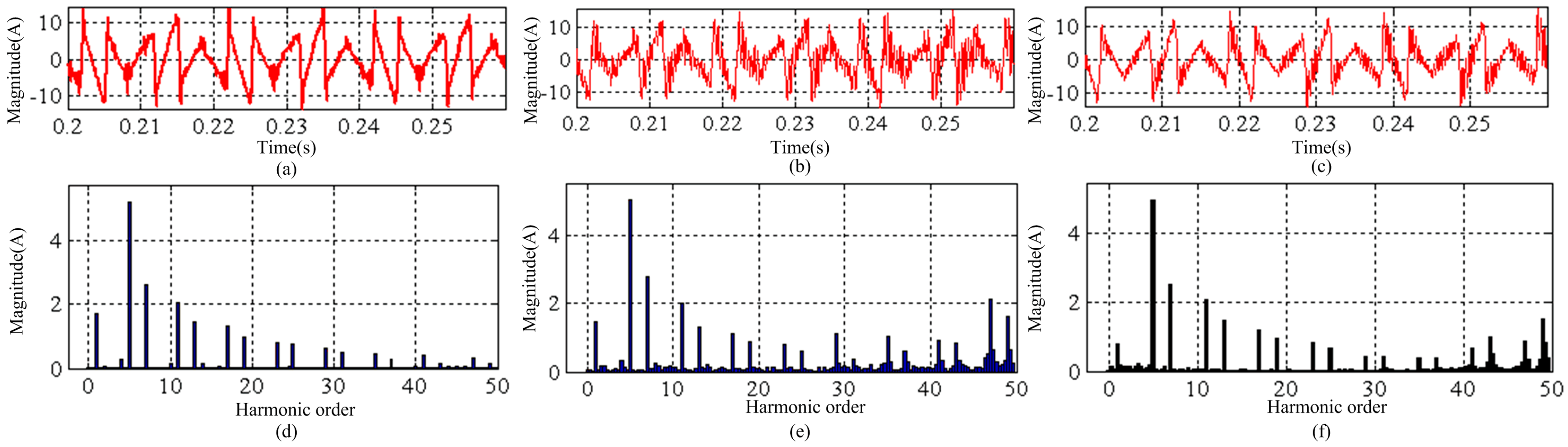
5.1. Comparisons between the Proposed Control Strategy and the Classical Feedback Control Methods

In order to verify the system stability analysis in Section 4, the proposed control strategy with λ = −1 × 10⁻², PR controllers and selective harmonics (VPI) controllers described in [3,13] are simulated. They all output 1st–50th harmonic currents. The simulation results are shown in Figure 7 and Figure 8.

It can be seen from Figure 7 that NPC-SAPF with the proposed control strategy outputs 1st–50th harmonic currents stably. The output current of NPC-SAPF by using PR controllers (1st–50th resonant controllers) resonates between the 29th and the 50th harmonics. While the output current of NPC-SAPF by using VPI controllers (1st–50th controllers) resonates between the 41st and the 50th harmonics. In Figure 8, when PR and VPI controllers only regulate harmonics below 25th, the resonant phenomenon disappears. Simulation results in Figure 7 and Figure 8 indicate that NPC-SAPF by using the proposed control method has wider output bandwidth than PR and VPI controllers.

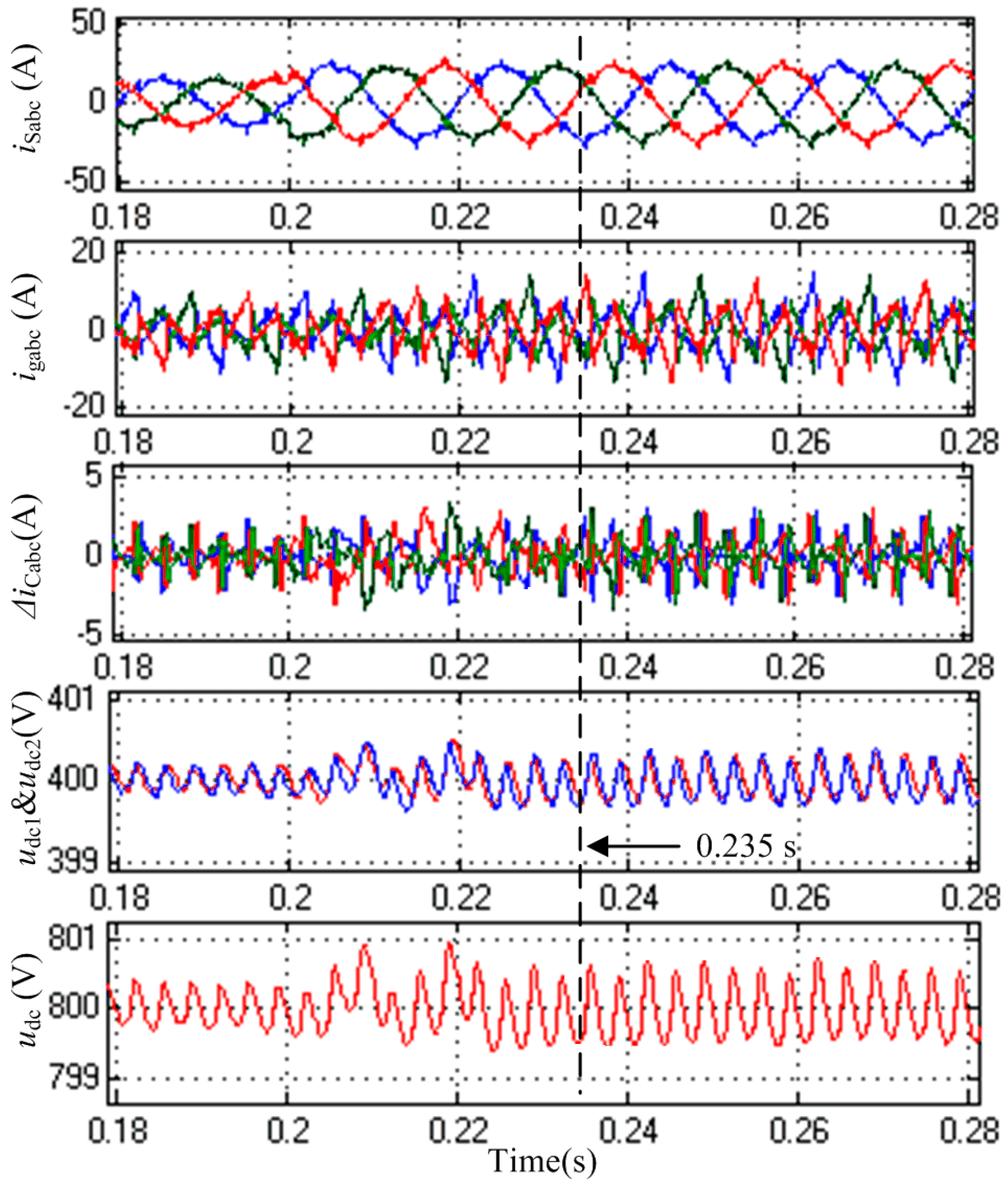
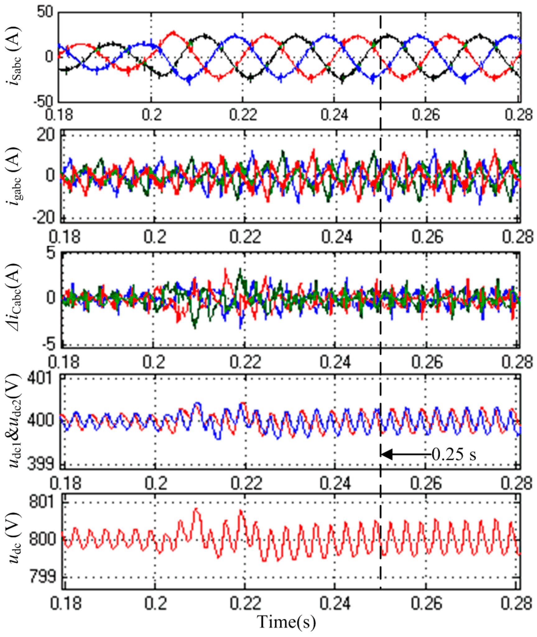
5.2. Dynamic Response of the NPC-SAPF

The waveforms of PCC voltages (u_SNabc) and nonlinear load currents (i_Labc) are shown in Figure 9. The nonlinear load is an uncontrolled rectifier bridge (URB) with inductors (0.9 mH) and step-change resistors (40 Ω → 25 Ω). Grid currents (i_Sabc), NPC-SAPF output currents on L_g (i_gabc), the difference between the reference currents and i_gabc (Δi_Cabc), upper and lower DC-capacitor voltages (u_dc1&u_dc2) and DC-link total voltage (u_dc) are depicted in the rest figures of simulation. The nonlinear load changes 40 Ω → 25 Ω at 0.2 s. Figure 10 and Figure 11 show the dynamic response of NPC-SAPF when λ = −1 × 10⁻² and λ = −1 × 10⁻³.

As shown in Figure 10 and Figure 11, the DC-link voltage is regulated at 800 V and the voltages of upper and lower DC-capacitors are balanced. The waveforms of i_Sabc when λ = −1 × 10⁻² are better than λ = −1 × 10⁻³. It can be found from the last two sub-figures in Figure 10 and Figure 11 that the settling time of λ = −1 × 10⁻² (50 ms) is longer than λ = −1 × 10⁻³ (35 ms). The simulation results agree well with the analysis in Section 4.2. It also can be seen that the overshoots of i_gabc and u_dc are very small. We can draw a conclusion from the simulation results that the NPC-SAPF can obtain fast dynamic response with small overshoot for a step-change of the nonlinear load.

5.3. Steady-State Performance of the NPC-SAPF

The NPC-SAPF operates stably after 0.25 s. The corresponding FFT analysis is shown in Figure 12. One can figure out that the THD of phase A grid current is decreased from 28.2% (22.61 A fundamental) to 3.81% and 6.03% when λ = −1 × 10⁻² and λ = −1 ×10⁻³, respectively. Moreover, the switching frequency (12.8 kHz) harmonic currents are eliminated effectively by the proposed LLCL filter. The THD when λ = −1 × 10⁻³ cannot satisfy the requirements of IEEE Standard 519-2014. The detailed simulation data when λ = −1 × 10⁻² are shown in

Table 2. Detailed simulation data.

Harmonic Order	Load Current		Grid Current		IEEE Standard 519-2014
	Amplitude (A)	Percent (%)	Amplitude (A)	Percent (%)	Maximum Percent (%)
1	22.61	100	22.77	100	100
5	5.11	22.59	0.45	1.97	4.0
7	2.45	10.85	0.64	2.81	4.0
11	1.94	8.60	0.08	0.34	2.0
13	1.28	5.67	0.24	1.04	2.0
17	1.10	4.87	0.10	0.45	1.5
19	0.78	3.46	0.17	0.74	1.5
23	0.69	3.06	0.11	0.48	0.6
25	0.50	2.20	0.09	0.39	0.6
29	0.45	1.98	0.07	0.31	0.6
31	0.32	1.40	0.06	0.26	0.6
35	0.29	1.29	0.07	0.31	0.3
37	0.20	0.87	0.05	0.21	0.3
41	0.19	0.85	0.03	0.13	0.3
43	0.12	0.53	0.05	0.21	0.3
47	0.13	0.60	0.06	0.26	0.3
49	0.07	0.32	0.03	0.13	0.3
THD (%)	28.20		3.81		5.0

. From Table 2, each harmonic content of grid current also reach the requirements of IEEE Standard 519-2014. Thus λ = −1 × 10⁻² is recommended.

It can be concluded from simulation results that the NPC-SAPF by using the proposed strategy has a wider output bandwidth on the premise of good dynamic response and satisfactory steady-state performance.

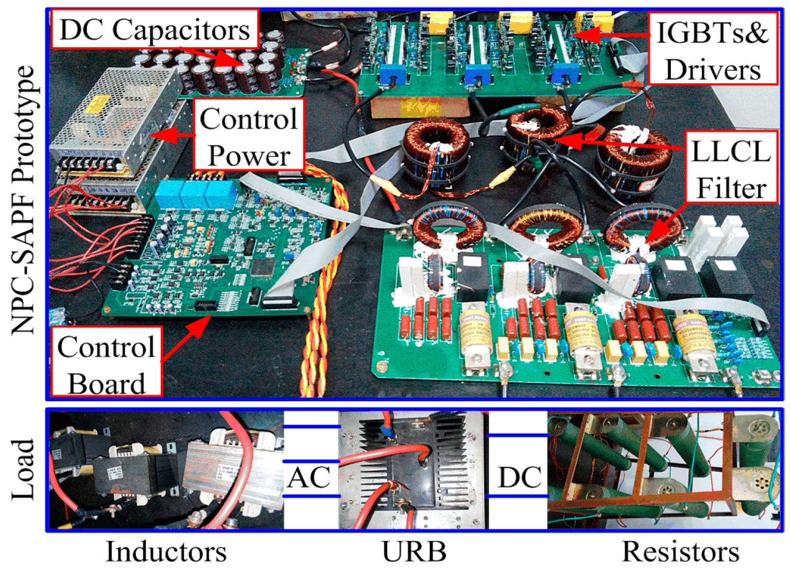
6. Experimental Results

The proposed control strategy is implemented on a 6.6 kVA NPC-SAPF laboratory prototype using the same simulation specifications given in Table 1. Figure 13 shows the 6.6 kVA NPC-SAPF laboratory prototype and the nonlinear load.

The digital signal processor (DSP) is a TMS320F28335 (Texas Instruments, Dallas, TX, USA). The experimental results are single-phase (phase A) waveforms due to the channel limitation of the experimental equipment. The experimental waveforms measured by a TDS 2014B oscilloscope (Tektronix, Beaverton, OR, USA) are shown in Figure 14 and Figure 15.

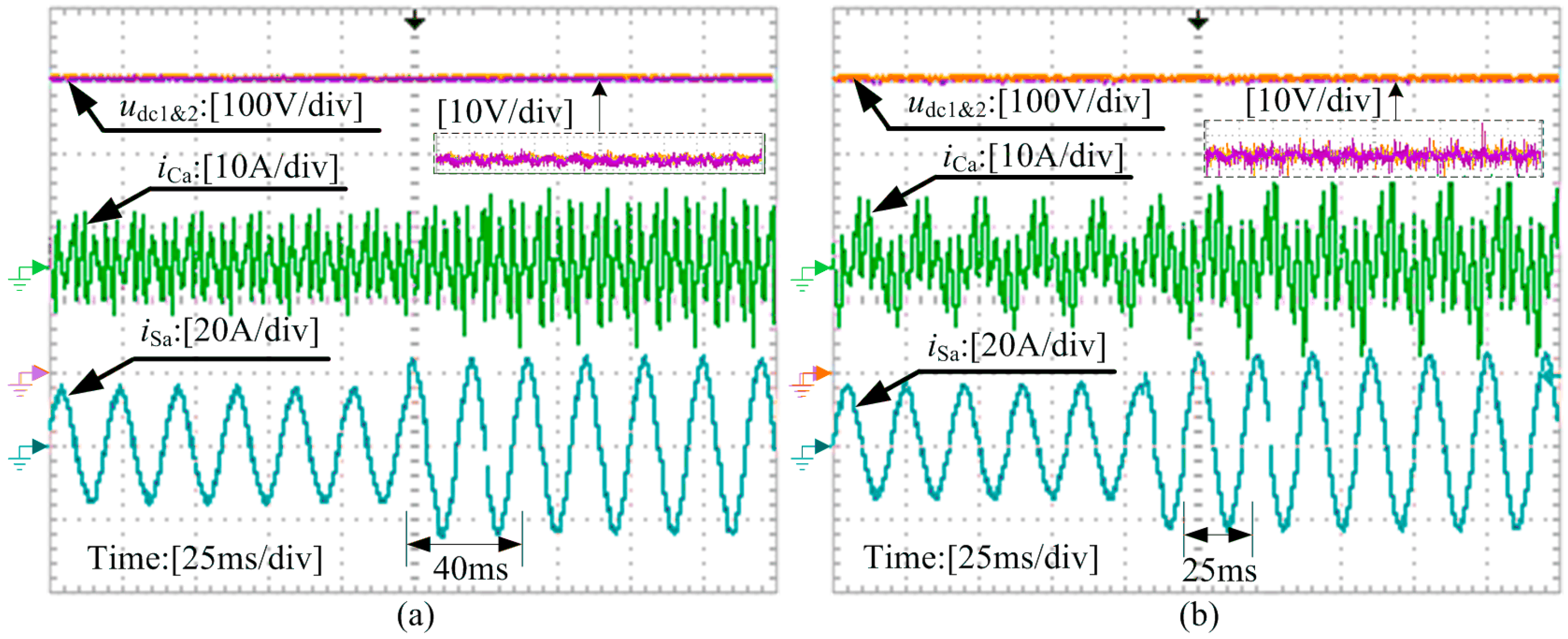
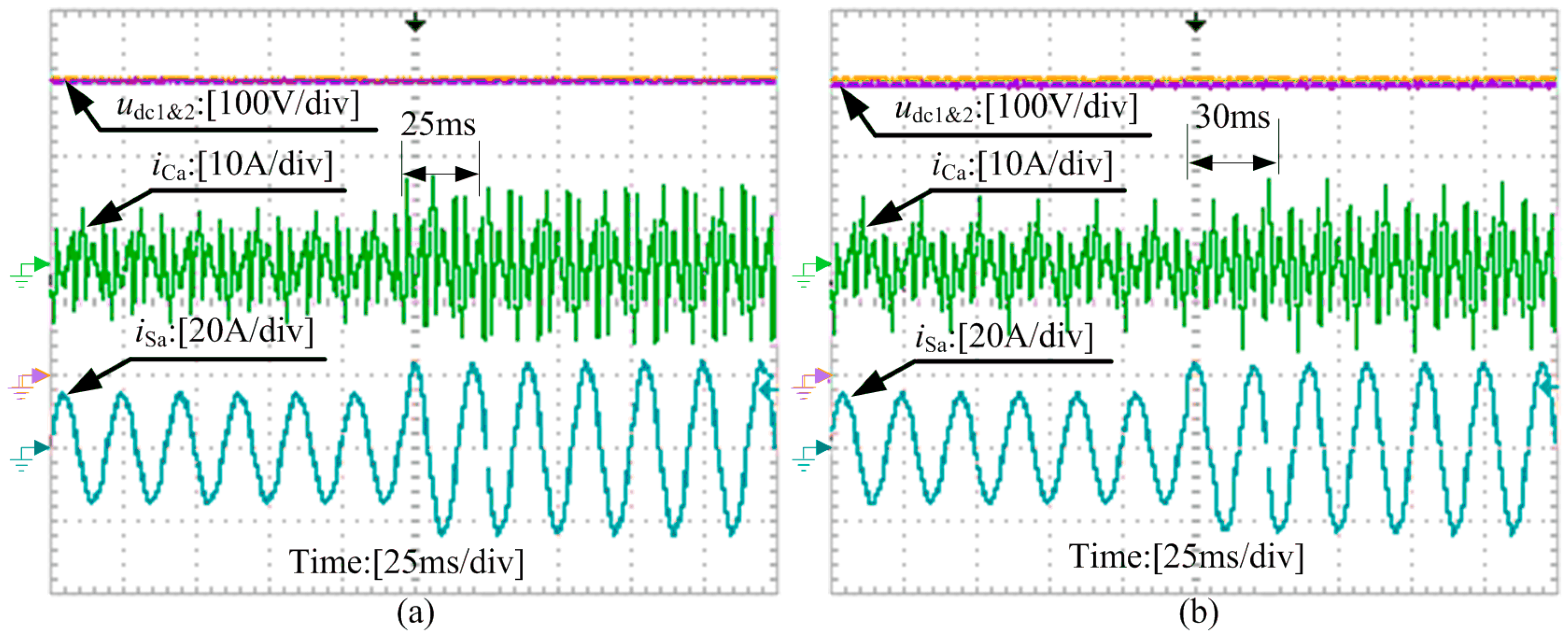
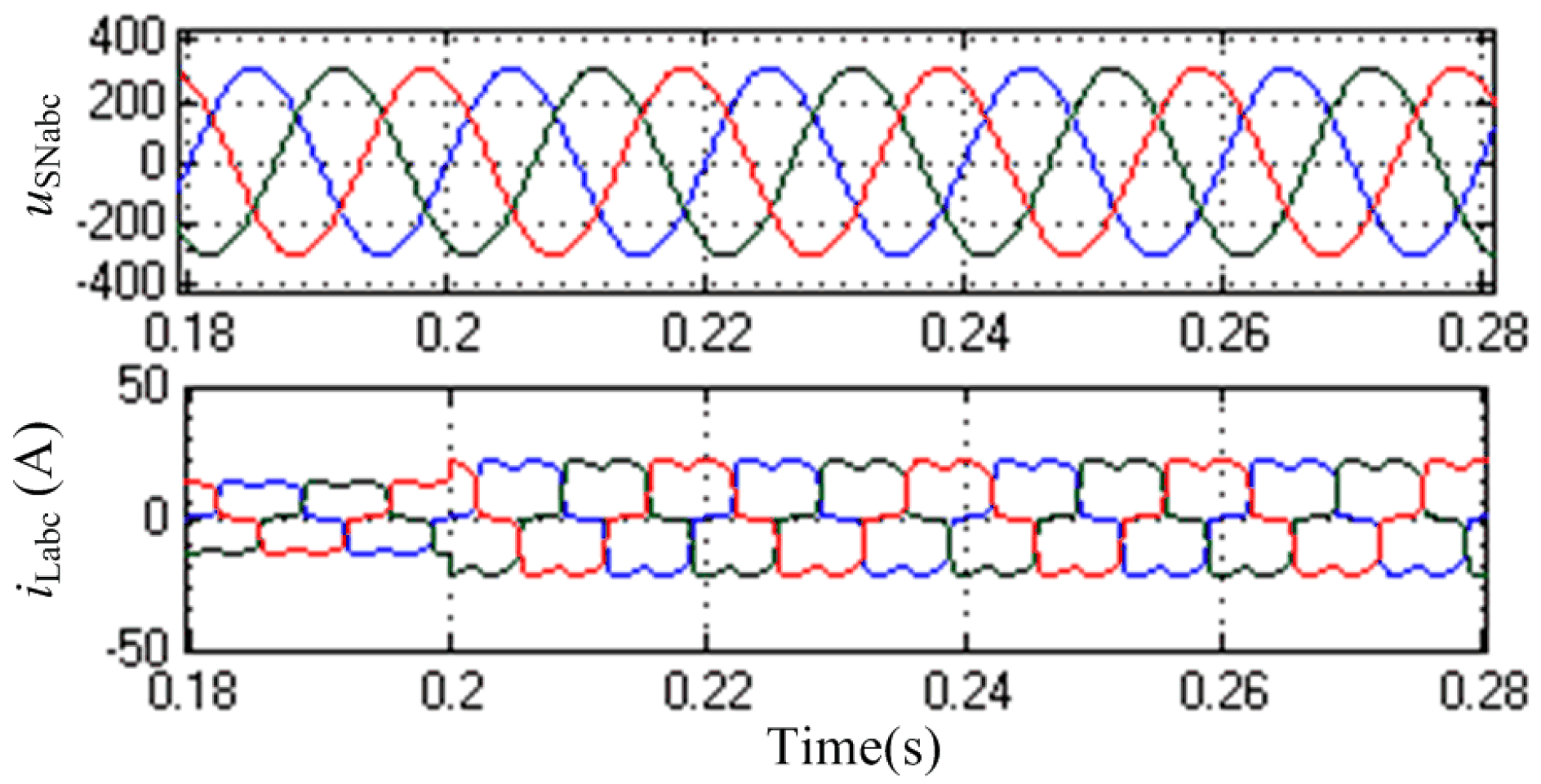
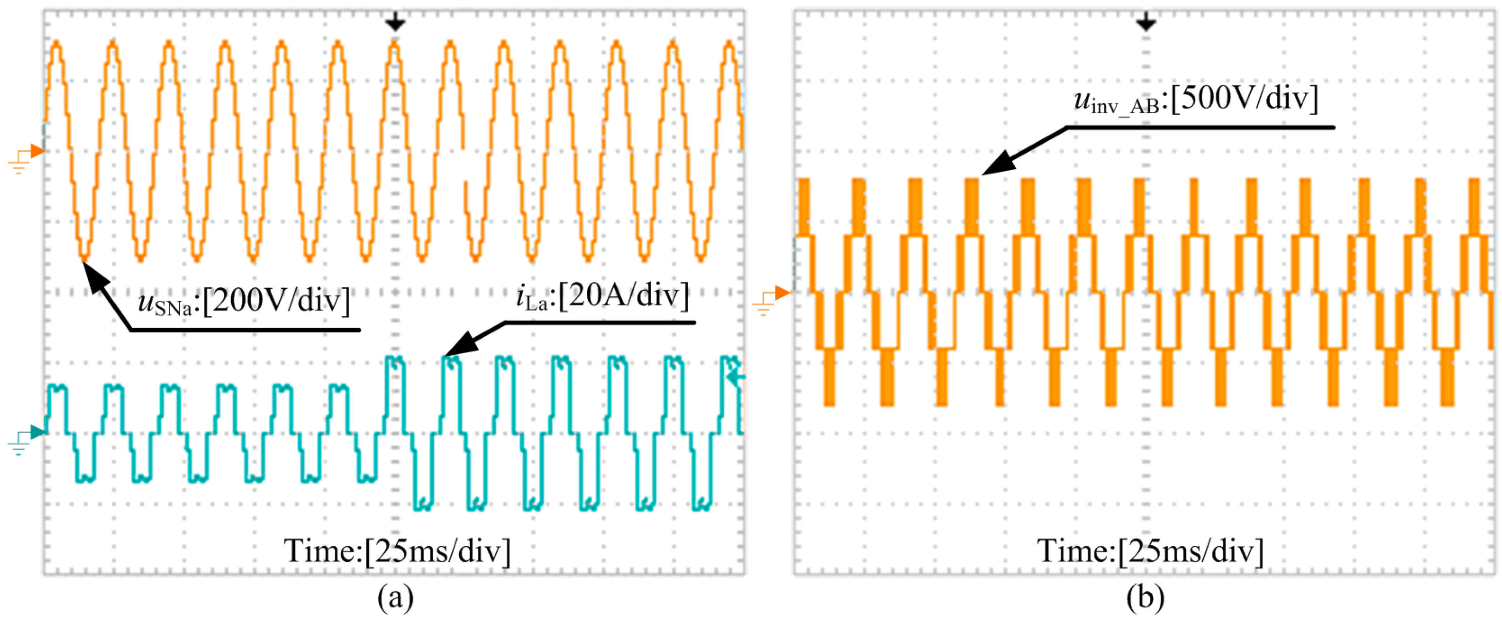
6.1. Dynamic Response of the NPC-SAPF

Phase A grid voltage (u_SNa), nonlinear load current (i_La) and output line-to-line voltage (u_{inv_AB}) of NPC are shown in Figure 14. This is the PCC voltage and load current condition of the rest experiments. There are three voltage levels of NPC-SAPF: 0, 400 and 800 V in Figure 14b. Output current on gird-side inductor (i_Ca), grid current (i_Sa) and upper and lower DC-capacitor voltages (u_dc1&2) are shown in Figure 15. The step-change of the nonlinear load is the same as the simulation condition.

As shown in Figure 15, the upper and lower DC-capacitor voltages are equal and the DC voltage waveforms are regulated at the reference value (800 V). The waveforms of i_Sa and u_dc1&2 when λ = −1 × 10⁻² are more smooth than λ = −1 × 10⁻³. While the settling time of λ = −1 × 10⁻² (40 ms) is longer than λ = −1 × 10⁻³ (25 ms). It can be figured out that the overshoots of i_Ca and u_dc are very small. The results confirm that the NPC-SAPF can achieve fast dynamic response with small overshoot for a step-change of the nonlinear load.

6.2. Steady-State Performance of the NPC-APF

The NPC-SAPF operates stably after 40 ms from the step-change point. The FFT analysis conducted by SIMULINK/powergui function of phase A grid currents are shown in Figure 16 and the detailed experimental data when λ = −1 × 10⁻² are shown in

Table 3. Detailed experimental data.

Harmonic Order	Load Current		Grid Current
	Amplitude (A)	Percent (%)	Amplitude (A)	Percent (%)
1	22.96	100	23.03	100
5	5.08	22.10	0.36	1.56
7	2.39	10.41	0.37	1.61
11	1.92	8.36	0.16	0.69
13	1.25	5.44	0.19	0.83
17	1.10	4.79	0.17	0.74
19	0.75	3.27	0.13	0.56
23	0.66	2.87	0.12	0.52
25	0.48	2.09	0.12	0.52
29	0.46	2.00	0.13	0.56
31	0.31	1.35	0.12	0.52
35	0.30	1.31	0.07	0.30
37	0.20	0.87	0.06	0.26
41	0.18	0.78	0.07	0.30
43	0.12	0.52	0.05	0.22
47	0.12	0.52	0.05	0.22
49	0.07	0.30	0.06	0.26
THD (%)	27.9		3.0

. The THD of the grid current is decreased from 27.9% (22.96 A fundamental) to 2.94% and 4.35% when λ = −1 × 10⁻² and λ = −1 × 10⁻³, respectively. In Table 3, we can figure out that each order harmonic percent is lower than IEEE Standard 519-2014 when λ = −1 × 10⁻². The experimental results conform with the simulation, and λ = −1 × 10⁻² is recommended. In addition, the switching frequency is not shown in Figure 16 because the number of data sample points provided by the Tektronix oscilloscope is not enough, but we can figure out that grid current waveforms in Figure 15 are very smooth, which indicates that the switching frequency harmonics are attenuated.

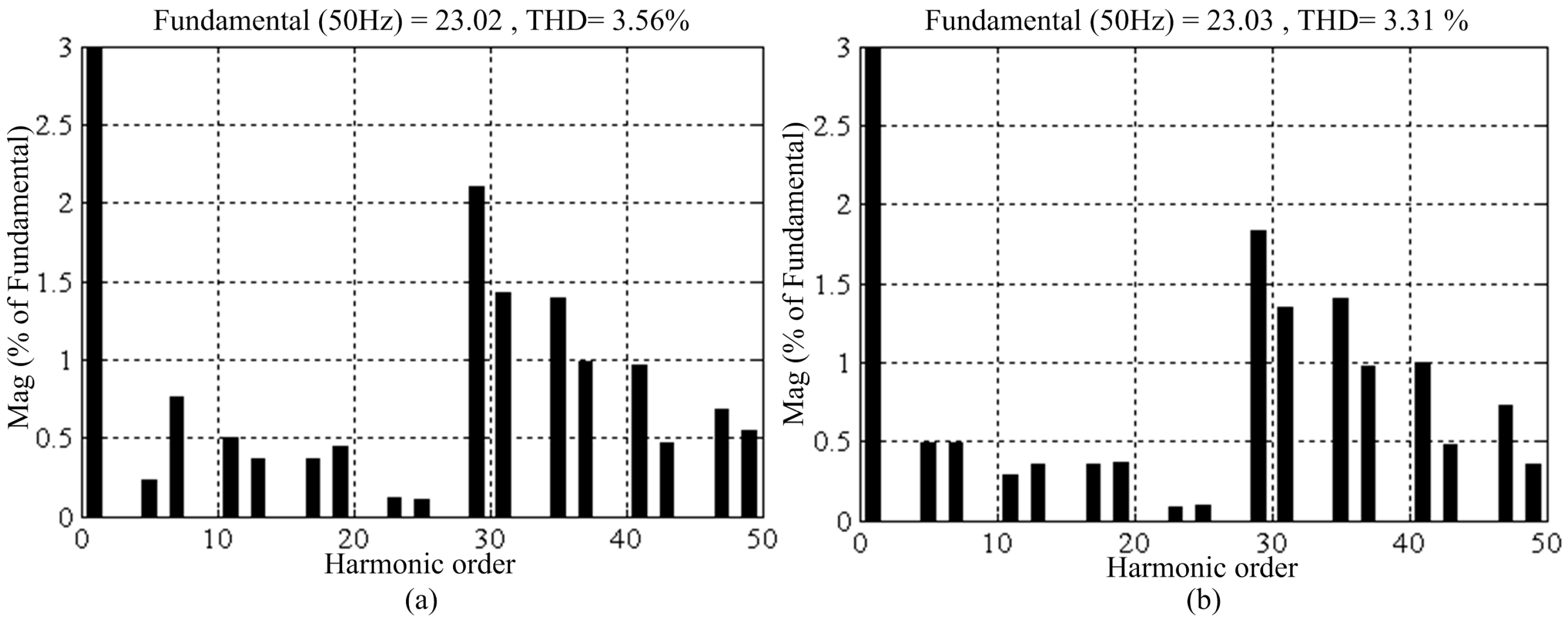
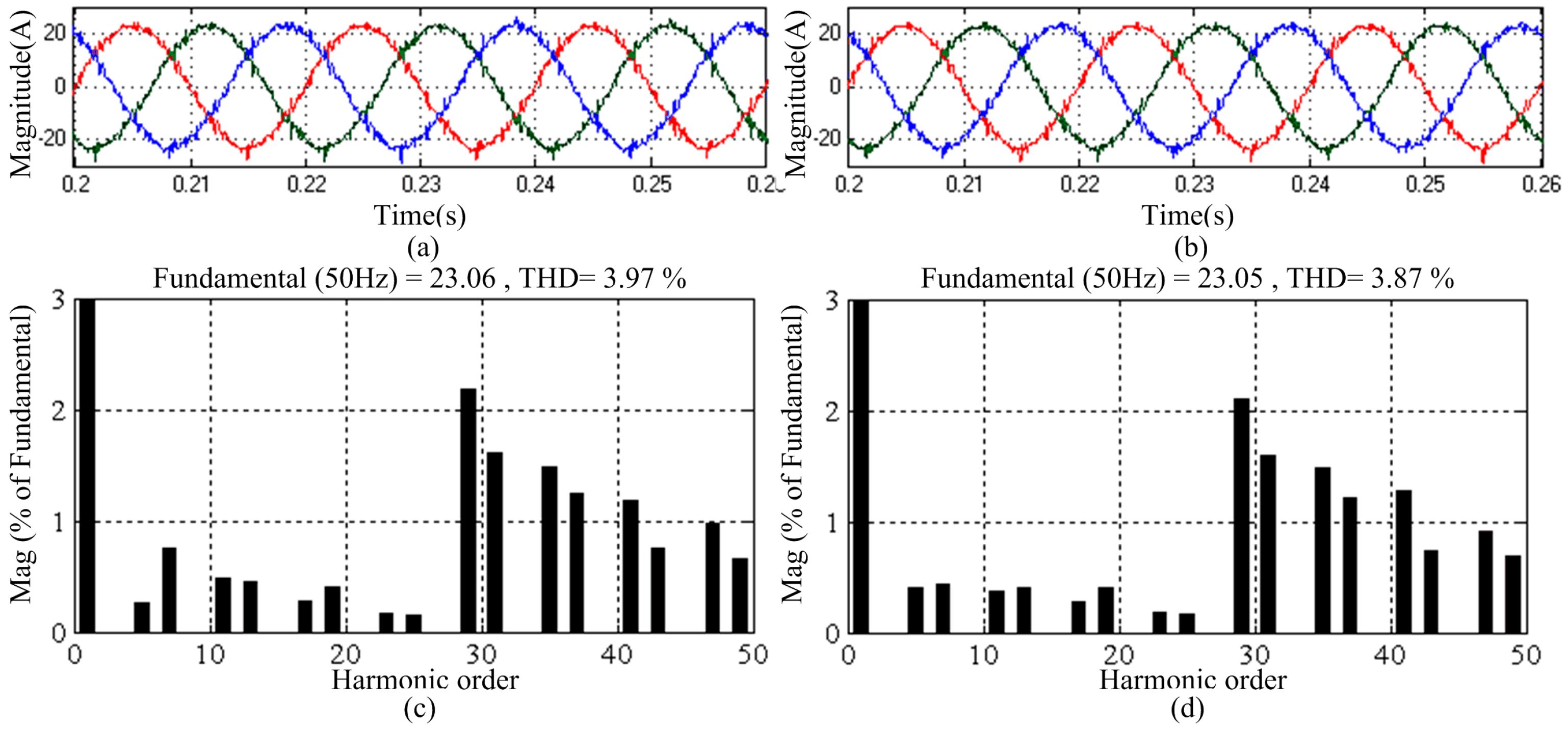
6.3. Experimental Resultes of PR and VPI Controllers

In order to clarify the advantages of the proposed control strategy with λ = −1 × 10⁻², the PR and VPI control methods in [3,13] were also applied in the NPC-SAPF prototype. According to the crossover frequency of the open-loop transfer function in Figure 4, the NPC-SAPF outputs 1st–25th harmonic currents. The experimental results are shown in Figure 17. The corresponding FFT analysis of phase A grid current is shown in Figure 18.

It can be seen from Figure 17 and Figure 18 that the THD grid currents in the two conditions are 4.07% and 4.01%. The 5th–25th harmonics are well attenuated while the 29th–50th harmonics still cannot meet the requirements of IEEE Standard 519-2014. The settling time of the output currents are only 25 ms and 30 ms, and the overshoot of output currents is very small.

In Section 6.2, the THD of grid current when λ = −1 × 10⁻² was 2.94%. The 5th–50th harmonics of the grid current are all attenuated and can satisfy the requirements of IEEE Standard 519-2014. In Section 6.1, the settling time of the output current was 40 ms, and the overshoot of the output current was also small when λ = −1 × 10⁻².

The THD of the proposed control strategy (3.0%) is superior to PR (3.56%) and VPI (3.31%) control methods. This is because the proposed control strategy compensates more high-frequency (29th–49th) harmonics than PR and VPI control methods. Besides, the settling time of the proposed control strategy is slightly poorer than PR and VPI control methods but it is acceptable.

From the above comparison results, we can conclude that the proposed control strategy has a satisfactory compensation performance without deteriorating the settling time severely compared with PR and VPI control methods.

7. Conclusions

In this paper, a Lyapunov stability theory-based control strategy for a three-phase three-wire NPC-SAPF is proposed and implemented to broaden the output bandwidth. By constructing the switching function on the basis of a mathematical model and the Lyapunov candidate function, the proposed control law avoids introducing closed-loop feedback control and keeps the system globally asymptotically stable. The NP voltage balance approach and an improved LLCL filter are introduced to ensure the normal operation of NPC-SAPF. The comparison simulations and experimental results between the proposed strategy and the classical methods validated the effectiveness of the proposed control strategy. The results have demonstrated that the system is able to compensate harmonic currents from 1st to 50th without deteriorating the settling time severely, and ensure that each harmonic component of the grid currents meets the requirements specified in the IEEE Standard 519-2014.

References

1. Soeiro, T.B.; Kolar, J.W. Analysis of high-efficiency three-phase two- and three-level unidirectional hybrid rectifiers. IEEE Trans. Ind. Electron. 2013, 60, 3589–3601. [Google Scholar] [CrossRef]
2. Li, Z.; Li, Y.; Wang, P.; Zhu, H.; Liu, C.; Xu, W. Control of three-phase boost-type PWM rectifier in stationary frame under unbalanced input voltage. IEEE Trans. Power. Electron. 2010, 25, 2521–2530. [Google Scholar] [CrossRef]
3. Alejandro, G.Y.; Francisco, D.F.; Jesús, D.G.; Óscar, L. Effects of discretization methods on the performance of resonant controllers. IEEE Trans. Power. Electron. 2010, 25, 1692–1712. [Google Scholar]
4. Yi, T.; Poh, C.L.; Peng, W.; Fook, C.H. Generalized design of high performance shunt active power filter with output LCL filter. IEEE Trans. Ind. Electron. 2012, 59, 1443–1452. [Google Scholar]
5. Marcos, B.K.; Cursino, B.J. Virtual flux sensorless control for shunt active power filters with Quasi-resonant compensators. IEEE Trans. Power. Electron. 2016, 31, 4818–4830. [Google Scholar]
6. Bojoi, R.I.; Griva, G.; Bostan, V.; Guerriero, M. Current control strategy for power conditioners using sinusoidal signal integrators in synchronous reference frame. IEEE Trans. Power. Electron. 2005, 20, 1402–1412. [Google Scholar] [CrossRef]
7. Sun, J.J.; Gong, J.W.; Chen, B.F.; Zha, X.M. Analysis and design of repetitive controller based on regeneration spectrum and sensitivity function in active power filter system. IET Power. Electron. 2014, 7, 2133–2140. [Google Scholar] [CrossRef]
8. Aurelio, G.C.; Omar, P.A.; Vicente, F.B.; Pedro, R.S. Application of a repetitive controller for a three-phase active power filter. IEEE Trans. Power. Electron. 2007, 22, 237–246. [Google Scholar]
9. Zou, Z.X.; Wang, Z.; Cheng, M. Modeling, Analysis, and design of multifunction grid-interfaced inverters with output LCL filter. IEEE Trans. Power. Electron. 2014, 29, 3830–3839. [Google Scholar] [CrossRef]
10. Suresh, Y.; Panda, A.K.; Suresh, M. Real-time implementation of adaptive fuzzy hysteresis-band current control technique for shunt active power filter. IET Power. Electron. 2012, 5, 1188–1195. [Google Scholar] [CrossRef]
11. Chen, B.S.; Joós, G. Direct power control of active filters with averaged switching frequency regulation. IEEE Trans. Power. Electron. 2008, 23, 2729–2737. [Google Scholar] [CrossRef]
12. Wang, L.; Lam, C.S.; Wong, M.C.; Dai, N.Y. Non-linear adaptive hysteresis band pulse-width modulation control for hybrid active power filters to reduce switching loss. IET Power. Electron. 2012, 8, 2156–2167. [Google Scholar] [CrossRef]
13. Lascu, C.; Asiminoaei, L.; Boldea, I.; Blaabjerg, F. High performance current controller for selective harmonic compensation in active power filters. IEEE Trans. Power. Electron. 2007, 22, 1826–1835. [Google Scholar] [CrossRef]
14. Li, Y.; Liu, Q.Y.; Hu, S.J.; Liu, F.; Cao, Y.J.; Luo, L.F.; Rehtanz, C. A virtual impedance comprehensive control strategy for the controllably inductive power filtering system. IEEE Trans. Power. Electron. 2017, 32, 920–926. [Google Scholar] [CrossRef]
15. Li, Y.; Peng, Y.J.; Liu, F.; Sidorov, D.; Panasetsky, D.; Liang, C.G.; Luo, L.F.; Cao, Y.J. A controllably inductive filtering method with transformer-integrated linear reactor for power quality improvement of shipboard power system. IEEE Trans. Power Deliv. 2016, PP. [Google Scholar] [CrossRef]
16. Yuan, X.; Merk, W.; Stemmler, H.; Allmeling, J. Stationary-frame generalized integrators for current control of active power filters with zero steady-state error for current harmonics of concern under unbalanced and distorted operating conditions. IEEE Trans. Ind. Appl. 2002, 38, 523–532. [Google Scholar] [CrossRef]
17. IEEE Recommended Practice and Requirements for Harmonic Control in Electrical Power Systems; IEEE Standard 519-2014; IEEE: New York, NY, USA, 2014.
18. Komurcugil, H.; Altin, N.; Ozdemir, S.; Sefa, I. An extended Lyapunov-function-based control strategy for single-phase UPS inverters. IEEE Trans. Power. Electron. 2015, 30, 3976–3983. [Google Scholar] [CrossRef]
19. Kato, T.; Inoue, K.; Ueda, M. Lyapunov-based digital control of a grid-connected inverter with an LCL filter. IEEE J. Emerg. Sel. Top. Power Electron. 2014, 2, 942–948. [Google Scholar] [CrossRef]
20. Rahmani, S.; Hamadi, A.; Al-Haddad, K. A Lyapunov-function-based control for a three-phase shunt hybrid active filter. IEEE Trans. Ind. Electron. 2012, 59, 1418–1429. [Google Scholar] [CrossRef]
21. Meza, C.; Biel, D.; Jeltsema, D.; Scherpen, J.M.A. Lyapunov-based control scheme for single-phase grid-connected PV central inverters. IEEE Trans. Control Syst. Technol. 2012, 20, 520–529. [Google Scholar] [CrossRef]
22. Komurcugil, H.; Altin, N.; Ozdemir, S. Lyapunov-function and proportional-resonant-based control strategy for single-phase grid-connected VSI with LCL filter. IEEE Trans. Ind. Electron. 2016, 63, 2838–2849. [Google Scholar] [CrossRef]
23. Kwak, S.; Yoo, S.J.; Park, J. Finite control set predictive control based on Lyapunov function for three-phase voltage source inverters. IET Power. Electron. 2014, 7, 2726–2732. [Google Scholar] [CrossRef]
24. Dasgupta, S.; Mohan, S.N.; Sahoo, S.K. Lyapunov function-based current controller to control active and reactive power flow from a renewable energy source to a generalized three-phase microgrid system. IEEE Trans. Ind. Electron. 2013, 60, 799–813. [Google Scholar] [CrossRef]
25. Pou, J.; Zaragoza, J.; Ceballos, S.; Saeedifard, M. A carrier-based PWM strategy with zero sequence voltage injection for a three-level neutral-point-clamped converter. IEEE Trans. Power. Electron. 2012, 27, 642–651. [Google Scholar] [CrossRef]
26. Zaragoza, J.; Pou, J.; Ceballos, S. Voltage-Balance compensator for a carrier-based modulation in the neutral-point-clamped converter. IEEE Trans. Ind. Electron. 2009, 56, 305–314. [Google Scholar] [CrossRef]
27. López, I.; Ceballos, S.; Pou, J.; Saeedifard, M. Modulation strategy for multiphase neutral-point-clamped converters. IEEE Trans. Power. Electron. 2016, 31, 928–941. [Google Scholar] [CrossRef]
28. Wu, W.M.; He, Y.B.; Blaabjerg, F. An LLCL power filter for single-phase grid-tied inverter. IEEE Trans. Power. Electron. 2012, 27, 782–789. [Google Scholar] [CrossRef]
29. Wu, W.M.; He, Y.B.; Tang, T.H.; Blaabjerg, F. A new design method for the passive damped LCL and LLCL filter-based single-phase grid-tied inverter. IEEE Trans. Ind. Electron. 2013, 60, 4339–4350. [Google Scholar] [CrossRef]
30. Huang, M.; Wang, X.F.; Loh, P.C. Active damping of LLCL-filter resonance based on LC-trap voltage or current feedback. IEEE Trans. Power. Electron. 2016, 31, 2337–2346. [Google Scholar] [CrossRef]
31. Wu, W.M.; Sun, Y.J.; Huang, M. A robust passive damping method for LLCL-filter-based grid-tied inverters to minimize the effect of grid harmonic voltages. IEEE Trans. Power. Electron. 2014, 29, 3279–3289. [Google Scholar] [CrossRef]
32. Kömürcügil, H.; Kükrer, Ö. A new control strategy for single-phase shunt active power filters using a Lyapunov function. IEEE Trans. Ind. Electron. 2006, 53, 305–312. [Google Scholar] [CrossRef]
Figure 1. Configuration of the neutral-point-clamped shunt active power filter (NPC-SAPF) system.
Energies 10 00112 g001
Figure 2. Block diagram of the proposed control strategy. PCC: point of common coupling; PLL: phase lock loop; CB-PWM: carrier based pulse width modulation; and DFT: discrete Fourier transformation.
Energies 10 00112 g002
Figure 3. LLCL filter and the Bode plots. (a) Single structure of LLCL filter; and (b) bode plots of ig(s)/uf(s).
Energies 10 00112 g003
Figure 4. Current control model and open-loop Bode plots. (a) Current control model; and (b) open-loop Bode plots.
Energies 10 00112 g004
Figure 5. The three-dimensional plot of f(s, λ).
Energies 10 00112 g005
Figure 6. The relationship between α1 and g1max.
Energies 10 00112 g006
Figure 7. Output current of phase A on Lg and the fast Fourier transform (FFT) analysis. (a) Output current waveform by using the proposed control strategy; (b) output current waveform by using PR controllers; (c) output current waveform by using VPI controllers; (d) FFT analysis of current in (a); (e) FFT analysis of current in (b); and (f) FFT analysis of current in (c).
Energies 10 00112 g007
Figure 8. Grid current of phase A and the FFT analysis. (a) Grid current waveform by using PR controllers; (b) grid current waveform by using VPI controllers; (c) FFT analysis of current in (a); and (d) FFT analysis of current in (b).
Energies 10 00112 g008
Figure 9. Grid voltages and nonlinear load currents with step change.
Energies 10 00112 g009
Figure 10. Dynamic response of NPC-SAPF when λ = −1 × 10⁻².
Energies 10 00112 g010
Figure 11. Dynamic response of NPC-SAPF when λ = −1 × 10³.
Energies 10 00112 g011
Figure 12. The FFT analysis of phase A grid current in steady-state condition.
Energies 10 00112 g012
Figure 13. The 6.6 kVA NPC-SAPF system.
Energies 10 00112 g013
Figure 14. Experimental conditions of phase A. (a) Grid voltage and nonlinear load current; and (b) output line-to-line voltage of NPC.
Energies 10 00112 g014
Figure 15. Dynamic response of NPC-SAPF. (a) λ = −1 × 10⁻²; and (b) λ = −1 × 10³.
Energies 10 00112 g015
Figure 16. The FFT analysis of grid currents in steady-state condition.
Energies 10 00112 g016
Figure 17. Dynamic response of NPC-SAPF by using PR and VPI control methods. (a) PR control method; and (b) VPI control method.
Energies 10 00112 g017
Figure 18. The FFT analysis of grid currents in steady-state condition. (a) PR control method; and (b) VPI control method.
Energies 10 00112 g018