Development of a Numerical Weather Analysis Tool for Assessing the Precooling Potential at Any Location

Abstract

Precooling a building overnight during the summer is a low cost practice that may provide significant help in decreasing energy demand and shaving peak loads in buildings. The effectiveness of precooling depends on the weather patterns at the location, however research in this field is predominantly focused in the building thermal response alone. This paper proposes an analytical tool for assessing the precooling potential through simulations from real data in a numerical weather prediction platform. Three dimensionless ratios are developed based on the meteorological analysis and the concept of degree hours that provide an understanding of the precooling potential, utilization and theoretical value. Simulations were carried out for five sites within the Sydney (Australia) metro area and it was found that they have different responses to precooling, depending on their proximity to the ocean, vegetation coverage, and urban density. These effects cannot be detected when typical meteorological year data or data from weather stations at a distance from the building were used. Results from simulations in other Australian capitals suggest that buildings in continental and temperate climates have the potential to cover substantial parts of the cooling loads with precooling, assuming appropriate infrastructure is in place.

1. Introduction

Passive energy management is of particular interest to building energy system research, as clever design or operation policies may result in significant financial or energy savings at little or no additional cost. The optimisation of energy performance of large commercial buildings is associated with managing heating, ventilation and air-conditioning (HVAC) loads, as in most cases they are responsible for the highest overall energy consumption [1,2,3], as well as major peaks of the total load [3,4,5]. Examples of passive measures include the optimisation of orientation of the building related to the sun’s path, the utilisation of natural lighting or ventilation, using the thermal mass of the building to discharge energy with a phase lag, and the preconditioning of buildings. Preconditioning describes a set of measures that make it possible to shift parts of the heating or cooling load to different time periods in order to save on energy costs and if done without any energy expenditure to reduce total consumption as well. Precooling a building during the summer the night before using natural ventilation is an example of a common preconditioning practice [6].

The uncertainty linked to weather predictions that affect preconditioning, is mainly realised as a modelling problem. An additional component of uncertainty is that local weather conditions may vary notably even for sites separated by a few kilometres and hence generation of onsite forecasts is very relevant to energy performance optimisation. In this paper, an analytical tool is proposed that aims to help with assessing the potential of precooling at a specific site, based on historical weather data. Knowing this information can assist both designers of new buildings to add features that take advantage of high precooling potentials if available, as well as building managers seeking to upgrade existing energy management systems in order to improve the building performance.

The work presented in this paper constitutes part of a bundle of applications of numerical weather predictions and analyses in building energy management. The work is based on a numerical weather prediction and analysis software, called The Air Pollution Model (TAPM). TAPM’s meteorological tools have the capacity to provide accurate weather analyses and can be applied at any location, addressing both uncertainties explained above [7]. While TAPM was developed to model pollution flows in larger scales, its parameterisation allows its use for meteorological studies with high resolution.

Table 1. Terminology used in reference to TAPM simulations.

Term	Description
Domain	The domain is a 3-D space of custom dimensions in the shape of a rectangular prism. TAPM simulations and predictions occur within a particular domain.
Domain order	Higher order domains refer to domains of greater size, while lower order domains refer to domains of smaller size. Domains in TAPM exist within each other in successively lower orders.
Grid points	Each domain is divided in discrete grid points in all dimensions (x,y,z). Physical features, such as latitude, longitude, and elevation or vegetation index are stored in TAPM’s database for every grid point. Simulation results can be obtained at any grid point of any domain (but not at any other point of the domain).
Grid resolution	Grid points within the same domain are separated by a custom constant distance, which can be defined as the resolution. The resolution can be the same or different for each dimension.
Nesting ratio	The nesting ratio is defined as the ratio of the total areas on the ground level (x and y dimensions) of two consecutive order domains.

shows a list of the terminology used in this section, as well as throughout the following chapters when TAPM is involved.

The principles of operation of the meteorological component of TAPM involve solving fundamental equations of atmospheric dynamics in domains of gradually decreasing dimensions nested within each other, to calculate the evolution of weather variables [8,9]. The highest domain uses synoptic data as input, which are readily available and easily imported from sources such as the National Centre for Environmental Prediction (NCEP). The nesting ratios, number, resolution and size of each domain are user-defined. TAPM is capable of modelling the urban dynamic effects that affect the precooling potential, such as the vegetation coverage, landscape and sea breezes [10,11]. Furthermore, TAPM simulations can be run with rather low computational and time requirements.

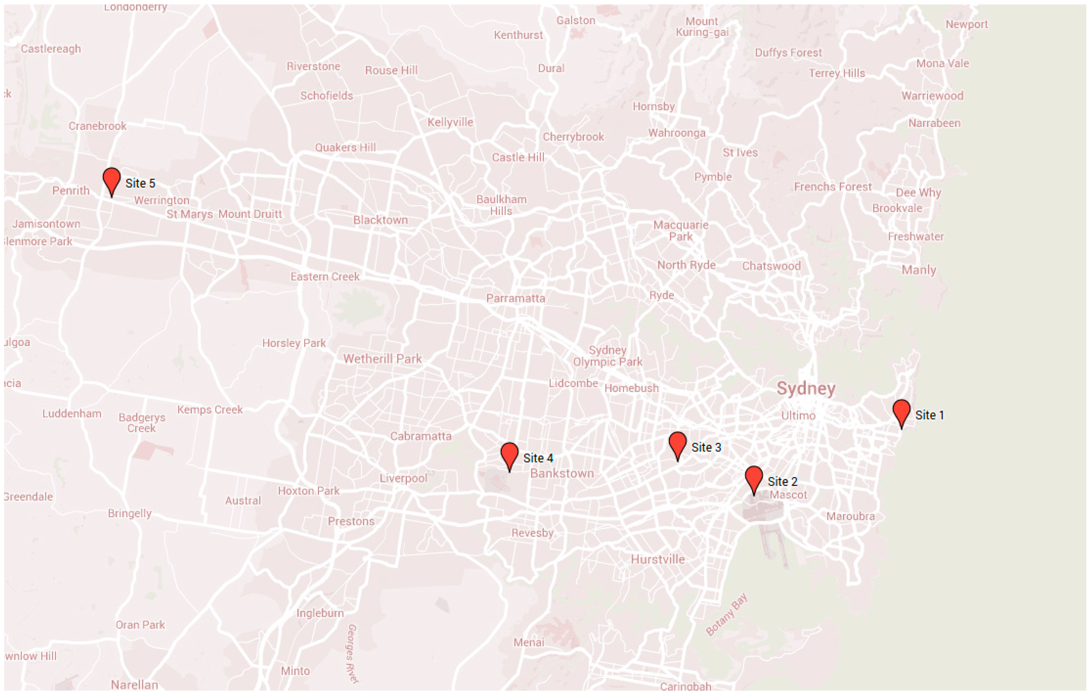
The proposed model is validated with the analysis of 7 years’ worth of data across five sites in the Sydney metropolitan area, in New South Wales, Australia, and other Australian capitals located in different climate zones. The assessment of the precooling potential is derived from the local climatic conditions and is independent of the building characteristics.

In addition to its applications in Building Energy Management Systems (BEMS) analytics, the tool attempts to extract some findings about the effects of a range of factors in regards to precooling potential. Specifically, the primary factor is expected to be the magnitude of diurnal temperature differences in the summer. Additionally, factors such as the proximity to large bodies of water, urban density and vegetation are considered in the analysis. The results indicate that the precooling potential varies for different areas according to the above factors and non-trivial savings may be achieved with appropriate designs.

Before describing the tool design methodology and simulation results, it is deemed necessary to discuss the existing literature on the field of preconditioning, as well as highlight the main features justifying the use of TAPM for the simulations.

Preconditioning refers to the process of adjusting the internal building conditions in advance, so that during the following time periods there is reduced energy consumption by the HVAC system and hence lower costs [6]. Temperature predictions of appropriate horizons are always required to assess the preconditioning potential savings and plan the control strategies. Depending on the building model, location and characteristics, savings up to 40% have been realised in many case study buildings around the world with preconditioning [12,13]. Preconditioning processes may be realised in various ways, but generally can be classified as either passive or active.

Passive preconditioning (ventilation via open windows, ducts, and utilisation of energy of the building’s thermal mass) takes advantage of the naturally occurring changes in the external conditions and the building design to condition the interior. The notion of taking advantage of diurnal temperature differences without significant energy expenditure, can result in “low cost” savings depending on the infrastructure in place. The opportunity for applying such measures has been demonstrated with studies that indicate night ventilation results in annual electrical cost reductions of up to 17% [14,15]. In addition to energy consumption reductions, in some instances passive preconditioning allows the replacement of the building air mass with fresher air from outside, improving the occupancy comfort [16]. Another advantage is that there is a net energy demand decrease, compared to active methods where the total energy required to “shift” some of the load to prior time zones is higher than the energy saved [17].

Active preconditioning with the HVAC system operating fully or partially, uses cheaper off-peak energy in advance to minimise peak energy demand during the day. Generally, these strategies are more reliable and consistent than passive ones as they can be applied regardless of the external temperature differences and can generate more significant peak load reductions. The peak load shaving is achieved by using the HVAC system overnight to precondition the building and hence reduce the energy needed for conditioning the day after [18]. In some cases the peak shaving is so effective (up to 75% reduction) that these strategies may be a viable alternative to upgrading components of the HVAC [19]. Nevertheless, the external weather conditions impact the cost of the implementation and hence weather forecasting is necessary for optimisation [19]. Lee and Braun [20] studied two active preconditioning strategies and compared them to the typical deterministic night setup. It was found that while the daily load overall is not significantly affected, the peak load is reduced thus leading to cost savings without compromising the comfort of the occupants. The effectiveness of this type of strategy assumes that weather and electricity inputs are considered in energy control [21].

Preconditioning planning involves the prediction of the internal temperature of a building zone as a function of the ambient temperature and the building features. The internal temperature must remain within certain comfort boundaries throughout the occupied period. Depending on the construction, the thermal mass of the building may significantly alter the effects of ambient weather on the indoor conditions. Envelopes constructed from heavy materials not only attenuate the changes in ambient temperature, but also add a notable temporal delay to the changes that follow in internal conditions of temperature, which is taken into account during preconditioning planning. On the contrary, lightweight constructions result in internal temperature ranges that are comparable to the ambient temperature and occur with very little lag [22].

It has been shown that due to the effects of the thermal mass of the building, small forecasting errors in ambient temperature (below 2–3 °C) tend to have relatively minor effects in optimisation of preconditioning and the thermal comfort (reductions of up to 20% reported) [23]. In essence, the indoor temperature display a lag—the magnitude of which depends on the building envelope—compared to the ambient temperature [24,25].

The literature also suggests that the long-term climate trends at the location of the building under question is a major factor for decision making in preconditioning strategies [14,26]. The variations in preconditioning effectiveness are easy to pinpoint when comparing sites across completely different climates [27]. Apart from the climate, geographical factors may affect the development of preconditioning policies. For instance, proximity to large masses of water typically diminishes diurnal differences in temperature due to the thermal mass of the ocean, and sea breezes. Hence passive preconditioning to cool down a building in the summer may not be possible. Other factors affecting local micro-climates and hence the preconditioning potential include vegetation coverage, landscape elevation, built environment density, type of urban zone and pollution [28,29]. Numerical modelling is particularly useful in such high spatial resolution analyses [30]. Of course the building characteristics are also vital when managing preconditioning strategies. Generally, heavy building envelopes result in superior peak load reductions than lighter construction buildings [31,32].

Most existing literature is concerned with the design of energy controllers and modelling the thermal response of the building to preconditioning rather than assessing the potential due to the local climate [33]. This work aims to address this research gap by developing a weather analysis tool to assist with development of preconditioning strategies.

2. Materials and Methods

2.1. Simulation Parameterisation

The proposed tool architecture is based on analysing downscaled synoptic data from past years at the location in question in order to develop a statistical analysis of the local climatic conditions. The database is then used to assess the precooling potential in the area.

Three nested domains were used in the simulations. Domain #1 has dimensions 40.5 km × 40.5 km, domain #2 has dimensions 13.5 km × 13.5 km and domain #3 has dimensions 4.5 km × 4.5 km. The resolution and number of domains were selected in order to minimise computational time without compromising forecasting accuracy. The selected configuration provides high accuracy at low simulation times and the ability to capture localised weather effects. The number of grid points in each domain for the model (x,y,z) was 25 × 25 × 25. The simulations were run at each site in hind-cast mode for seven years at five different locations. The primary output from the simulations consists of the ambient (dry bulb) temperature averaged for each hourly period of each year. The data processing to obtain meaningful findings for use within building energy optimisation was implemented via algorithms developed in Matlab.

2.2. Site Selection

The simulation sites belong to the Sydney metropolitan area and were selected to represent different weather locales. Figure 1 shows the locations of the sites, with the main factor during site selection being the proximity to the coast. Built environment density and vegetation were also considered.

The traits of each site are summarised in

Table 2. Characteristics of the five sites.

Site	Location	Distance to Coast	Urban Density	Vegetation
Site 1	Bondi	Coastal	High	Low
Site 2	Airport	1 km	Low	Low
Site 3	Canterbury	5 km	High	Low
Site 4	Bankstown	12 km	Moderate	Moderate
Site 5	Penrith	40 km	Low	Moderate

.

While the five sites are within a radius of about 35 km, the diurnal temperature differences vary and it is hypothesised that this will result in differences in evaluation of the precooling potential.

2.3. Precooling Conditions

In order for the tool to assess the potential for precooling, it needs to be configured to detect favourable conditions for the process to occur. For Sydney, during the summer months these conditions are met when:

• During the occupancy times (08.00–20.00) of a weekday, the ambient temperature rises above the upper boundary (25 °C)
• During the previous night (20.00–08.00), the ambient temperature falls below the lower boundary (20 °C)
• Relative humidity is maintained between 25% and 85%

These boundaries reflect typical Australian office indoor comfort conditions [34], adjusted for the effects of the thermal mass (attenuation, temporal lag) as described earlier in Section 1 and internal heat gains. Internal heat gains are highly variable and depend on the number of occupants, the occupant activity, operation of electronic and electrical devices, as well as the space layout [35]. It should be noted that the thermal comfort of an individual depends on various factors as well, such as the air temperature and relative humidity and are not constant throughout the year or even the course of a day. Other non-weather related factors include the ventilation rate, metabolism, clothing, and type of activity [36].

In such instances, energy can be saved by precooling the building the night before so that the cooling load of the daytime is reduced as discussed earlier. The precooling conditions were derived in relation to the comfort zone for each climate and the dampening of the changes in weather variables from outdoor to indoor environment. Additionally, the precooling conditions were established assuming light activity of occupants (representing typical commercial building occupant activity).

2.4. Precooling Ratios

The proposed methodology in this article, which may be used to assess the precooling potential and its theoretical value according to the ambient weather conditions, is based on a range of statistical ratios. The ratios are in turn based on the concept of degree-hours (DH). The DH are calculated as the amount of hours that the ambient temperature exceeds or is below a certain base temperature multiplied by the magnitude of the difference [37]. The base temperatures are set according to the precooling conditions described in Section 2.3. The advantage of modelling with DH compared to other regression or physical models is the relative simplicity and direct correlation of the building’s load to the weather conditions [38,39]. Three DH metrics were used in the development of the precooling ratios:

• DH_L: Represents the amount of degree-hours that the ambient temperature falls below the lower boundary (20 °C) during the night non-occupied period
• DH_U: Represents the amount of degree-hours that the ambient temperature rises above the upper boundary (25 °C) during the daytime occupied period
• DH_N: Represents the amount of degree-hours that the ambient temperature is below the upper boundary (25 °C) during the daytime occupied period

Additionally, the number of days that the precooling conditions are met in a single year (n) is used in the evaluation of the precooling ratios. An illustration of a daily profile showing the calculation of the DH values for a sample day can be seen in Figure 2.

For the sample day displayed in Figure 2, the DH_L is calculated as the sum of the differences of the ambient temperatures below the lower threshold (20 °C) at each time step during the vacant period (time steps 0 to 12).The DH_N and DH_U are calculated as the sums of differences of the ambient temperatures below and above the upper threshold (25 °C) respectively, at each time step during the occupied period (time steps 13 to 24).

Table 3. Calculation of the DH values for each time step for the sample day. The summation of the values in the end represents the values of DH_L, DH_N, and DH_U used in the precooling ratios.

Time Step	Ambient Temperature	DHL	DHN	DHU
1	21.4	0	N/A	N/A
2	20.1	0	N/A	N/A
3	19.1	0.9	N/A	N/A
4	18.5	1.5	N/A	N/A
5	17.9	2.1	N/A	N/A
6	17.5	2.5	N/A	N/A
7	17.1	2.9	N/A	N/A
8	17	3	N/A	N/A
9	16.9	3.1	N/A	N/A
10	16.8	3.2	N/A	N/A
11	16.9	3.1	N/A	N/A
12	18.4	1.6	N/A	N/A
13	20.8	N/A	4.2	0
14	23.1	N/A	1.9	0
15	25	N/A	0	0
16	26.6	N/A	0	1.6
17	27.8	N/A	0	2.8
18	28.7	N/A	0	3.7
19	29.2	N/A	0	4.2
20	29.3	N/A	0	4.3
21	29	N/A	0	4
22	28.5	N/A	0	3.5
23	27.1	N/A	0	2.1
24	25	N/A	0	0
Total	-	23.9	6.1	26.2

shows the actual calculations for each time step of the same sample day, in order to illustrate the methodology of deriving the DH values.

2.4.1. Precooling Potential

For the days when precooling conditions are met, the precooling potential ratio (r₁) can be defined as:

$${\mathrm{r}}_1=\frac{{{\displaystyle \sum }}_{\mathrm{i}=1}^{\mathrm{n}}\frac{{\mathrm{DH}}_{\mathrm{L}}\left(\mathrm{i}\right)}{{\mathrm{DH}}_{\mathrm{U}}\left(\mathrm{i}\right)}}{\mathrm{n}}$$

(1)

The potential for precooling would be higher for days preceded by cooler nights (temperature drops below 20 °C overnight and hence large value of DH_L) and followed by days with relatively low cooling loads during the occupied times (temperature rises only a few degrees above 25 °C and hence lower value of DH_U). During very hot days (high value of DH_U), the potential for precooling would be lower, as any overnight cooling would only be able to cover a minor part of the much larger cooling load during the daytime.

This is represented in the sum of fractions in the numerator for each hourly time step i. The ratio r₁ is averaged across all precooling days by dividing the sum by the number of days per year that the precooling conditions were met (n) (as calculated from the weather analysis of historical data).

If the potential ratio is close to 1, that means that the cooling overnight (DH_L) is just enough to cover the needs for cooling the day for the times that the temperature rises above 25 °C (DH_U). However, higher values of r₁, are not necessarily useful, as they may result from relatively cold summer days (which would have a low value of DH_U), during which the building cooling requirements are low anyway.

2.4.2. Precooling Utilisation

In addition to r₁ (potential ratio), it is possible to calculate the utilisation ratio r₂. This refers to the ratio of precooling degree-hours during the night before (DH_L) divided by the degree-hours that ambient temperature is below the upper boundary during the daytime (DH_N):

$${\mathrm{r}}_2=\frac{{{\displaystyle \sum }}_{\mathrm{i}=1}^{\mathrm{n}}\frac{{\mathrm{DH}}_{\mathrm{L}}\left(\mathrm{i}\right)}{{\mathrm{DH}}_{\mathrm{N}}\left(\mathrm{i}\right)}}{\mathrm{n}}$$

(2)

A higher utilisation ratio would indicate that most of the precooling was useful in mitigating cooling loads. This is because the denominator value (DH_N) would be small during hot days that temperature stays over 25 °C for most of the time. Hence any precooling overnight (proportional to DH_L) would contribute towards reducing the following day’s cooling loads.

If on the other hand, the utilisation ratio is small, it implies that the precooling occurring the night before (DH_L) was not making significant impact in reducing the day’s cooling load. This can be observed when the ambient temperature does not rise to high levels for long periods during the daytime (hence larger value of DH_N). During these days, the cooling load requirements would be comparatively lower to a hot summer day. As described earlier in Section 2.4.1, this may result in very high values (above 10–15) for r₁. This can also be observed when the temperature does not drop below 20 °C for long overnight (hence low value of DH_L). As with r₁, r₂ is averaged across all precooling days by dividing by n.

2.4.3. Precooling Frequency and Annualised Ratios

Another important ratio that can be derived from analysis of the historical weather data for the location is the precooling frequency (h), which is defined as the ratio of days that the precooling conditions are met (n) over the number of days in a year (365). The precooling frequency is used to annualise both the precooling and utilisation ratios. Annualising is necessary as the ratios by themselves convey information only about precooling days (when the conditions of Section 2.3 are met), and do not include any component of the frequency they occur throughout a year. Hence the annualised forms of both ratios (R) are calculated by multiplying each one with the precooling frequency ratio h:

$${\mathrm{R}}_1={\mathrm{r}}_1\mathrm{h}$$

(3)

$${\mathrm{R}}_2={\mathrm{r}}_2\mathrm{h}$$

(4)

The physical significance of Equations (3) and (4) is that they allow the comparison of climatological conditions on an annual basis, as opposed to the ratios r₁ and r₂, which can be used for comparisons only for the days that the precooling conditions are met. This is necessary, as for some sites the precooling potential may be high, but the precooling conditions are not met often, and hence the overall potential would not be significant throughout a year.

2.4.4. Theoretical Precooling Value

While both ratios r₁ and r₂ can assist in making useful conclusions about the precooling potential at a given site individually, there may be certain challenges in interpreting the theoretical precooling value. Hence, a value ratio can be calculated that incorporates dimensions of both the potential and utilisation of precooling. The theoretical value of precooling v(i) at a particular day i is calculated as the ratio of the difference of degree hours the temperature falls below the lower boundary the night before $({\mathrm{DH}}_{\mathrm{L}})$ minus the degree hours that the temperature does not rise above the upper boundary the day after $({\mathrm{DH}}_{\mathrm{N}})$ over the degree hours that the temperature rises above the upper boundary the day after $({\mathrm{DH}}_{\mathrm{U}})$:

$$\mathrm{v}\left(\mathrm{i}\right)=\frac{{\mathrm{DH}}_{\mathrm{L}}\left(\mathrm{i}\right)-{\mathrm{DH}}_{\mathrm{N}}\left(\mathrm{i}\right)}{{\mathrm{DH}}_{\mathrm{U}}\left(\mathrm{i}\right)}$$

(5)

A negative numerator indicates that DH_N is lower than DH_L for that day. In simple terms, this occurs when temperatures during most of the daytime are relatively cool (below 25 °C) making DH_N large. In addition, the temperatures during the night before remain relatively high, close to the lower boundary of 19 °C, making the value of DH_L small. The more negative the ratio v, the less value can be realised in precooling during these mild days. On the contrary, a positive numerator shows there is a significant diurnal temperature difference and that the precooling that occurs overnight can be utilised the day after to reduce the cooling load. The bigger the ratio, the more value can be realised.

Using Equations (1)–(5), the annualised value (V) can be rewritten as:

$$\mathrm{V}={\mathrm{R}}_1-\frac{{\mathrm{R}}_1}{{\mathrm{R}}_2}$$

(6)

It should be noted that Equation (6) shows the theoretical precooling value, based on the analysis of the historical weather trends. This can be regarded as the maximum value that may be extracted via the process of precooling, but in practice the actual value may be limited by the building’s characteristics and BEMS policies.

3. Results

3.1. Results Summary

The results of the simulations for the frequency, potential and utilisation ratios are summarised for all sites across Sydney in

Table 4. Summary of results across five sites in Sydney for each simulation year.

Site 1—Bondi	2014	2013	2012	2011	2010	2006	2005
h (frequency)	0.06	0.08	0.05	0.04	0.07	0.09	0.06
Precool days	21	28	19	16	26	34	22
r1 (potential)	24.8	41.0	7.9	22.6	17.6	10.3	10.4
R1	1.4	3.2	0.4	1.0	1.3	1.0	0.6
r2 (utilisation)	0.54	0.64	0.43	0.41	0.36	0.48	0.44
R2	0.03	0.05	0.02	0.02	0.03	0.04	0.03
Site 2—Airport	2014	2013	2012	2011	2010	2006	2005
h (frequency)	0.14	0.16	0.14	0.09	0.13	0.17	0.17
Precool days	52	57	51	34	48	63	60
r1 (potential)	23.5	8.8	14.1	10.0	14.4	5.8	9.1
R1	3.4	1.4	2.0	0.9	1.9	1.0	1.5
r2 (utilisation)	0.81	1.05	0.87	0.76	0.77	0.98	0.95
R2	0.12	0.17	0.12	0.07	0.10	0.17	0.16
Site 3—Canterbury	2014	2013	2012	2011	2010	2006	2005
h (frequency)	0.17	0.20	0.17	0.12	0.19	0.21	0.23
Precool days	60	72	61	43	70	76	84
r1 (potential)	19.0	9.8	18.6	2.8	13.7	9.7	25.0
R1	3.1	2.0	3.1	0.3	2.6	2.0	5.8
r2 (utilisation)	1.17	1.25	1.09	0.92	1	1.42	1.2
R2	0.19	0.25	0.18	0.11	0.19	0.3	0.28
Site 4—Bankstown	2014	2013	2012	2011	2010	2006	2005
h (frequency)	0.21	0.24	0.20	0.15	0.24	0.26	0.28
Precool days	78	88	73	54	87	94	101
r1 (potential)	11.0	19.7	14.7	6.7	16.5	7.7	9.1
R1	2.4	4.8	3.0	1.0	3.9	2	2.5
r2 (utilisation)	1.36	1.45	1.42	1.17	1.24	1.64	1.61
R2	0.29	0.35	0.28	0.17	0.3	0.42	0.45
Site 5—Penrith	2014	2013	2012	2011	2010	2006	2005
h (frequency)	0.21	0.22	0.18	0.13	0.19	0.21	0.28
Precool days	78	80	66	47	70	78	103
r1 (potential)	20.9	6.9	10.2	9.4	24.0	5.6	12.5
R1	4.5	1.5	1.9	1.2	4.6	1.2	3.5
r2 (utilisation)	1.76	1.87	1.74	1.3	1.35	2.01	2.01
R2	0.38	0.41	0.31	0.17	0.26	0.42	0.57

. It should be noted that synoptic data for the period 2007–2009 was not available and hence simulations for that period were omitted.

The results were compared to Typical Meteorological Year (TMY) Sydney data from the U.S. Department of Energy [40]. The data was developed for the Australia Greenhouse Office for use in complying with the Building Code of Australia and can be extracted in EnergyPlus. The comparison was carried out for the sake of investigating if the use of the proposed tool instead of using weather data in historical archives from external sources produces a more useful analysis. Specifically, the TMY data is provided for larger geographical areas, instead of being localised. Hence if the precooling potential and value differ across the sites, the TMY data will be less capable of showing the variations.

Table 5. Summary of precooling potential and utilisation across the five sites in Sydney.

Dataset	Site 1	Site 2	Site 3	Site 4	Site 5	TMY
h (frequency)	0.07	0.14	0.18	0.23	0.20	0.10
Average precooling occurrences	23.7	52.1	66.6	82.1	74.6	36.0
r1 (potential)	19.2	12.2	14.1	12.2	12.8	7.2
Annualised R1	1.3	1.7	2.7	2.8	2.6	0.7
r2 (utilisation)	0.47	0.88	1.15	1.41	1.72	0.54
Annualised R2	0.03	0.13	0.21	0.32	0.36	0.05

compares the final results over all years considered (2005–2006 and 2010–2014) for the ratios across all sites from the simulations and TMY data. The ratios in Table 4 are mean values averaged over the seven simulation years. The individual year results can be found in Table 3.

In the following sections, the results from the simulations for the five Sydney locations are going to be discussed in more detail.

3.2. Precooling Frequency

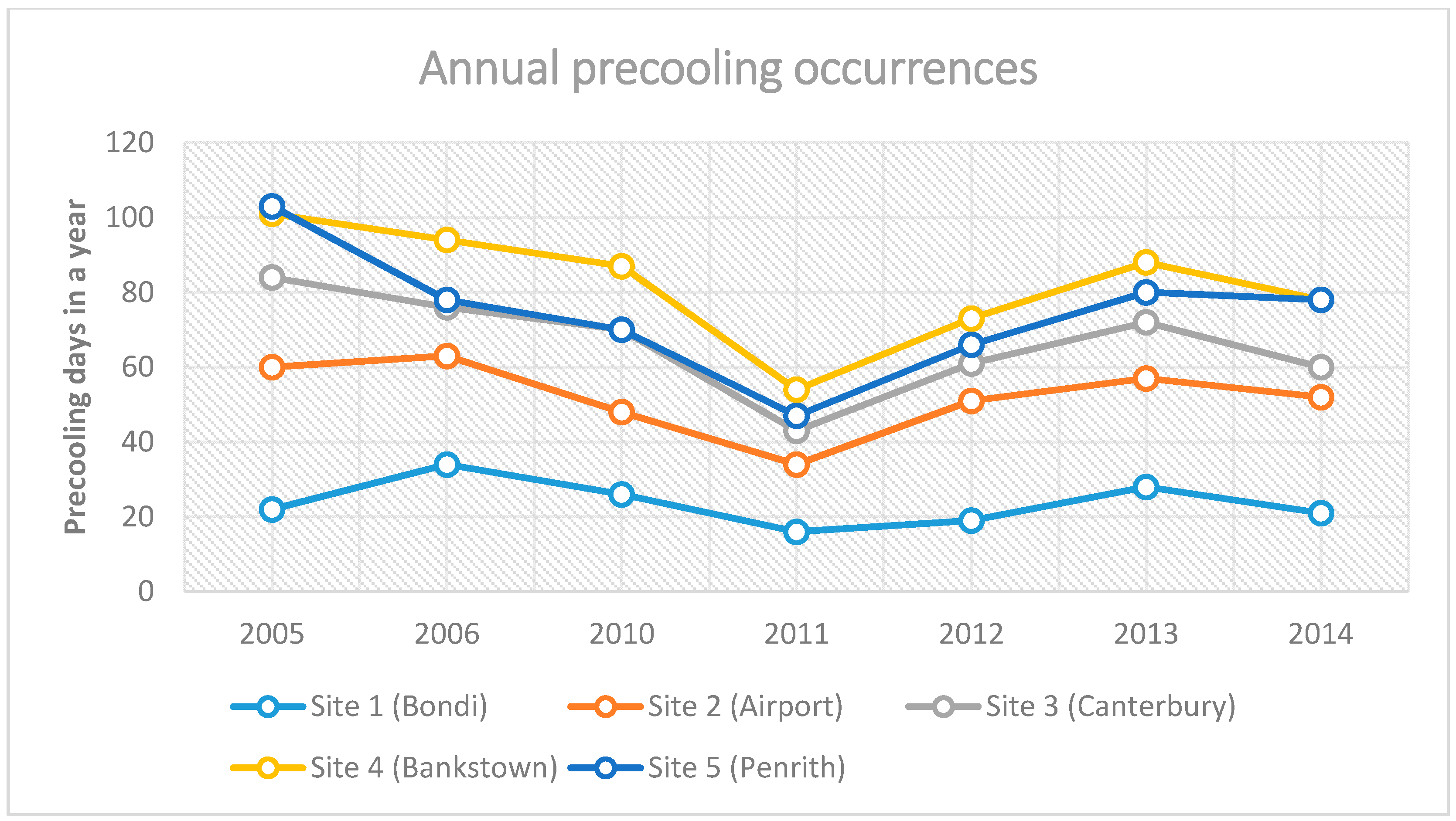
The occurrence of precooling days in a year and the frequency h were consistent throughout the simulation years, which is an indication that certain sites are more appropriate than others when implementing precooling measures. For example in 2011 the precooling frequency dropped notably for all sites, showing that during that summer, diurnal differences were lower than average. Figure 3 shows the gradients of the precooling occurrence curves, which display a similarity across all sites in Sydney. This was expected since the general climate over a year is similar for locations within a short range (of up to 50 km) of each other.

Sites 3, 4 and 5 (Bankstown, Canterbury and Penrith) had the highest frequency ratios, as they are further inland. For sites 1 and 2, the proximity to the ocean (enormous thermal mass) acts as a thermal buffer and tends to smooth the diurnal temperature differences, hence they occur less often.

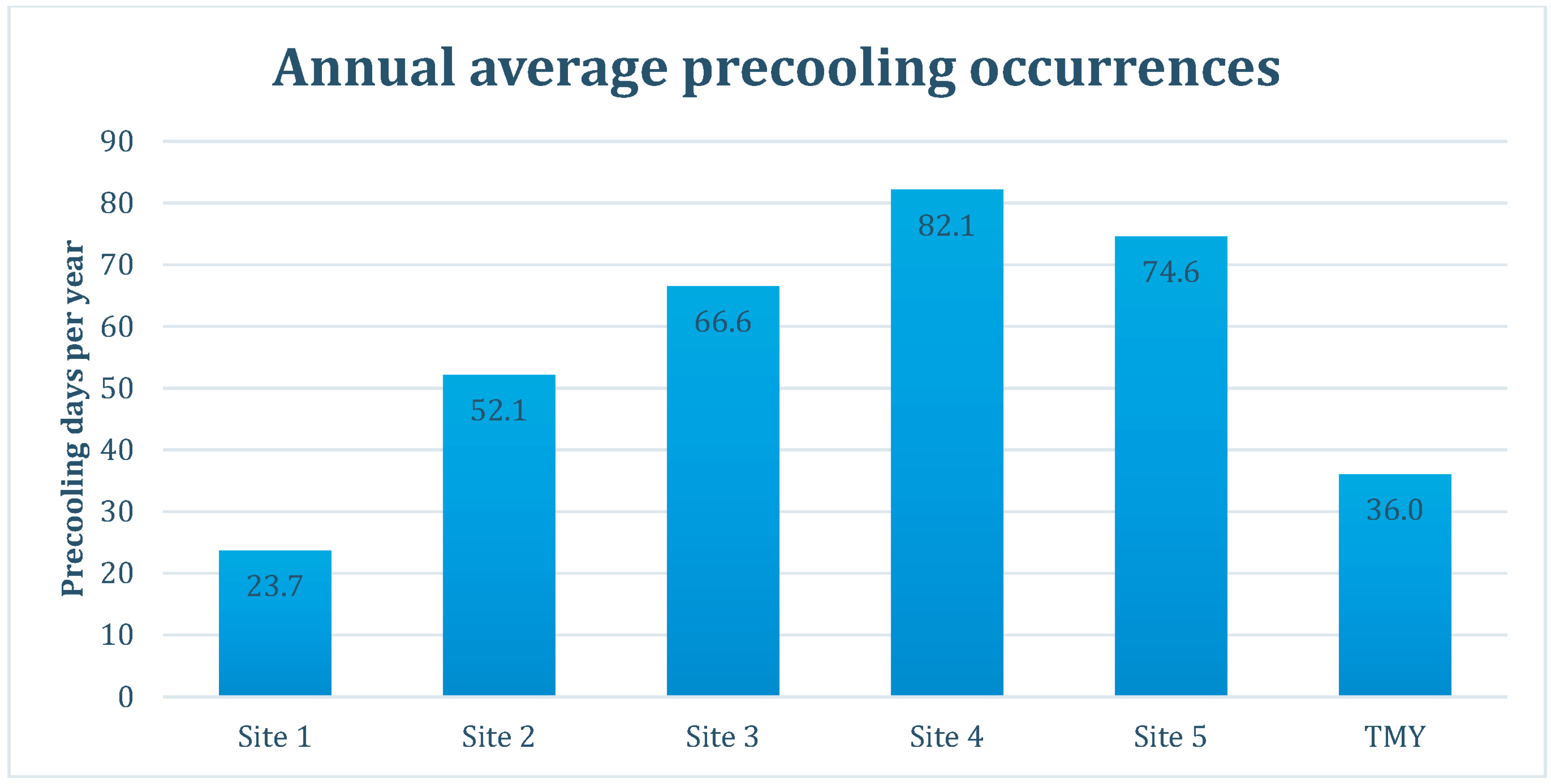
The average number of precooling days per year for each site and TMY data can be seen in Figure 4. The TMY data for frequency showed a flat rate of 36 precooling days across the metro Sydney area, however, as seen from the analysis based on the numerical simulations from real data, the frequency can vary significantly from that value. Another indication that TMY is not sufficient to predict precooling potential for sites even a few kilometres apart, is that the distribution of days throughout the year that precooling conditions are met varies significantly across all sites. After comparing the dates of precooling days over the 7 years of the data for all sites, it was found that there is little overlap. The results showed that only a small fraction of precooling days were in fact common across sites.

Table 6. Comparison of distribution of precooling days.

Common Occurrences	2005	2006	2010	2011	2012	2013	2014	Average Relative Frequency
1	55.26%	56.90%	54.20%	41.65%	49.12%	53.91%	50.40%	51.63%
2	19.35%	20.61%	19.44%	25.85%	24.39%	20.12%	21.24%	21.57%
3	11.17%	10.64%	11.31%	15.58%	14.09%	12.02%	12.10%	12.42%
4	13.98%	10.94%	14.81%	14.77%	12.27%	13.40%	15.85%	13.73%
5	0.24%	0.91%	0.24%	2.15%	0.13%	0.55%	0.41%	0.65%

shows the percentage of days that precooling conditions were met at the same time at different sites for each simulation year, as well as on average. The results were obtained by counting the number of days in each simulation year that the precooling conditions (as described in Section 2.3) were met at the same time across any of the five sites. For instance, if for a particular day the precooling conditions were met for sites 2, 4 and 5 (but not for sites 1 and 3), this would count as a common occurrence across three sites. The annual relative frequency for each year and the overall average relative frequency were then obtained by dividing the number of each common occurrence counter by the total number of precooling days according to the simulations in all sites. This provides an indication of how often the precooling conditions are met at the same time for the five sites that are within the same metropolitan area of Sydney.

As seen in Table 6, it was found that over 50% of the precooling days were unique to each site. In simple terms, this implies that while the climate around the broader Sydney area is similar, diurnal temperature differences tend to vary due to local weather and landscape factors. 2011 and 2012 were the years with the lowest incidence of precooling days according to the simulations. As seen in Table 6, during 2011 and less notably during 2012, there were more common occurrences compared to the rest of the simulation years. This is due to the fact that the high diurnal temperatures occurred on a limited number of days during these years in the Sydney area, and these days were shared more often between sites.

3.3. Precooling Potential

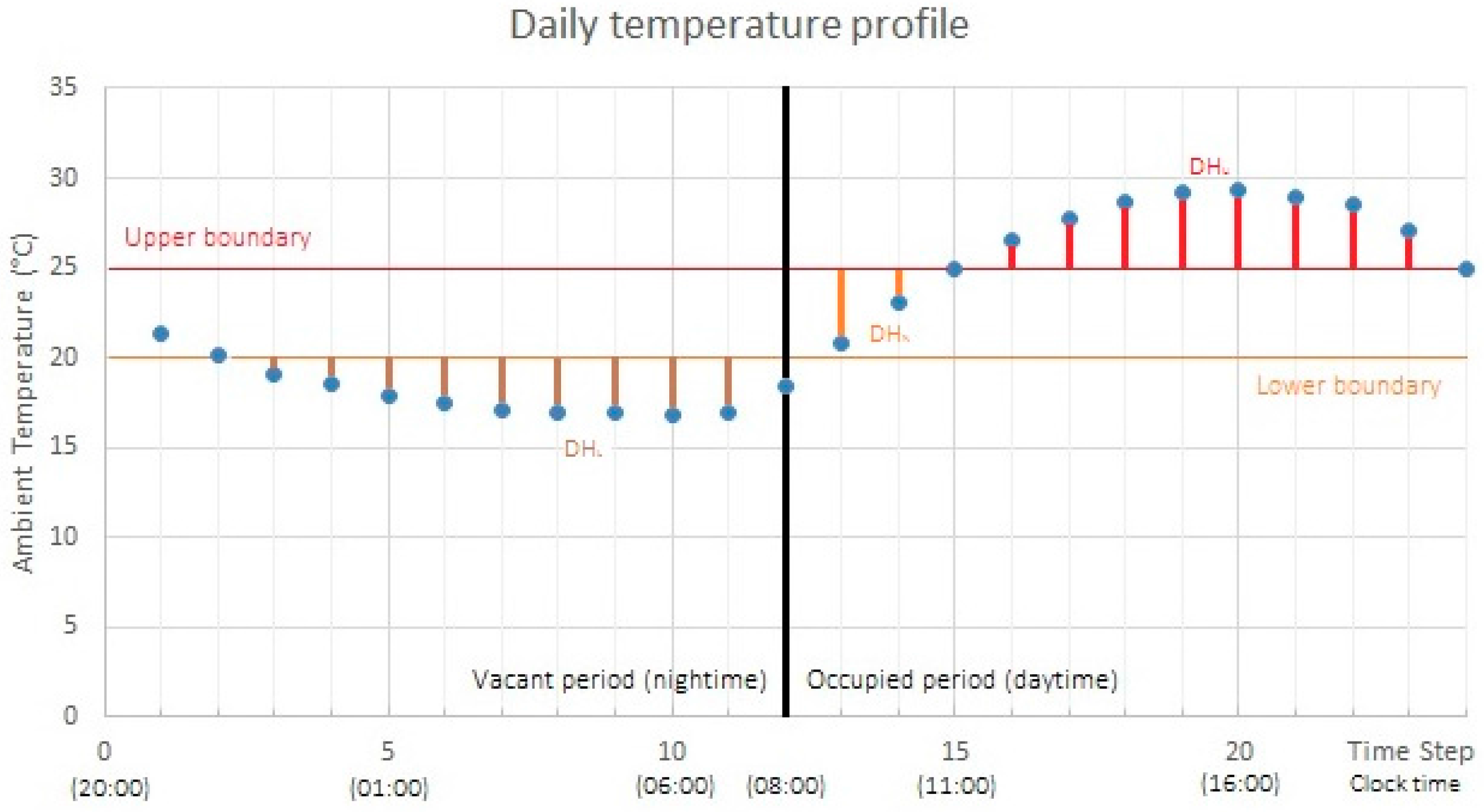
As discussed in Section 2.4.1, the ratio r₁ can be thought of as the precooling potential. In essence it expresses the theoretical percentage of cooling load during the daytime (which is proportional to the DH_U) that may be covered by precooling the night before (which is proportional to the DH_L, assuming precooling infrastructure is in place).

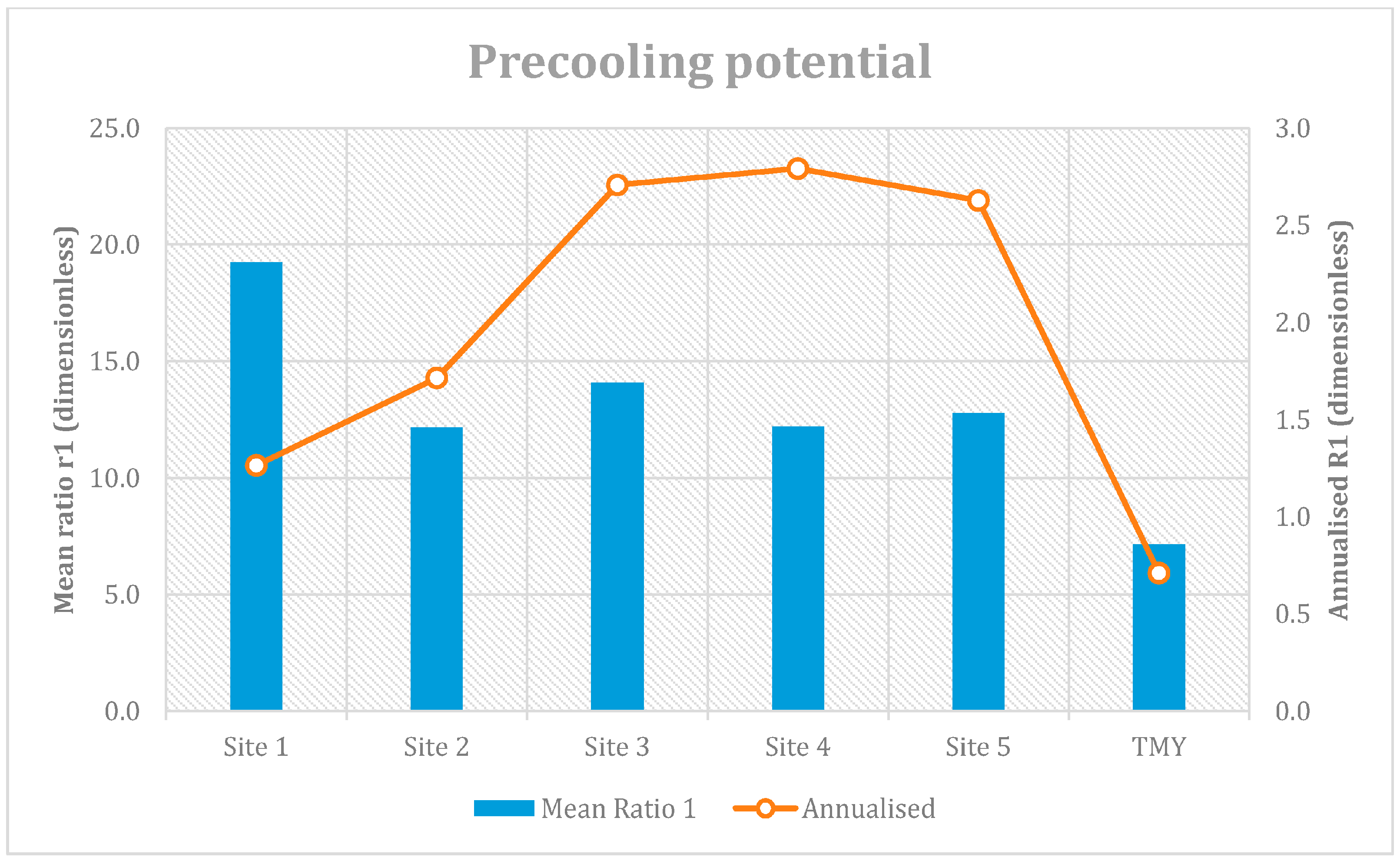
The average precooling potential can be seen in Figure 5. The value of r₁ (before being normalised over a year) shows that the potential for precooling is significant across all sites. In fact the r₁ range is between 12 and 19.25, which implies that on average there is significant precooling potential even for sites 1 and 2, where the frequency is low.

After annualising by multiplying the precooling potential ratio by the precooling frequency ratio, it was shown in Figure 5 that sites 3, 4 and 5 are associated with the highest precooling potential. This illustrates the value of annualising the proposed ratio in interpreting the results: for instance, site 1 (Bondi), has the highest r₁, and the lowest R₁ among the Sydney sites. This is due to the fact that at site 1 the precooling conditions do not occur that often in a typical year, however when they do the diurnal temperature differences are rather high (hence high r₁). Site 2 has much lower r₁, which implies that when the precooling conditions are met, the potential is not great—however, it occurs more frequently than in site 1 in a typical year. On the contrary, and while the average r₁ for the inland sites (3, 4 and 5) is lower than in site 1, the overall yearly precooling potential is much more significant, as the conditions are met more often. 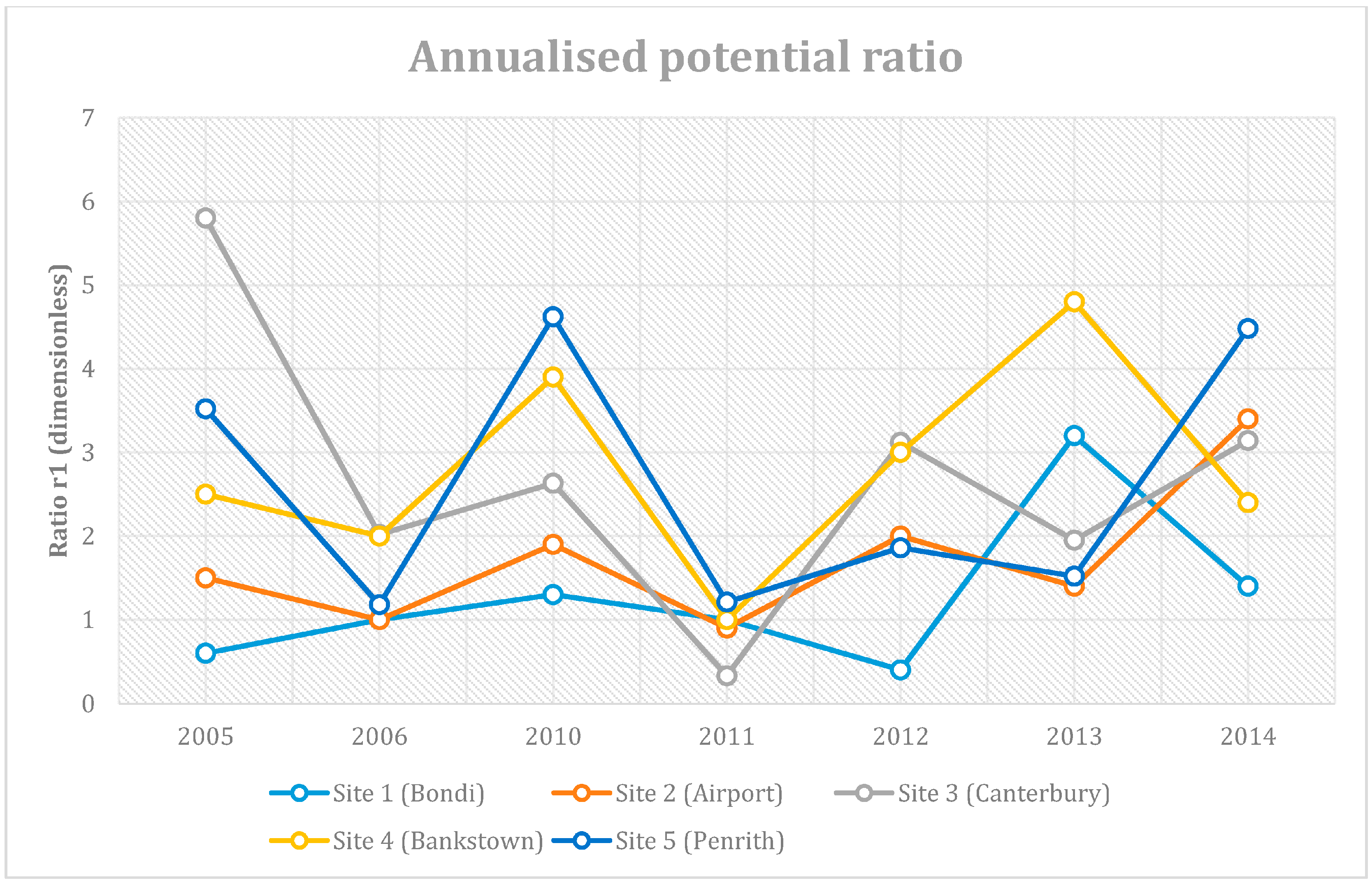As seen in Figure 6, the gradients over the simulation years are not as consistent as with precooling frequency. Regardless, certain features are still evident, such as that all sites had low potential for precooling in 2011 (due to relatively low diurnal temperature differences in the region).

3.4. Precooling Utilisation

The potential ratio by itself is not sufficient to make solid conclusions about the precooling value. While high values of ratio r₁ imply that there is potential for precooling, it may be the result of a low number of degree-hours that actual cooling is needed (denominator of r₁). In simple terms, this would refer to situations that cool nights are followed by relatively mild days, with only a few degree-hours over the upper comfort zone boundary. In such cases, the peak heating would be negligible, however the ratio r₁ would indicate a high potential.

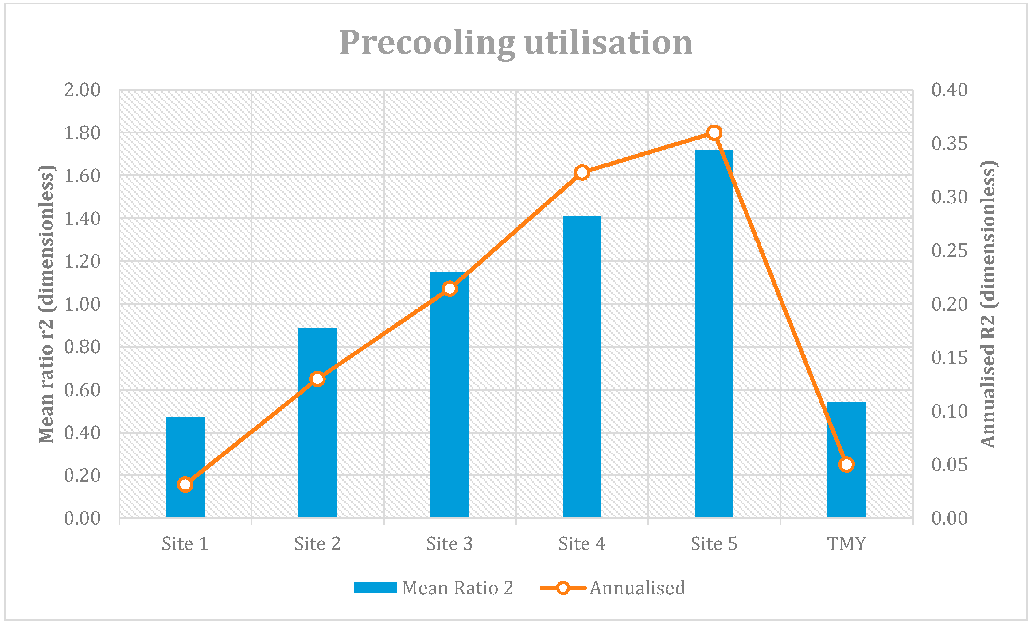
The utilisation ratio r₂ shows the overall utilisation of precooling potential. Figure 7 shows the utilisation ratios for all sites as well as the TMY data, including the mean values and the annualised values. Both the mean r₂ and annualised R₂ display a more consistent pattern than the precooling potential.

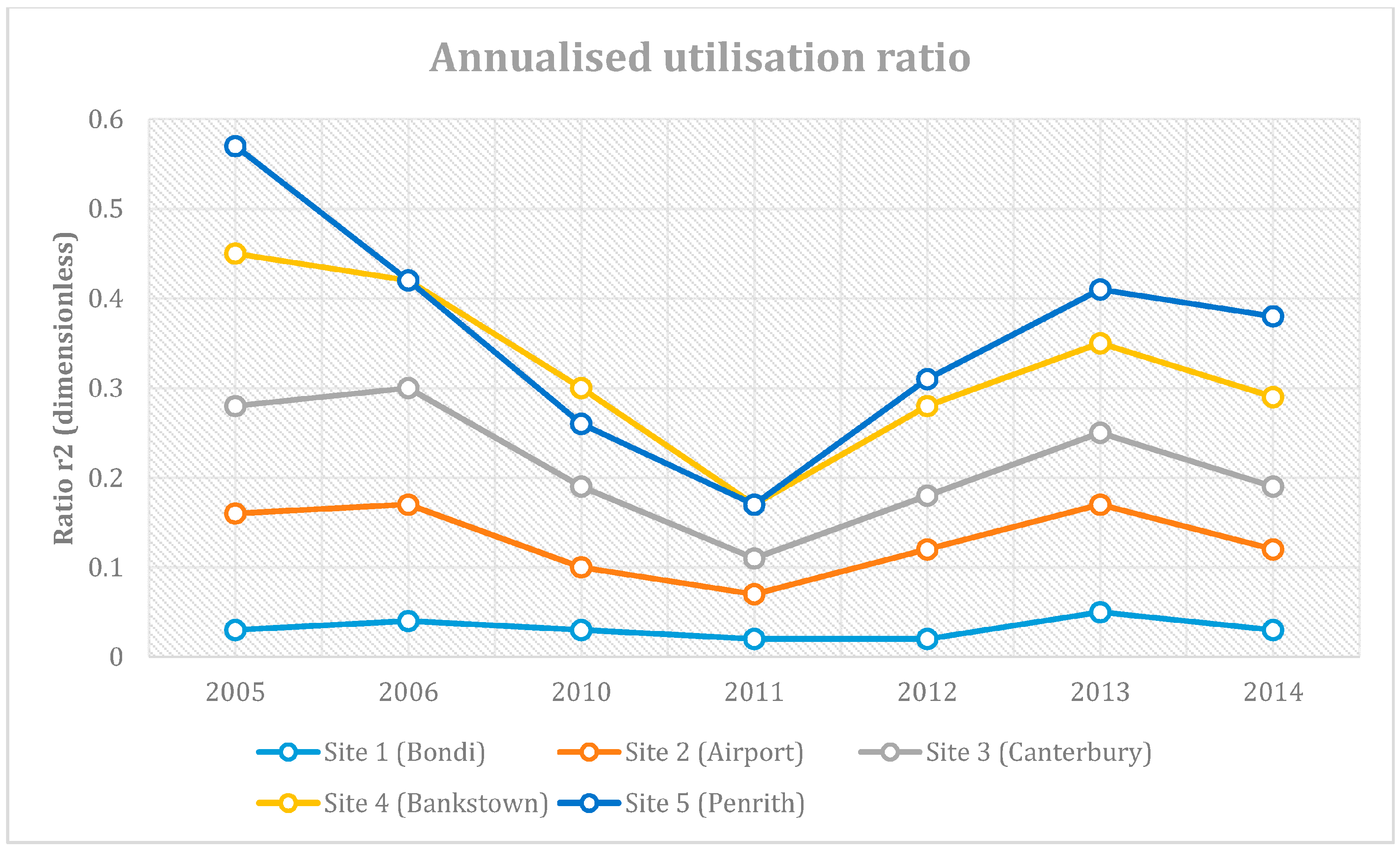
This trend is also visible in Figure 8, which shows a comparison of the annualised utilisation ratios for each year and each site in the simulations. Over the years, there is a consistent assessment of precooling utilisation across all sites.

3.5. Precooling Value

The results showing the median theoretical precooling value for each year, as well as the average theoretical precooling value of seven years’ worth of simulations can be seen in

Table 7. Summary of precooling value ratios for the five sites in Sydney.

Site	2005	2006	2010	2011	2012	2013	2014	Average Value
Site 1	−2.89	−1.73	−3.40	−4.03	−1.70	−1.25	−2.10	−2.44
Site 2	−0.42	−0.07	−0.21	−0.49	−0.64	−0.03	−0.34	−0.31
Site 3	0.16	0.23	0.04	−0.12	−0.14	0.01	0.09	0.04
Site 4	0.16	0.22	0.04	0.00	0.03	0.22	0.19	0.12
Site 5	0.29	0.35	0.01	0.03	0.11	0.27	0.23	0.18

.

Sites 4 (Bankstown) and 5 (Penrith) display a positive theoretical precooling value and more importantly, consistently positive results for the years considered. On the other hand, sites 1 (Bondi) and 2 (Airport) have negative average values, with individual years being negative as well. This implies that sites 4 and 5 possess the potential for a building to utilise natural precooling with meaningful savings, while the savings will be negligible for buildings in sites 1 and 2. Site 3 (Canterbury) has a positive average theoretical precooling value, however as seen in specific years with lower diurnal temperature differences (such as 2011–2012) the savings are expected to be negligible. Hence, site 5 (Penrith) was the best performing site according to the analysis in this chapter and it is expected that whenever precooling conditions are met there is a theoretical average of 18% coverage of the cooling loads via precooling.

Of course the exact savings by the precooling process depend largely on the actual building characteristics and infrastructure. The results of the simulations in this chapter can serve as a preliminary assessment for the value that is realised at a specific location, regardless of building type.

3.6. Precooling Dependence on Local Climate Factors

As stated in the beginning of the paper, the development of the proposed tool may help in obtaining useful insight on the effects of climate patterns on different aspects of precooling processes. Certain trends in climate may cause “irregular” results to appear in the simulations, which can be realised as significant deviations of the precooling ratios from the average values (outliers). The precooling ratios as well as the frequency depend on the diurnal temperature differences. The magnitude of diurnal temperature differences (between maximum and minimum temperatures) is of particular importance and needs to be considered in addition to the actual observed values to characterise the potential of a site.

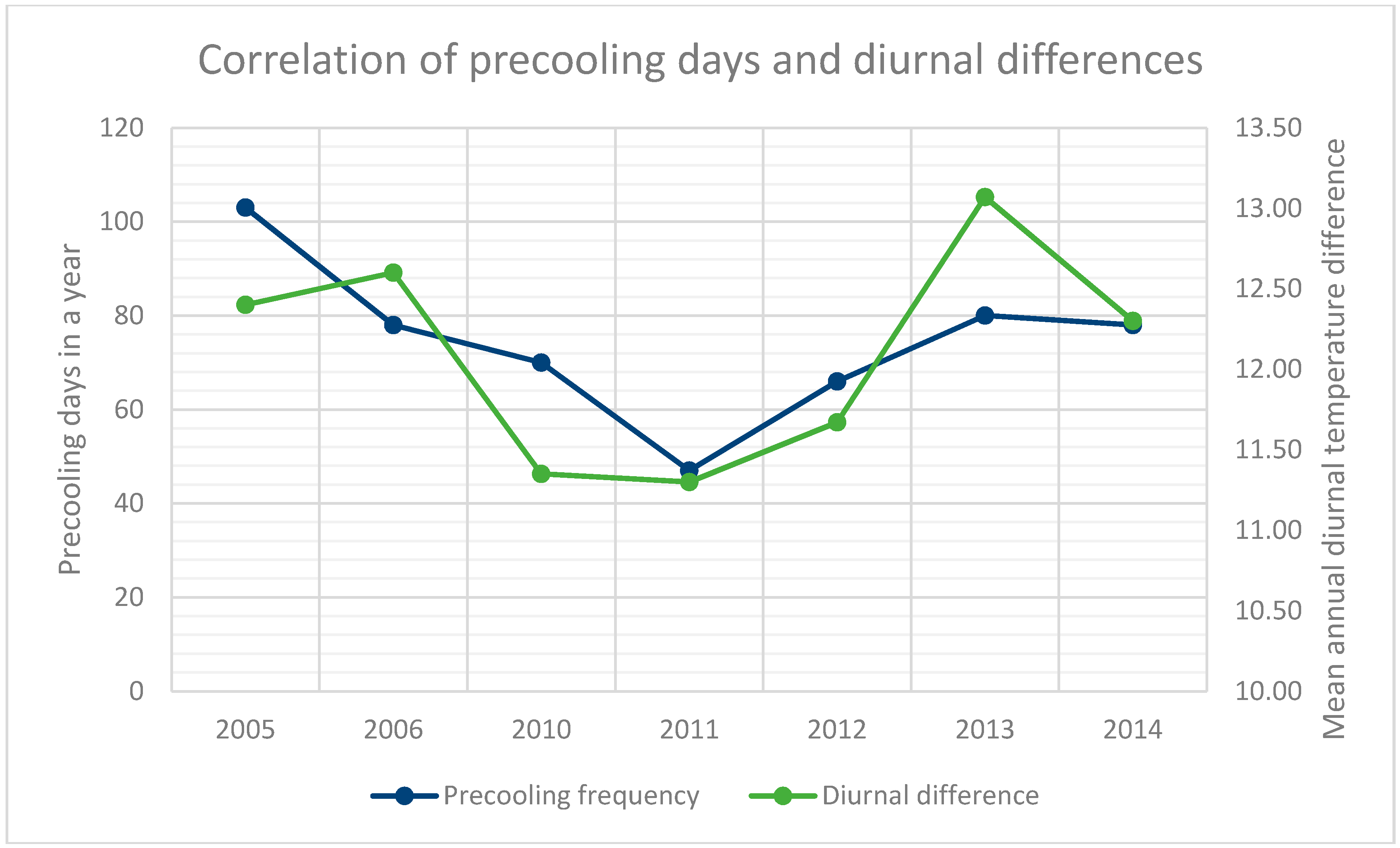
In general, it was found that if the diurnal temperature difference is larger than normal, the precooling frequency and utilisation would improve. Accordingly the theoretical value of precooling would improve as well. The reason for this is that more natural cooling is available overnight and higher cooling loads the day after. To illustrate this effect, the mean monthly diurnal temperature differences for site 5 (Penrith) were compared for the simulation years. The value was calculated as the mean maximum temperature for that month minus the respective mean minimum temperature. The comparison data was obtained from an independent source (Bureau of Meteorology [41]) to eliminate model bias. The comparison was carried out for the months of the year that precooling is possible (summer). The results are displayed in

Table 8. Comparison of mean monthly diurnal temperature differences for each simulation year and 20 year average for Penrith.

Month	Average	2014	2013	2012	2011	2010	2006	2005
October	13.8	14.8	17.6	15.2	11.7	12.1	15.1	12.7
November	12.3	13.8	12.7	12.3	12	10.7	15.1	10.5
December	12.3	11.3	13.7	12.4	9.7	11.2	13	15.7
January	12.3	13.4	12.8	11.1	12.3	12.7	10.1	11.5
Febuary	10.8	10.6	10	9.4	11.9	10.6	11.8	10.7
March	10.9	9.9	11.6	9.6	10.2	10.8	10.5	8.5
Annual	12.07	12.30	13.07	11.67	11.30	11.35	12.60	11.60

.

Figure 9 shows the correlation between precooling frequency in site 5 and the magnitude of diurnal temperature differences for each year. It can be seen that for 2011, during which the frequency (as well as precooling utilisation) were lower than the rest of the simulation years, the mean diurnal difference for the precooling months was the lowest as well. This climate anomaly in 2011 was mainly due to December maximum temperatures being significantly lower than average [41]. It is worth noting that the absolute magnitude of the maximum and minimum temperatures, as well as the weighting of each month to precooling can be considered to improve the accuracy of estimating the correlation between frequency and diurnal differences.

The findings from the simulations confirm the expected results stated in the beginning of this paper; high diurnal temperatures are indeed the primary factor for precooling potential and even within a relatively short distance, diurnal temperatures may vary by a notable extent. In the next section, the findings are generalised for various climatic regimes across Australia.

3.7. Simulations for Different Climates

The precooling assessment tool analysis showed that the five sites across Sydney demonstrate different characteristics. Overall, inland sites within a similar climate were proven superior for precooling. For sites closer to the coast, diurnal temperature differences are moderated by the effects of the heat stored in the ocean. Furthermore, breezes from the open sea may act to reduce the maximum temperatures at coastal sites during a hot day compared to an inland site. These effects were visible in the results for both the precooling frequency and value.

Hence, it is expected that the difference in results will be even more notable when applying the model in climates that are significantly different to Sydney. For the analysis in this section, five Australian cities were considered.

Melbourne, Victoria has a slightly different climate compared to Sydney with higher temperatures during the summer and lower temperatures during the winter. The diurnal differences are expected to be larger, hence resulting in higher precooling potential and value.

On the other hand, Brisbane, Queensland has a subtropical climate with milder temperature gradients and warmer summer nights. Hence it is expected that the precooling potential will be lower compared to Sydney.

Canberra is relatively close to Sydney, but the climate is significantly different, as it is located in the middle of a valley, 70 km inland and an elevation of approximately 580 m. Due to its continental climate, high vegetation coverage, low density and geographical features it is expected to demonstrate high precooling potential.

Alice Springs in the Northern Territory is a city located in a dry desert climate more than 1000 km from the coast. Typically, due to high radiation of desert overnight and high solar exposure during the day, diurnal differences are expected to be rather high in such an environment.

For all cities the simulations were carried out at locations relatively close to the ocean, where applicable (less than 2 km), and compared with a similar location in Sydney (site 2—Airport) in

Table 9. Comparison of precooling potential in different climates.

	Sydney	Melbourne	Brisbane	Canberra	Alice Springs
Climate type (Köppen classification)	Temperate oceanic	Temperate oceanic	Humid Subtropical	Continental	Desert
Ratio h	0.14	0.18	0.01	0.19	0.34
Annual Precool days	52	66	4	69	124
Annualised R1	1.71	3.96	0.03	5.83	9.53
Annualised R2	0.13	0.59	0	0.45	0.91
Precooling value	−0.31	1.26	−9.46	1.42	0.17

.

As seen in Table 9, the assumptions from considering the different climates and geographical locations of each capital are confirmed by the results of the simulations. For Melbourne, the average precooling value of 1.26 implies that natural precooling is theoretically able to cover 100% of the cooling loads on certain days. As with Melbourne, Canberra has the potential for excellent precooling value, with theoretical 100% coverage of cooling loads around 19% of the year. The utilisation ratio is lower, since there are in general lower peak temperatures compared to Melbourne.

On the other hand, Brisbane does not display any realistic precooling potential with a negligible amount of precooling days and very low precooling value. Finally, Alice Springs demonstrated some interesting results. The ratios for the precooling frequency, potential and utilisation are much higher than other cities, due to the significant magnitude of diurnal temperature differences. However, the precooling value is not as high since the daytime temperatures are much higher for longer periods of time during the precooling days, resulting in a high denominator in the value ratio.

4. Discussion and Conclusions

Precooling is recognised as a sustainable solution for the optimisation and management of energy performance of commercial buildings through the reduction of energy consumption and peak shaving. Precooling a building is a low cost solution as it utilises the diurnal temperature differences to manage energy demand with appropriate infrastructure. Actively managed HVAC operations can be applied regardless of the prevalent weather conditions, but nevertheless depend on the diurnal temperature differences as well. In the literature, there are plenty of studies modelling the building performance and savings through such strategies in specific buildings, however there is a lack of studies related to the effects of the location and climate on precooling.

Hence, the proposed tool was able to assess the potential of precooling at a given location. The tool is expected to be a useful option for building designers and energy managers as it may be integrated in decision making for implementing certain preconditioning related features or policies in any location.

The model is based on numerical simulations from a mesoscale weather prediction model—TAPM, and the development of four dimensionless ratios for easy comparison between various sites and climates. The results from the simulations suggest that locations with different characteristics across the same metropolitan area display different potential for natural precooling according to their proximity to the ocean, building density and landscape roughness. The findings also confirm that the precooling process is favoured by high diurnal temperature differences in the summer. Inland sites with high vegetation index and relatively low building density displayed the highest precooling potential and value, due to high diurnal temperature differences that occur frequently in such locations.

The proposed tool is unique in existing literature, as it is the first of its kind utilising numerical climate analysis to assess the potential of precooling, independently of the building characteristics. Any historical weather data could be used as input for the algorithm, however such data are most often not readily available for most locations. TMY or nearby weather station data could be used as an alternative, but the proposed tool provides a more accurate assessment of the precooling value, as it accounts for localised effects of the climate and landscape; it was shown that even sites separated by distances of a few kilometres have significantly difference precooling performance. Depending on the local geography and climatology, TMY data may not be as effective in studies or models for the evaluation of the effects of weather in energy performance of a building. The precooling assessment of a location via TAPM has the additional advantage of being part of a broader range of prediction and characterisation algorithms aiding in short term forecasting, ensemble forecasting and building parameter estimation. Future research may enhance the relevance to precooling predictions by introducing analysis of the effects of relative humidity. Relative humidity affects the enthalpy of air, which in many cases is a more indicative measure of precooling potential than temperature alone.

References

1. Pérez-Lombard, L.; Ortiz, J.; Pout, C. A review on buildings energy consumption information. Energy Build. 2008, 40, 394–398. [Google Scholar] [CrossRef]
2. Lu, N.; Taylor, T.; Jiang, W.; Correia, J.; Leung, L.R.; Wong, P.C. The temperature sensitivity of the residential load and commercial building load. In Proceedings of the IEEE Power & Energy Society General Meeting (PES ′09), Calgary, AB, Canada, 26–30 July 2009; pp. 1–7.
3. Lazos, D.; Sproul, A.B.; Kay, M. Optimisation of energy management in commercial buildings with weather forecasting inputs: A review. Renew. Sustain. Energy Rev. 2014, 39, 587–603. [Google Scholar] [CrossRef]
4. Zhao, H.-X.; Magoulès, F. A review on the prediction of building energy consumption. Renew. Sustain. Energy Rev. 2012, 16, 3586–3592. [Google Scholar] [CrossRef]
5. Steinfeld, J.; Bruce, A.; Watt, M. Peak load characteristics of Sydney office buildings and policy recommendations for peak load reduction. Energy Build. 2011, 43, 2179–2187. [Google Scholar] [CrossRef]
6. Rabl, A.; Norford, L.K. Peak load reduction by preconditioning buildings at night. Int. J. Energy Res. 1991, 15, 781–798. [Google Scholar] [CrossRef]
7. Lazos, D.; Sproul, A.B.; Kay, M. Development of hybrid numerical and statistical short term horizon weather prediction models for building energy management optimisation. Build. Environ. 2015, 90, 82–95. [Google Scholar] [CrossRef]
8. Hurley, P. Verification of tapm meteorological predictions in the Melbourne region for a winter and summer month. Aust. Meteorol. Mag. 2000, 49, 97–107. [Google Scholar]
9. Hurley, P. Development and verification of TAPM. In Proceedings of the 29th NATO/CCMS International Technical Meeting on Air Pollution Modelling and Its Application, Dordrecht, The Netherlands, 24–28 September 2007.
10. Hurley, P.J.; Physick, W.L.; Luhar, A.K. TAPM: A practical approach to prognostic meteorological and air pollution modelling. Environ. Model. Softw. 2005, 20, 737–752. [Google Scholar] [CrossRef]
11. Luhar, A.K.; Hurley, P.J. Application of a prognostic model TAPM to sea-breeze flows, surface concentrations, and fumigating plumes. Environ. Model. Softw. 2004, 19, 591–601. [Google Scholar] [CrossRef]
12. May-Ostendorp, P.; Henze, G.P.; Corbin, C.D.; Rajagopalan, B.; Felsmann, C. Model-predictive control of mixed-mode buildings with rule extraction. Build. Environ. 2011, 46, 428–437. [Google Scholar] [CrossRef]
13. Karava, P.; Athienitis, A.K.; Stathopoulos, T.; Mouriki, E. Experimental study of the thermal performance of a large institutional building with mixed-mode cooling and hybrid ventilation. Build. Environ. 2012, 57, 313–326. [Google Scholar] [CrossRef]
14. Braun, J.E.; Zhong, Z. Development and evaluation of a night ventilation precooling algorithm. HVAC R Res. 2005, 11, 433–458. [Google Scholar] [CrossRef]
15. Peterson, J.L.; Hunn, B.C. Use of indirect evaporative cooling to reduce peak electric demand in new office buildings. ASHRAE Trans. 1985, 91, 329–341. [Google Scholar]
16. Chenvidyakarn, T.; Woods, A. Top-down precooled natural ventilation. Build. Serv. Eng. Res. Technol. 2005, 26, 181–193. [Google Scholar] [CrossRef]
17. Cole, W.J.; Powell, K.M.; Hale, E.T.; Edgar, T.F. Reduced-order residential home modeling for model predictive control. Energy Build. 2014, 74, 69–77. [Google Scholar] [CrossRef]
18. Roth, K.; Dieckmann, J.; Brodrick, J. Using off-peak precooling. ASHRAE J. 2009, 51, 80–83. [Google Scholar]
19. Keeney, K.R.; Braun, J.E. Application of building precooling to reduce peak cooling requirements. In Proceedings of the 1997 American Society of Heating Refrigerating and Airconditioning Engineer (ASHRAE) Winter Meeting, Philadelphia, PA, USA, 24–28 February 1997; pp. 463–469.
20. Lee, K.-H.; Braun, J.E. Reducing peak cooling loads through model-based control of zone temperature setpoints. In Proceedings of the 2007 American Control Conference (ACC), New York, NY, USA, 9–13 July 2007; Institute of Electrical and Electronics Engineers Inc.: New York, NY, USA, 2007; pp. 5070–5075. [Google Scholar]
21. Greensfeldera, E.M.; Henzea, G.P.; Felsmannb, C. An investigation of optimal control of passive building thermal storage with real time pricing. J. Build. Perform. Simul. 2011, 4, 91–104. [Google Scholar] [CrossRef]
22. Lockerbie, J. The Use of Thermal Mass. Available online: http://catnaps.org/islamic/approach3.html (accessed on 22 May 2016).
23. Hu, J.; Karava, P. Model predictive control strategies for buildings with mixed-mode cooling. Build. Environ. 2014, 71, 233–244. [Google Scholar] [CrossRef]
24. Kruger, E.; Fernandes, L. Error analysis of temperature predictions for the indoor temperature in low-cost houses. In Proceedings of the 22nd Conference on Passive and Low Energy Architecture, Beirut, Lebanon, 13–16 November 2005.
25. Spindler, H.C.; Norford, L.K. Naturally ventilated and mixed-mode buildings—Part I: Thermal modeling. Build. Environ. 2009, 44, 736–749. [Google Scholar] [CrossRef]
26. Rasouli, M.; Gaoming, G.; Simonson, C.J.; Besant, R.W. Uncertainties in energy and economic performance of HVAC systems and energy recovery ventilators due to uncertainties in building and HVAC parameters. Appl. Therm. Eng. 2013, 50, 732–742. [Google Scholar] [CrossRef]
27. Kintner-Meyer, M.; Emery, A.F. Optimal control of an HVAC system using cold storage and building thermal capacitance. Energy Build. 1995, 23, 19–31. [Google Scholar] [CrossRef]
28. Todhunter, P.E.; Terjung, W.H. Intercomparison of three urban climate models. Bound. Layer Meteorol. 1988, 42, 181–205. [Google Scholar] [CrossRef]
29. Santamouris, M.; Papanikolaou, N.; Livada, I.; Koronakis, I.; Georgakis, C.; Argiriou, A.; Assimakopoulos, D.N. On the impact of urban climate on the energy consumption of buildings. Sol. Energy 2001, 70, 201–216. [Google Scholar] [CrossRef]
30. Eichhorn, J.; Schrodin, R.; Zdunkowski, W. Three-dimensional numerical simulations of the urban climate. Contrib. Atmos. Phys. 1988, 61, 187–203. [Google Scholar]
31. Khaled, N.; Krarti, M. Impact of precooling control on reducing electrical peak demand for commercial buildings in tuniisia. In Proceedings of the 2007 Energy Sustainability Conference, Long Beach, CA, USA, 27–30 July 2007; pp. 565–572.
32. Peng, X.; Rongxin, Y.; Carrie, B.; DongEun, K. Demand Shifting with Thermal Mass in Large Commercial Buildings in a California Hot Climate Zone; California Energy Commission/Lawrence Berkeley National Laboratory: Berkeley, CA, USA, 2009.
33. Briller, D.L. Strategies for optimally managing building peak demand under climate-altered scenarios. In Proceedings of theWorld Energy Engineering Congress 2012 (WEEC 2012), Atlanta, GA, USA, 31 October–2 November 2012; The Fairmont Press, Inc.: Atlanta, GA, USA, 2012; pp. 857–879. [Google Scholar]
34. WorkSafe Victoria. Workplace Amenities and Work Environment—Compliance Code; Victoria State Government: Melbourne, Australia, 2008.
35. Oldewurtel, F.; Parisio, A.; Jones, C.N.; Gyalistras, D.; Gwerder, M.; Stauch, V.; Lehmann, B.; Morari, M. Use of model predictive control and weather forecasts for energy efficient building climate control. Energy Build. 2012, 45, 15–27. [Google Scholar] [CrossRef]
36. Havenith, G.; Holmér, I.; Parsons, K. Personal factors in thermal comfort assessment: Clothing properties and metabolic heat production. Energy Build. 2002, 34, 581–591. [Google Scholar] [CrossRef]
37. Day, T. TM41 Degree Days: Theory and Application; Chartered Institution of Building Services Engineers (CIBSE): London, UK, 2006. [Google Scholar]
38. Krese, G.; Prek, M.; Butala, V. Incorporation of latent loads into the cooling degree days concept. Energy Build. 2011, 43, 1757–1764. [Google Scholar] [CrossRef]
39. Layberry, R.L. Degree days for building energy management—Presentation of a new data set. Build. Serv. Eng. Res. Technol. 2008, 29, 273–282. [Google Scholar] [CrossRef]
40. U.S. Department of Energy. EnergyPlus Energy Simulation Software. 2006. Available online: http://apps1.eere.energy.gov/buildings/energyplus/cfm/weather_data3.cfm/region=5_southwest_pacific_wmo_region_5/country=AUS/cname=Australia (accessed on 3 August 2015). [Google Scholar]
41. BOM. Monthly Mean Temperatures. Available online: http://www.bom.gov.au/jsp/ncc/cdio/weatherData/av?p_nccObsCode=36&p_display_type=dataFile&p_startYear=&p_c=&p_stn_num=067113 (accessed on 16 August 2015).
Figure 1. Map of the five Sydney sites.
Energies 10 00021 g001
Figure 2. Daily temperature profile (as simulated) for Penrith between 27 January 20:00 and 28 January 20:00 in 2014. The upper and lower boundaries can be seen at 25 and 20 degrees respectively. The DH for each time step are calculated as the difference from the base temperature at each period.
Energies 10 00021 g002
Figure 3. Number of days that precooling conditions were met per year for each sites.
Energies 10 00021 g003
Figure 4. Average number of days that precooling conditions are met across the five Sydney sites.
Energies 10 00021 g004
Figure 5. Summary of precooling potential across sites in Sydney.
Energies 10 00021 g005
Figure 6. Annualised potential ratio R1 for the Sydney sites for each simulation year.
Energies 10 00021 g006
Figure 7. Precooling utilisation summary for sites across Sydney.
Energies 10 00021 g007
Figure 8. Annualised utilisation ratio (R2) for Sydney sites for each simulation year.
Energies 10 00021 g008
Figure 9. Comparison of precooling days per year and the magnitude of the mean annual diurnal temperature difference.
Energies 10 00021 g009