
Real-Time Velocity Optimization to Minimize Energy Use in Passenger Vehicles


Abstract
:1. Introduction
- Anticipate traffic flow
- Maintain a steady speed at low engine speed
- Shift up early
2. Methodology
2.1. Vehicle Model
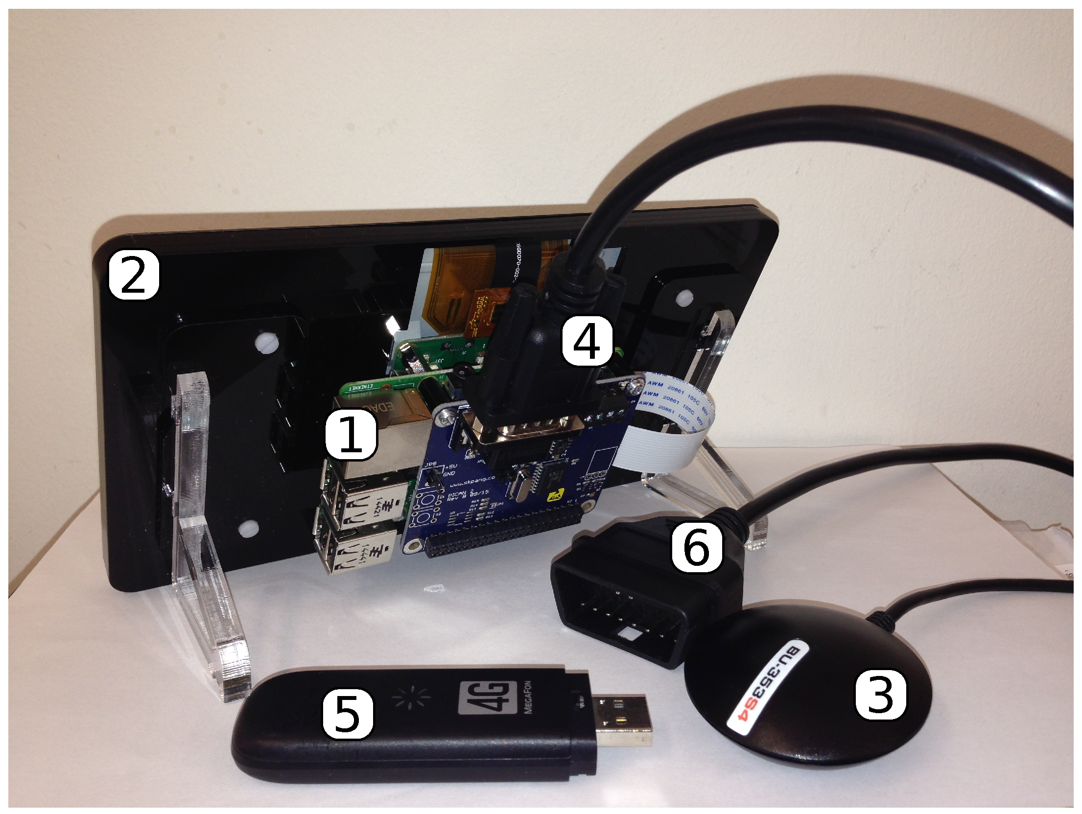
2.2. Hardware
2.3. Software
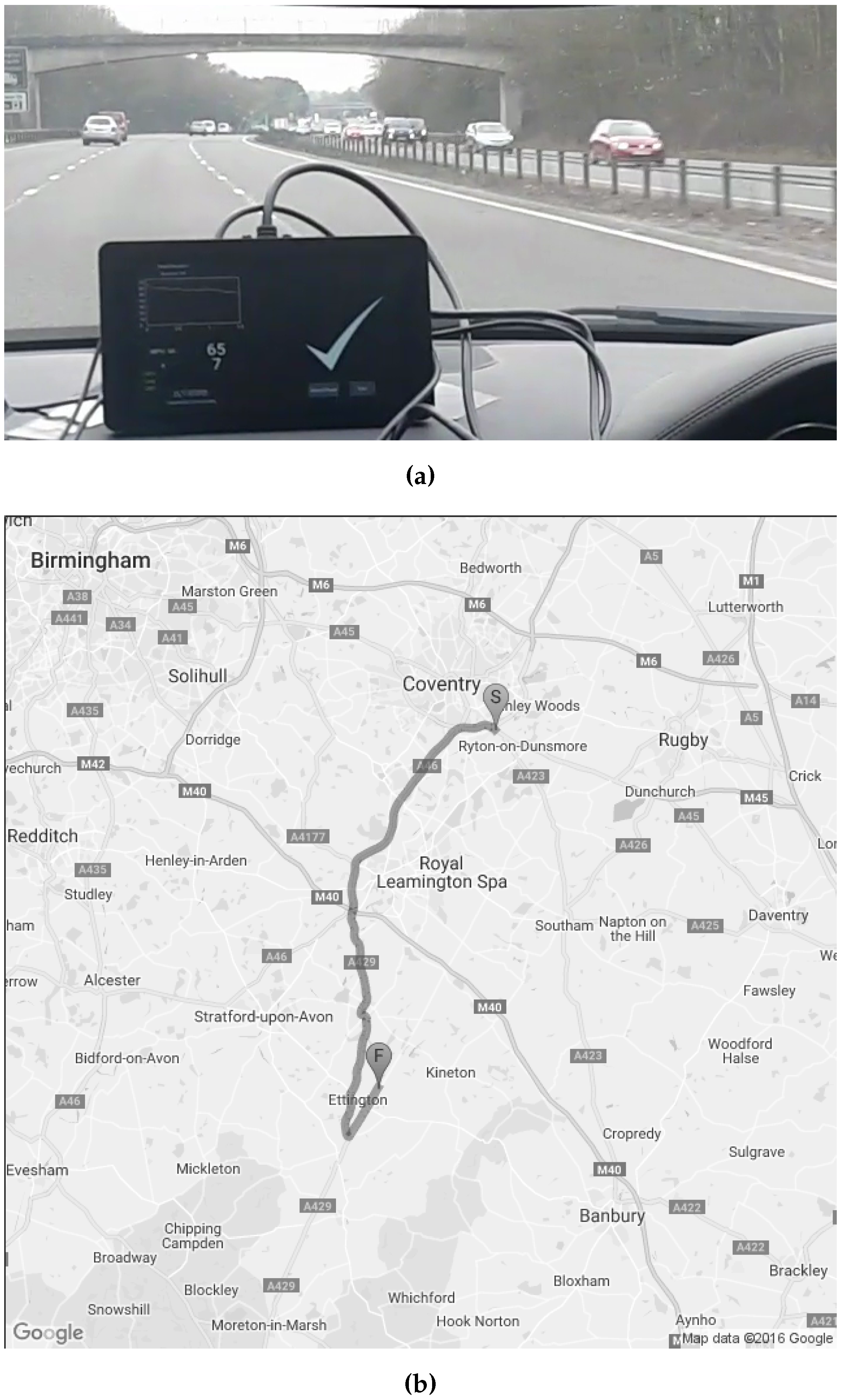
Data Acquisition
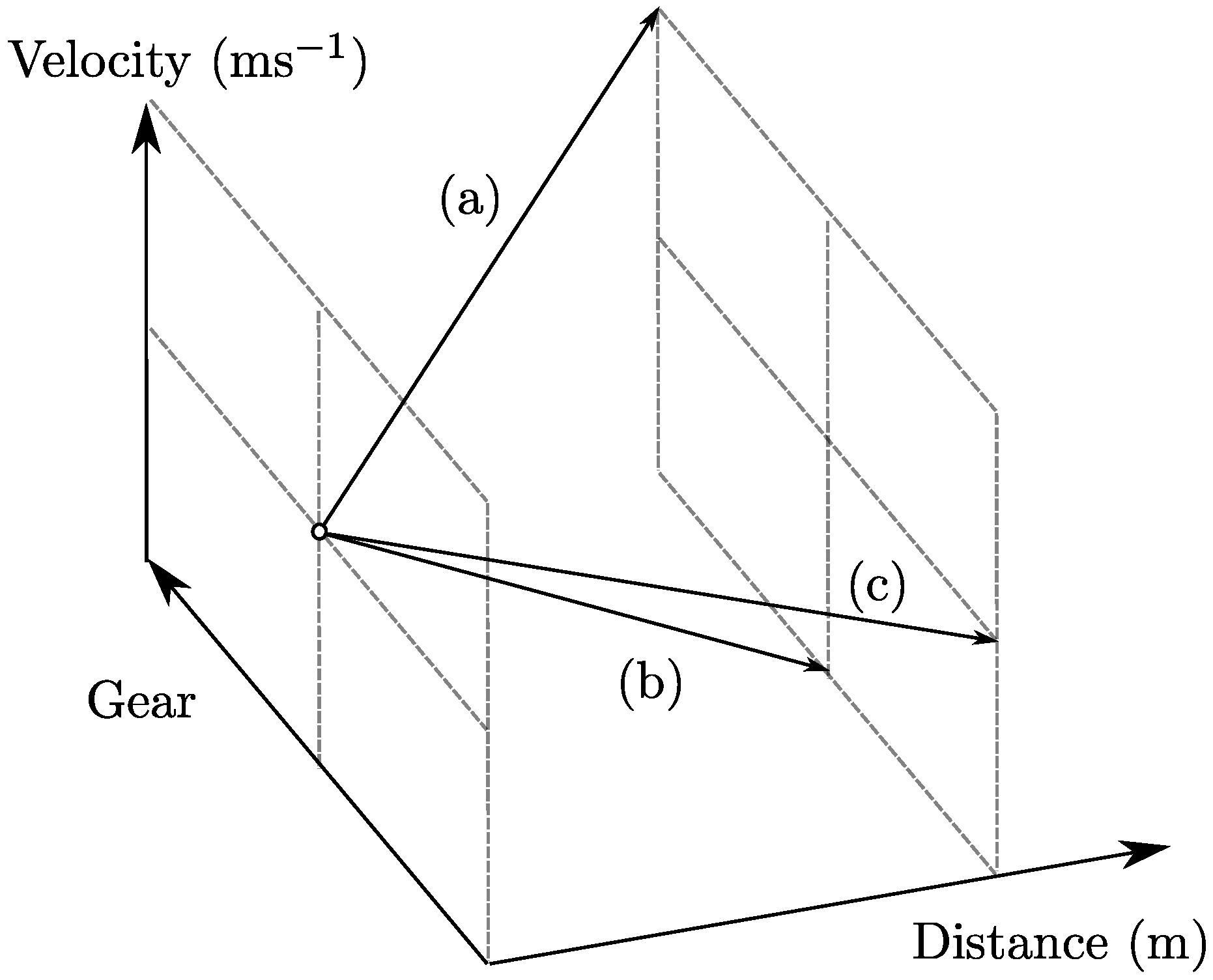
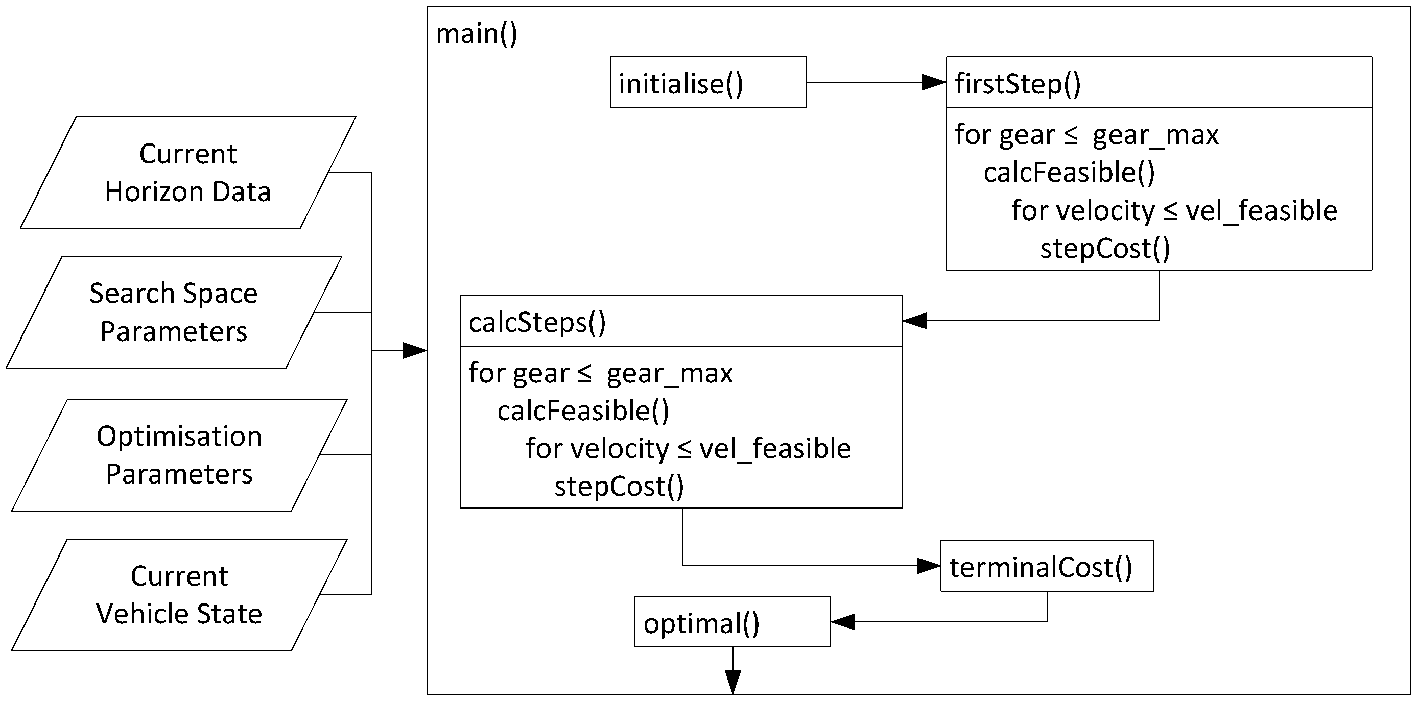
2.4. Algorithm Implementation
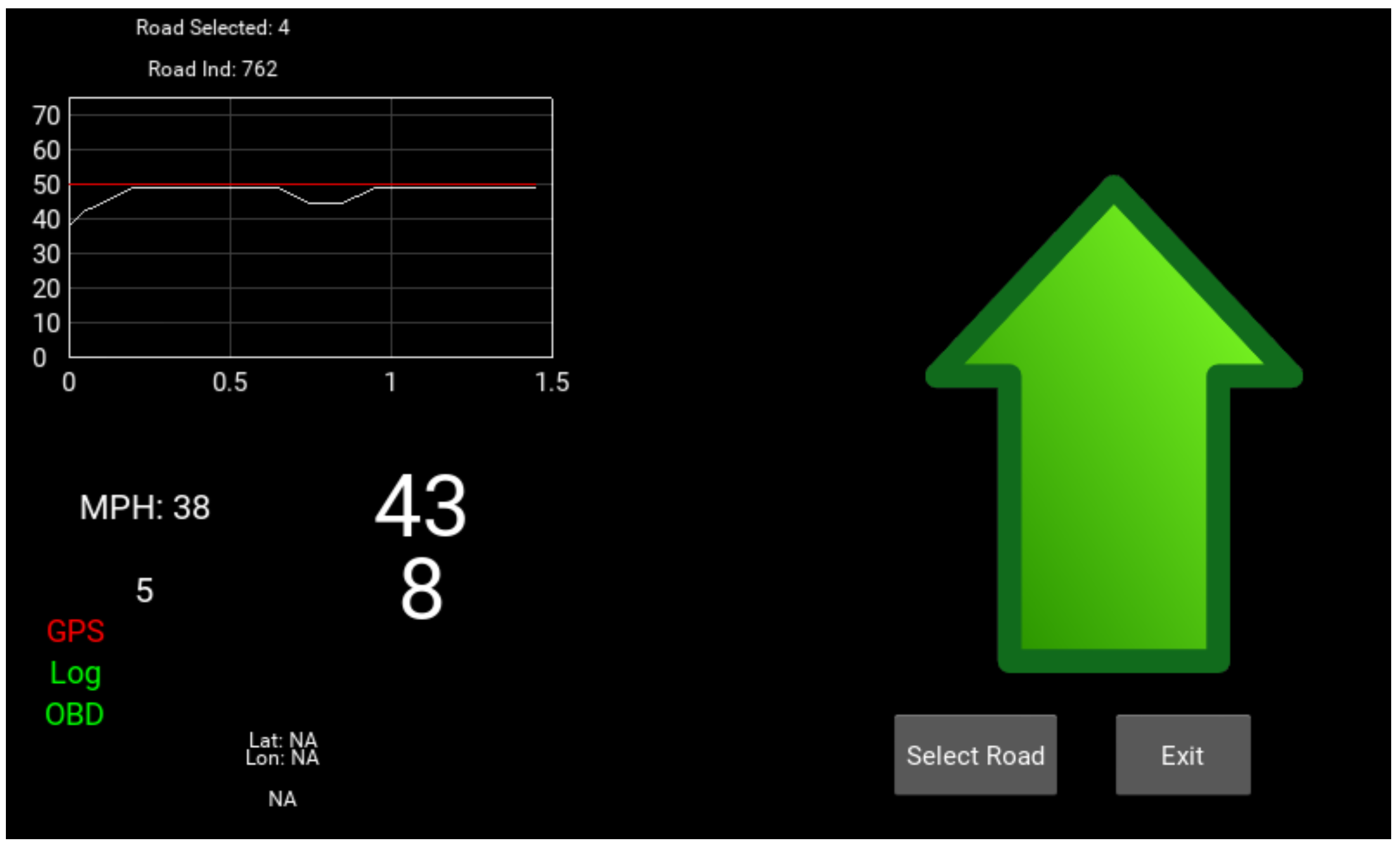
2.5. User Interface
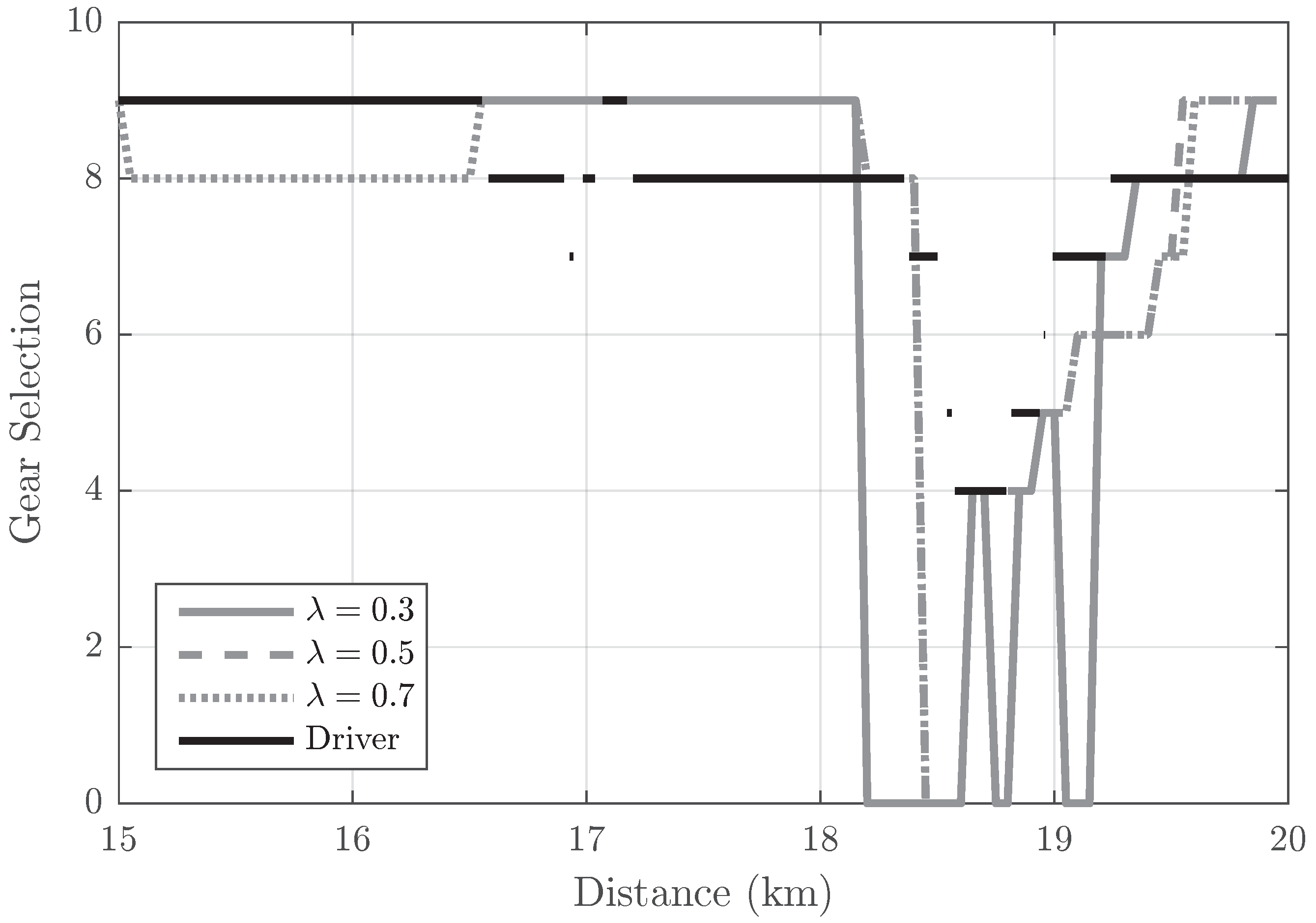
3. Results and Discussion
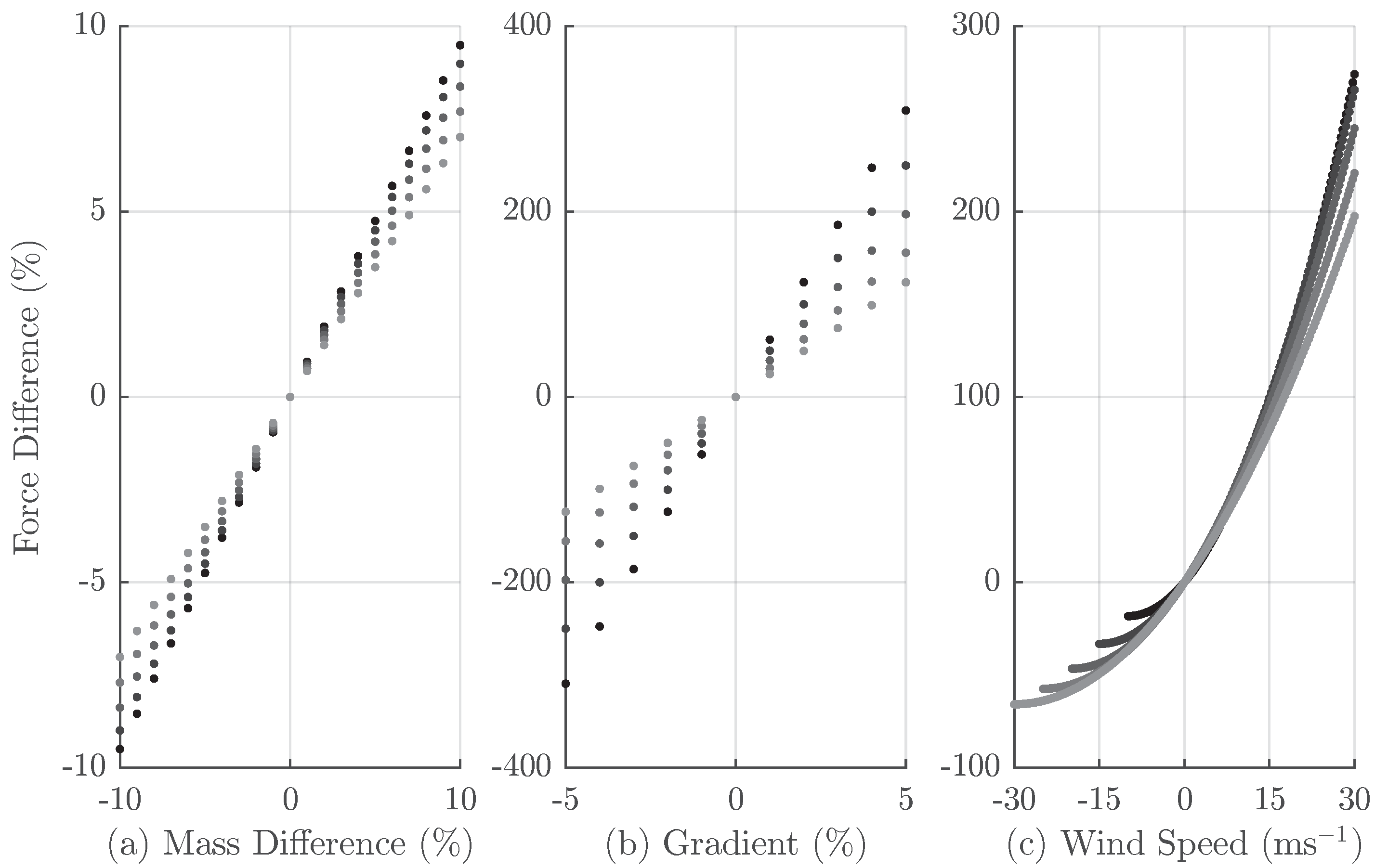
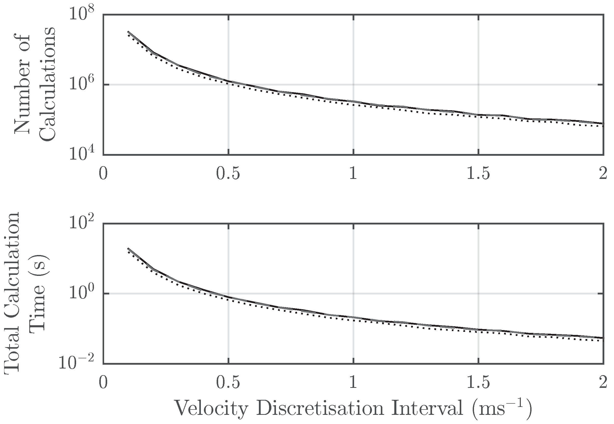
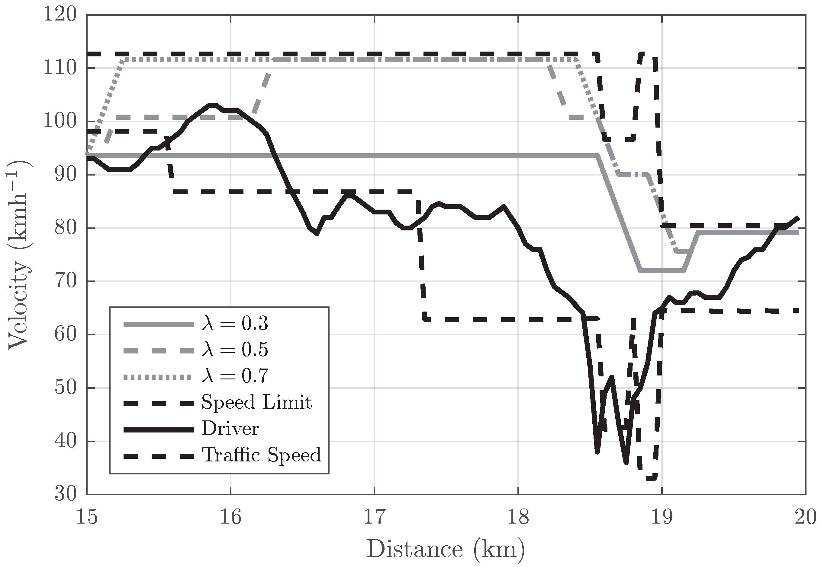
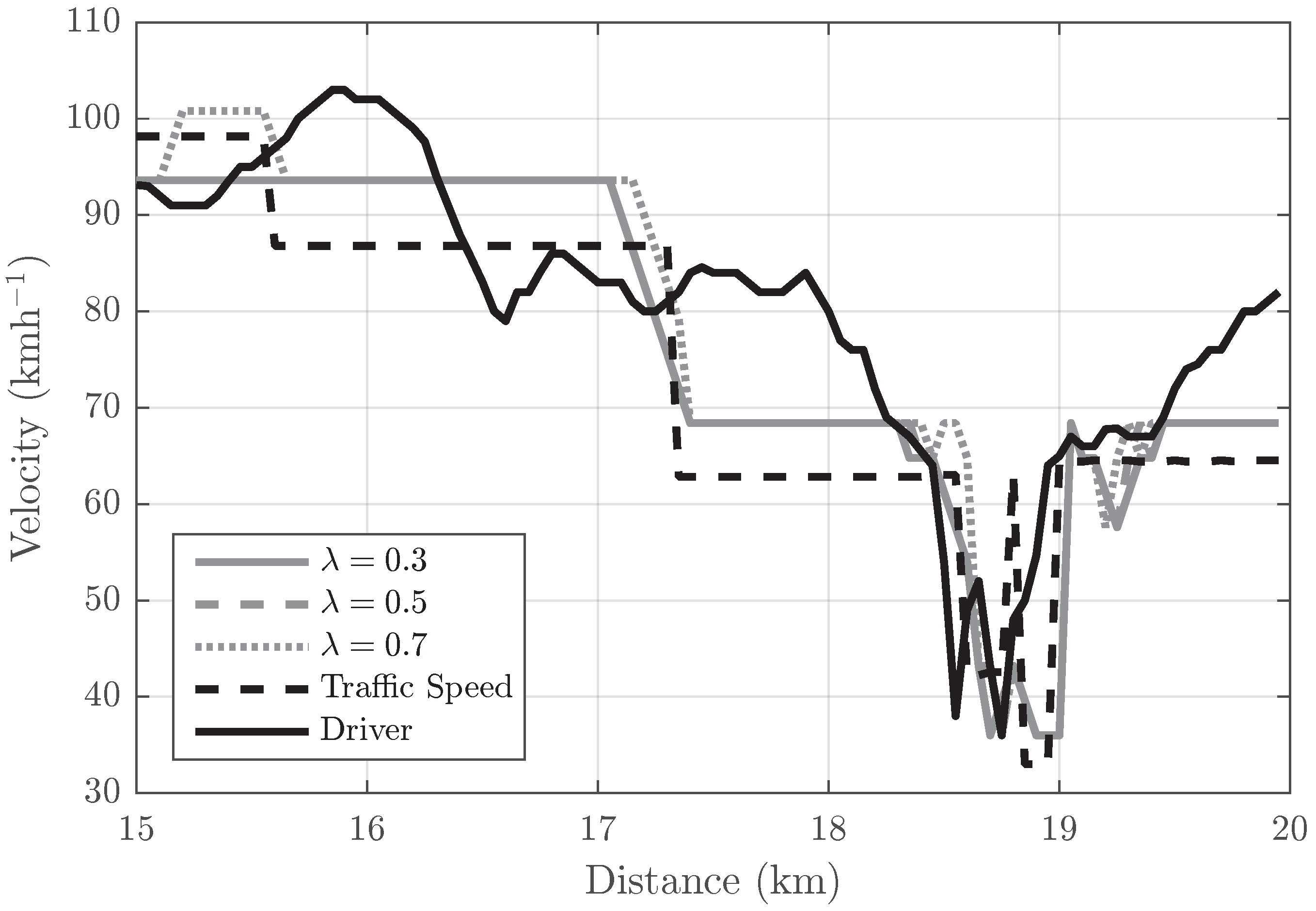
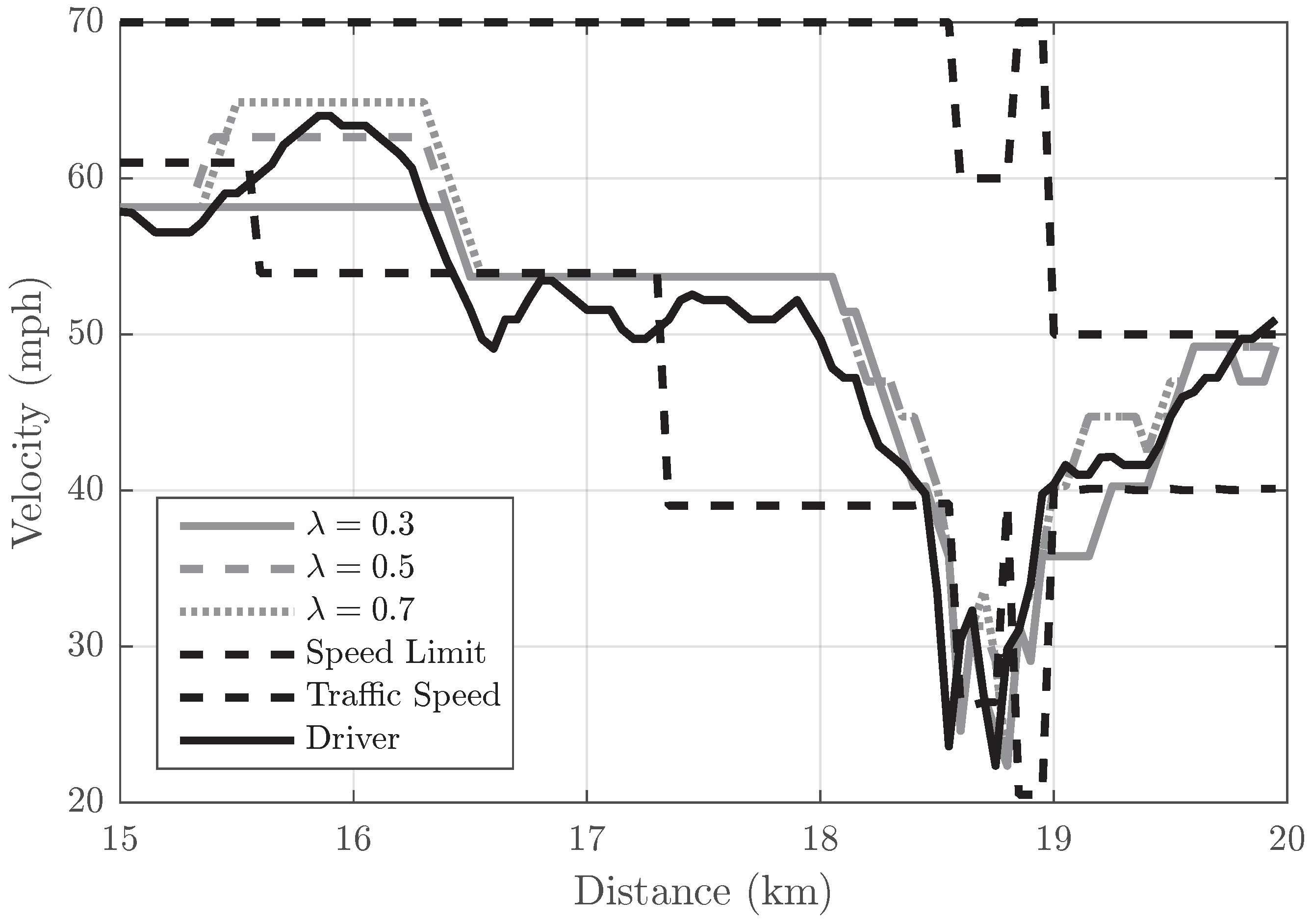
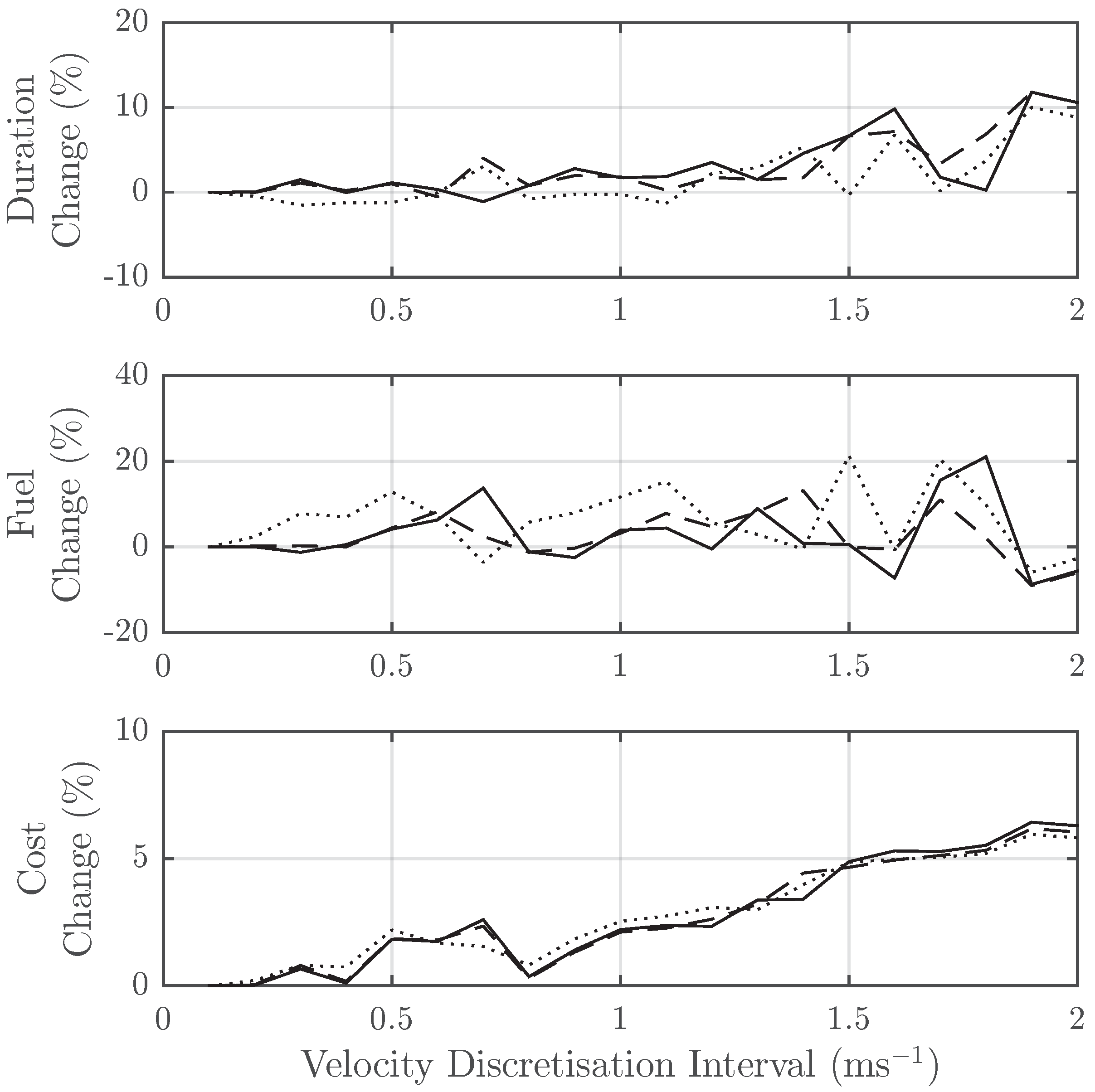
Algorithm Sensitivity
4. Conclusions
Acknowledgments
Author Contributions
Conflicts of Interest
Abbreviations
| BSFC | Brake-Specific Fuel Consumption |
| CAN | Controller Area Network |
| DP | Dynamic Programming |
| HGV | Heavy Goods Vehicle |
| MDPI | Multidisciplinary Digital Publishing Institute |
References
- Stocker, T.; Qin, D.; Plattner, G.; Tignor, M.; Allen, S.; Boschung, J.; Nauels, A.; Xia, Y.; Bex, V.; Midgley, P. Climate Change 2013: The Physical Science Basis; Fifth Assessment Report; Intergovernmental Panel on Climate Change: Geneva, Switzerland, 2013. [Google Scholar]
- International Energy Agency. CO2 Emissions From Fuel Combustion Highlights 2015; Technical Report; International Energy Agency: Paris, France, 2015. [Google Scholar]
- Heywood, J.B. Internal Combustion Engine Fundamentals; McGraw-Hill: New York, NY, USA, 1988. [Google Scholar]
- An, F.; Sauer, A. Comparison of Passenger Vehicle Fuel Economy and Greenhouse Gas Emission Standards Around the World; Center for Climate and Energy Solutions: Arlington, VA, USA, 2004. [Google Scholar]
- Boriboonsomsin, K.; Barth, M.J.; Zhu, W.; Vu, A. Eco-routing navigation system based on multisource historical and real-time traffic information. IEEE Trans. Intell. Transp. Syst. 2012, 13, 1694–1704. [Google Scholar] [CrossRef]
- Minett, P.; Pearce, J. Estimating the energy consumption impact of casual carpooling. Energies 2011, 4, 126. [Google Scholar] [CrossRef]
- Barkenbus, J.N. Eco-driving: An overlooked climate change initiative. Energy Policy 2010, 38, 762–769. [Google Scholar] [CrossRef]
- Hiraoka, T.; Terakado, Y.; Matsumoto, S.; Yamabe, S. Quantitative evaluation of eco-driving on fuel consumption based on driving simulator experiments. In Proceedings of the 16th World Congress on Intelligent Transport Systems, Stockholm, Sweden, 21–25 September 2009; pp. 21–25.
- Beusen, B.; Broekx, S.; Denys, T.; Beckx, C.; Degraeuwe, B.; Gijsbers, M.; Scheepers, K.; Govaerts, L.; Torfs, R.; Panis, L.I. Using on-board logging devices to study the longer-term impact of an eco-driving course. Transp. Res. Part D Transp. Environ. 2009, 14, 514–520. [Google Scholar] [CrossRef]
- ECOWILL Project. Available online: http://www.ecodrive.org/download/downloads/ecowill_brochure.pdf (accessed on 8 January 2016).
- Kock, P.; Ordys, A.; Collier, G.; Weller, R. Intelligent predictive cruise control application analysis for commercial vehicles based on a commercial vehicles usage study. SAE Int. J. Commer. Veh. 2013, 6, 598–603. [Google Scholar] [CrossRef]
- Terwen, S.; Back, M.; Krebs, V. Predictive powertrain control for heavy duty trucks. In Proceedings of the International Federation for Automatic Control (IFAC) Symposium on Advances in Automotive Control, Salerno, Italy, 19–23 April 2004; pp. 451–457.
- Passenberg, B.; Kock, P.; Stursberg, O. Combined time and fuel optimal driving of trucks based on a hybrid model. In Proceedings of the 2009 European Control Conference (ECC), Budapest, Hungary, 23–26 August 2009; pp. 4955–4960.
- Bellman, R. Dynamic Programming; Princeton University Press: Princeton, NJ, USA, 1957. [Google Scholar]
- Hellström, E.; Ivarsson, M.; Aslund, J.; Nielsen, L. Look-ahead control for heavy trucks to minimize trip time and fuel consumption. Control Eng. Pract. 2009, 17, 245–254. [Google Scholar] [CrossRef]
- Wahl, H.G.; Bauer, K.L.; Gauterin, F.; Holzäpfel, M. A real-time capable enhanced dynamic programming approach for predictive optimal cruise control in hybrid electric vehicles. In Proceedings of the 16th International IEEE Conference on Intelligent Transportation Systems (ITSC 2013), Hague, The Netherlands, 6–9 October 2013; pp. 1662–1667.
- Jiménez, F.; Cabrera-Montiel, W.; Tapia-Fernandez, S. System for road vehicle energy optimization using real time road and traffic information. Energies 2014, 7, 3576. [Google Scholar] [CrossRef]
- Wang, X.; He, H.; Sun, F.; Zhang, J. Application study on the dynamic programming algorithm for energy management of plug-in hybrid electric vehicles. Energies 2015, 8, 3225–3244. [Google Scholar] [CrossRef]
- Shen, W.; Yu, H.; Hu, Y.; Xi, J. Optimization of shift schedule for hybrid electric vehicle with automated manual transmission. Energies 2016, 9, 220. [Google Scholar] [CrossRef] [Green Version]
- Bertsekas, D. Dynamic Programming and Optimal Control; Athena Scientific: Belmont, MA, USA, 2005. [Google Scholar]
- Fröberg, A.; Nielsen, L. Dynamic Vehicle Simulation-Forward, Inverse and New Mixed Possibilities for Optimized Design and Control; SAE Technical Paper; SAE International: Warrendale, PA, USA, 2004. [Google Scholar]
- Rajamani, R. Vehicle Dynamics and Control; Springer: New York, NY, USA, 2011. [Google Scholar]
- Monastyrsky, V.; Golownykh, I. Rapid computation of optimal control for vehicles. Transp. Res. Part B Methodol. 1993, 27, 219–227. [Google Scholar] [CrossRef]
- Influx Technology. Available online: http://www.influxtechnology.com/SharedFiles/Documentation/Rebel/Rebel%20XT%20Product%20Flyer.pdf (accessed on 8 January 2016).
- HERE Routing API Developer’s Guide. Available online: https://developer.here.com/rest-apis/documentation/routing (accessed on 8 July 2016).
- Pretschner, A.; Broy, M.; Kruger, I.H.; Stauner, T. Software engineering for automotive systems: A roadmap. In Proceedings of the Future of Software Engineering, Washington, DC, USA, 23–25 May 2007; pp. 55–71.
- Raspberry Pi Touch Display. Available online: https://www.raspberrypi.org/products/raspberry-pi-touch-display/ (accessed on 6 September 2016).
- US GlobalSat Inc. Available online: http://usglobalsat.com/p-688-bu-353-s4.aspx (accessed on 8 July 2016).
- SK Pang Electronics. PiCAN 2 User Guide, version 1.1; SK Pang Electronics: Essex, UK, 2016. [Google Scholar]
- Broy, M.; Kruger, I.H.; Pretschner, A.; Salzmann, C. Engineering automotive software. Proc. IEEE 2007, 95, 356–373. [Google Scholar] [CrossRef]
- GNU Project. Available online: https://gcc.gnu.org/ (accessed on 8 July 2016).
- Python Software Foundation. Available online: https://docs.python.org/2/library/multiprocessing.html (accessed on 28 June 2016).
- Python-CAN SocketCAN. Available online: https://python-can.readthedocs.io/en/latest/interfaces/socketcan.html (accessed on 21 September 2016).
- CAN Specification, v2.0; Robert Bosch GmbH: Gerlingen, Germany, 1991.
- BUSMASTER. Available online: http://www.etas.com/en/products/applications_busmaster.php (accessed on 18 July 2016).
- GPSD Service Daemon. Available online: http://www.catb.org/gpsd/ (accessed on 8 July 2016).
- Robusto, C.C. The cosine-haversine formula. Am. Math. Mon. 1957, 64, 38–40. [Google Scholar] [CrossRef]
- Kern, D.; Schmidt, A. Design space for driver-based automotive user interfaces. In Proceedings of the 1st International Conference on Automotive User Interfaces and Interactive Vehicular Applications (AutomotiveUI 2009), Essen, Germany, 21–22 September 2009; pp. 3–10.
- eSpeak Text to Speech. Available online: http://espeak.sourceforge.net/ (accessed on 8 July 2016).
- Met Office. Available online: https://data.gov.uk/metoffice-data-archive (accessed on 8 July 2016).


| Item | Model | |
|---|---|---|
| 1 | Mini PC | Raspberry Pi 2 Model B |
| 2 | Display | Raspberry Pi Touch screen [27] |
| 3 | USB GPS Receiver | GlobalSat BU-353-S4 [28] |
| 4 | CAN Bus Interface | SK Pang PiCAN2 Board [29] |
| 5 | USB 4G Modem | ZTE MF823 |
| 6 | CAN Bus OBD Connector | SK Pang OBDII to DB9F |
| Constraint | Fuel Consumption (l/100 km) | Difference (%) | Time (min) | Difference (%) | |
|---|---|---|---|---|---|
| Test Drive (Recorded) | 4.76 | 3.88 | |||
| Test Drive (Sim) | 4.90 | 0 | 3.88 | 0 | |
| Legal Limit | DP, | 4.61 | −5.95 | 3.36 | −13.46 |
| DP, | 5.52 | 12.64 | 3.03 | −21.98 | |
| DP, | 5.91 | 20.46 | 2.95 | −23.94 | |
| Traffic Speed | DP, | 4.44 | −9.36 | 4.15 | 6.87 |
| DP, | 4.47 | −8.80 | 4.13 | 6.50 | |
| DP, | 4.85 | −1.14 | 4.06 | 4.70 | |
| Driver Speed | DP, | 4.50 | −8.28 | 3.88 | 0.01 |
| DP, | 4.99 | 1.71 | 3.74 | −3.60 | |
| DP, | 5.28 | 7.76 | 3.71 | −4.49 |
© 2016 by the authors; licensee MDPI, Basel, Switzerland. This article is an open access article distributed under the terms and conditions of the Creative Commons Attribution (CC-BY) license (http://creativecommons.org/licenses/by/4.0/).
Share and Cite
Levermore, T.; Sahinkaya, M.N.; Zweiri, Y.; Neaves, B. Real-Time Velocity Optimization to Minimize Energy Use in Passenger Vehicles. Energies 2017, 10, 30. https://doi.org/10.3390/en10010030
Levermore T, Sahinkaya MN, Zweiri Y, Neaves B. Real-Time Velocity Optimization to Minimize Energy Use in Passenger Vehicles. Energies. 2017; 10(1):30. https://doi.org/10.3390/en10010030
Chicago/Turabian StyleLevermore, Thomas, M. Necip Sahinkaya, Yahya Zweiri, and Ben Neaves. 2017. "Real-Time Velocity Optimization to Minimize Energy Use in Passenger Vehicles" Energies 10, no. 1: 30. https://doi.org/10.3390/en10010030