Sensor Fault Diagnosis for Aero Engine Based on Online Sequential Extreme Learning Machine with Memory Principle

Abstract

The on-board sensor fault detection and isolation (FDI) system is essential to guarantee the reliability and safety of an aero engine. In this paper, a novel online sequential extreme learning machine with memory principle (MOS-ELM) is proposed for detecting, isolating, and reconstructing the fault sensor signal of aero engines. In many practical online applications, the sequentially coming data chunk usually possesses a characteristic of timeliness, and the overdue training data may mislead the subsequent learning process. The proposed MOS-ELM can improve the training process by introducing the concept of memory principle into the online sequential extreme learning machine (OS-ELM) to tackle the timeliness of the data chunk. Simulations on some time series problems and some benchmark databases show that MOS-ELM performs better in generalization performance, stability, and prediction accuracy than OS-ELM. The experiment results of the MOS-ELM-based sensor fault diagnosis system also verify the excellent generalization performance of MOS-ELM and indicate the effectiveness and feasibility of the developed diagnosis system.

1. Introduction

Aero engine health management (EHM) is a widely researched field due to its operational reliability and maintenance costs [1,2]. Accuracy of most health management systems relies on accuracy of measurements acquired from sensors [3]. Due to harsh operating conditions, such as strong vibration, high pressure and high temperature, most sensors are extremely vulnerable to breaking down, which may incur false alarms and increased engine downtime, thus resulting in lower reliability and higher operational costs [4,5]. Therefore, an on-board sensor fault detection and isolation (FDI) system is of great importance in enhancing the reliability and safety of an aero engine.

The field of sensor FDI systems for aero engines has been studied over the past few decades [6], and plenty of related works have been reported [7,8,9,10,11,12,13,14]. Wallhagen and Arpasi [7] utilized analytical redundancy to address serious sensor fault in one of the engine spool speeds and the compressor outlet static pressure signal, which has set the theoretical basis and given an excellent instance for using the analytical redundancy to diagnose the engine control system. Analytical redundancy technique estimates the sensor measurement according to numerical algorithms, and can reduce the weight and cost of the diagnosis system. With these excellent advantages, the analytical redundancy has attracted large amounts of interest, e.g., Bras designed an FDI system for the inertial and vector sensors of the navigation systems by taking advantage of existing hardware redundancy and exploiting the analytical redundancy [8]. Lu et al. [9] developed integrated architecture according to an adaptive performance model and a baseline model which are both real-time on-board models. The detection can be determined by the comparison between the baseline model outputs and the performance model outputs, but the baseline model is a piecewise linear model and the storage space cost is huge. Bahareh et al. [10] researched the hybrid Kalman filter bank in the detection and isolation of the sensor faults throughout the whole flight envelope. Escobar et al. [11] presented the sensor fault compensation technique by a pair of high-gain observers and model predictive control strategy. Unfortunately, the reliability of Bahareh’s and Escobar’s diagnosis systems also suffer from the modeling error. Mattern et al. [12] compared the sensor fault diagnosis performance by a functional approximation neural network with that by an auto-associative neural network (AANN). Sadough-Vanini et al. [13] provided an integrated solution to the sensor FDI problem based on the multi-model approach and a bank of AANNs. The diagnosis system based on AANN does not need the engine modeling knowledge and is also able to perform well for the diagnosis tasks. Torella [14] discussed diagnosis of the apparatus fault for turbine engines according to certain probabilistic expert systems. The expert system with knowledge bases is able to avoid the problem that the same symptoms may be due to different causes.

As shown above, there are three main techniques, the data-based techniques [15,16], the model-based techniques [17,18] and the hybrid techniques [19], used to address the sensor fault problems. Model-based techniques have the ability to diagnose new sensor faults even if there is no prior knowledge and experience, but it depends on the accuracy of the on-board adaptive engine model whose reliability is bound to decline if the nonlinear complexities and modeling uncertainties are increased [20]. On the other hand, the data-based method does not need any knowledge of the internal engine working principle and complex engine modeling skills and thus attracts lots of interest and concern. With the rapid development of intelligent computing methods, a good deal of data-based methods have arisen and been applied in sensor fault diagnosis for aero engines since the early 1990s. Shah et al. [21] applied an AANN to pre-processing measurement data, and fed the output of AANN to the EHM system. Ogaji et al. [22] modularly designed a diagnosing and quantifying system for the double sensor faults in aero engine by a bank of neural networks, and the diagnosis results are determined according to the comparison between the predicted value and the real measurement acquired from the sensors. Since the neural networks used by Shah and Ogaji are trained by gradient-based algorithms in an iterative way, the diagnosis systems suffer from time-consuming problems. Xu et al. [23] presented a least squares support vector machine (LS-SVM)-based sensor fault diagnosis system. Zhang and Li [24] proposed introducing the idea of fuzzy membership into an LS-SVM- based fault diagnosis system for yaw angular rate sensor. Although the LS-SVM-based diagnosis systems have high accuracy in offline cases, they are not suitable for online applications. For most of the data-based methods, the training process of the diagnosis system is implemented offline in which the dynamic characteristics of the system cannot be well dealt with and the samples used for the training process are only applicable in certain working conditions. In practical applications, the working operation often changes across a wide range, while the diagnosis system trained offline may not adapt to the dynamic changes. Therefore, research on an online learning algorithm is essential to enhance the adaptability of the sensor fault diagnosis system for aero engine.

Extreme learning machine (ELM), is a high-efficiency learning algorithm for single-hidden layer feedforward neural network (SLFN) [25]. As proven in [25], the hidden-layer parameters of the network can be assigned to random values and then the output weight should be analytically determined according to the pseudo-inverse of the hidden-layer output matrix. It has been shown that ELM has not only classification capacity but also universal approximation capacity [26]. Furthermore, as verified in [27], compared with traditional SVM and neural networks, ELM is able to learn much faster while obtaining similar or better generalization performance. Liang et al. [28] incorporated ELM with an online learning algorithm and proposed online sequential extreme learning machine (OS-ELM). If the training data is produced sequentially with the chunk size being constant or unfixed, OS-ELM performs better considering generalization performance and learning speed than other conventional sequential algorithms on a lot of benchmark problems.

However, in many real online applications, such as sensor fault diagnosis for aero engines, the data used for the training process are not only produced sequentially, but also usually have time-varying validity; in other words, the validity of the data chunk may decay along with the time passed. The overdue training data, whose validity decays as time goes on, should have lower weight than the new incoming training data, which is the idea behind the memory principle. Consequently, a novel online learning algorithm is presented in this paper by combining OS-ELM with the memory principle, referred to as MOS-ELM. On the one hand, the proposed MOS-ELM reserves the sequential advantages of OS-ELM by the sequential learning process. On the other hand, it deals with the property of timeliness well by decaying the validity of the data chunk as time goes on. In the circumstance of tested problems possessing timeliness in various databases and sensor fault diagnoses for aero engines, it turns out that the MOS-ELM algorithm performs better in generalization performance, stability and predictability than the OS-ELM algorithm.

This manuscript is organized as follows. In Section 2, the basic concepts and related works of the OS-ELM algorithm are reviewed briefly. The formula of the MOS-ELM algorithm is derived and the performance evaluation of MOS-ELM on some time series prediction problems and some real benchmark regression problems are given in Section 3. In Section 4, the sensor fault diagnosis method for aero engines and the experiment results are presented in detail. The conclusion is drawn in Section 5.

2. Review of Online Sequential Extreme Learning Machine (OS-ELM)

With the purpose of offering an introduction to the proposed MOS-ELM, a brief review of the primary concepts of OS-ELM is given in this section. Considering distinct input-output samples $\left(x_i,t_i\right)$, where $x_i={\left[x_{i1},x_{i2},\dots ,x_{in}\right]}^T\in {\Re }^n$ and $t_i={\left[t_{i1},t_{i2},\dots ,t_{im}\right]}^T\in {\Re }^m$, the SLFN model is briefly described in a unified way as:

$$f_L\left(x\right)={\displaystyle \sum _{i=1}^L{\mathsf{\beta }}_{i}G\left({\mathsf{\omega }}_i,b_i,x\right)},x\in {\Re }^n$$

(1)

where ${\mathsf{\omega }}_i\in {\Re }^n$, $b_i\in \Re$ and ${\mathsf{\beta }}_i={\left[{\mathsf{\beta }}_{i1},{\mathsf{\beta }}_{i2},\dots ,{\mathsf{\beta }}_{im}\right]}^T\in {\Re }^m$ respectively denote the learning parameters and output weight in regard to the i-th hidden node, $L$ represents the hidden nodes number, and $G\left({\mathsf{\omega }}_i,b_i,x\right)$ denotes the i-th hidden-layer output in regards to $x$. In the case of the hidden node being an additive function, $G\left({\mathsf{\omega }}_i,b_i,x\right)$ can be represented by:

$$G\left({\mathsf{\omega }}_i,b_i,x\right)=g\left({\mathsf{\omega }}_i\cdot x+b_i\right)$$

(2)

In the case of the hidden node being a radial basis function, $G\left({\mathsf{\omega }}_i,b_i,x\right)$ can be represented by:

$$G\left({\mathsf{\omega }}_i,b_i,x\right)=g\left(b_i\Vert {\mathsf{\omega }}_i-x\Vert \right).$$

(3)

We suppose that there are $N$ batch-training samples used for the supervised learning process. For the finite distinct set of training samples ${\left\{\left(x_i,t_i\right)\right\}}_{i=1}^N\subset {\Re }^n\times {\Re }^m$, if SLFNs having $L$ hidden nodes absolutely approximates the $N$ training date, it indicates that ${\mathsf{\omega }}_i,b_i$, and ${\mathsf{\beta }}_i$ satisfy the following equation:

$${\displaystyle \sum _{i=1}^L{\mathsf{\beta }}_{i}G\left({\mathsf{\omega }}_i,b_i,x\right)}=t_j,j=1,2,\dots ,N.$$

(4)

We can rewrite Equation (4) in a compact way as:

$$H\mathsf{\beta }=T,$$

(5)

where,

$$H\left({\mathsf{\omega }}_1,\dots ,{\mathsf{\omega }}_L,b_1,\dots ,b_L,x_1,\dots ,x_N\right)={\left[\begin{array}{ccc}G\left({\mathsf{\omega }}_1,b_1,x_1\right)& \cdots & G\left({\mathsf{\omega }}_L,b_L,x_1\right)\\ ⋮& \ddots & ⋮\\ G\left({\mathsf{\omega }}_1,b_1,x_N\right)& \cdots & G\left({\mathsf{\omega }}_L,b_L,x_N\right)\end{array}\right]}_{N\times L}$$

(6)

$$\mathsf{\beta }={\left[\begin{array}{c}{\mathsf{\beta }}_1^T\\ ⋮\\ {\mathsf{\beta }}_L^T\end{array}\right]}_{L\times m}\mathrm{and}T={\left[\begin{array}{c}{t}_1^T\\ ⋮\\ t_N^T\end{array}\right]}_{N\times m}$$

(7)

Here $H$ is the hidden-layer output matrix.

Traditionally, for the purpose of training an SLFN, one needs to find specific ${\mathsf{\omega }}_i,b_i,{\mathsf{\beta }}_i,i=1,\dots ,L$, such that $\Vert H\mathsf{\beta }-T\Vert$ takes minimum value. If $H$ is unknown, the gradient-based learning algorithms are usually used to iteratively adjust the ${\mathsf{\omega }}_i,b_i,{\mathsf{\beta }}_i$. However, for most applications, the gradient-based method is extremely time consuming and often stops at the local minimum. According to the theory of Huang, the hidden-layer learning parameters ${\mathsf{\omega }}_i$ and $b_i$ of SLFN can be assigned randomly and simply, and such SLFN with any nonzero activation function is able to universally approximate any continuous functions on any compact input sets [26]. If $L\le N$, the $H$ is of full-column rank with the probability one, and in real-world applications, it is easily satisfied that $L\le N$. Hence, the output weights $\mathsf{\beta }$ can be analytically obtained as the least-squares solutions of Equation (5), yielding:

$$\widehat{\mathsf{\beta }}=H^{†}T$$

(8)

where $H^{†}$ represents the pseudo-inverse of $H$. If $H^{T}H$ is nonsingular, the pseudo-inverse can be calculated as $H^{†}={\left(H^{T}H\right)}^{-1}{H}^T$ in several ways, such as iterative approach, and orthogonalization method [29]. Compared with traditional iterative implementations of SLFNs, ELM has similar generalization performance and dramatically increased running speed.

The batch ELM algorithm supposes that all the training samples are available for the learning process. Nevertheless, in many problems, the training sample may come chunk by chunk. The OS-ELM algorithm is proposed to handle the online sequential learning problems. We determinate the hidden output function $G\left(\mathsf{\omega },b,x\right)$ by choosing $g$ and $L$ and assume that the training data is produced to the learning process in the same or different chunk size. The k-th data chunk can be denoted as ${\aleph }_k={\left\{\left(x_i,t_i\right)\right\}}_{i=\left({\displaystyle {\sum }_{j=0}^{k-1}{N}_j}\right)+1}^{{\displaystyle {\sum }_{j=0}^k{N}_j}}$, where $N_j$ is the number of the j-th data chunk ${\aleph }_j,j=0,1,2,\dots ,k$. We use a small data chunk ${\aleph }_0={\left\{\left(x_i,t_i\right)\right\}}_{i=1}^{N_0}$ to carry out the initialization of the learning process, where $N_0$ is the number of data chunk ${\aleph }_0$ which is obtained from the sequential training data $\aleph =\left\{\left(x_i,t_i\right)|x_i\in {\Re }^n,t_i\in {\Re }^m,i=1,2,\dots \right\}$, and $N_0$ is equal or greater than $L$. The values of learning parameters $\left({\mathsf{\omega }}_i,b_i\right),i=1,2,\dots ,L$ are assigned randomly and the initial $H_0$ may be computed as follows:

$$H_0:=H\left({\mathsf{\omega }}_1,\dots ,{\mathsf{\omega }}_L,b_1,\dots ,b_L,x_1,\dots ,x_{N_0}\right)$$

(9)

And then, the initial output weight $\mathsf{\beta }(0)$ can be computed in accordance with ELM as follows:

$$\mathsf{\beta }(0)=P_0{H}_0^T{T}_0$$

(10)

where $P_0={\left(H_0^T{H}_0\right)}^{-1}$ and $T_0={\left[t_1,\dots ,t_{N_0}\right]}^T$.

For the k-th chunk and its previous chunks, the output matrixes of the hidden layer and output layer are respectively defined as:

$$H_k:=H\left({\mathsf{\omega }}_1,\dots ,{\mathsf{\omega }}_L,b_1,\dots ,b_L,x_1,\dots ,x_{{\displaystyle {\sum }_{j=0}^k{N}_j}}\right),T_k=\left[\begin{array}{c}{t}_1^T\\ ⋮\\ t_{{\displaystyle {\sum }_{j=0}^k{N}_j}}^T\end{array}\right]$$

(11)

and then,

$$H_{k+1}=\left[\begin{array}{c}{H}_k\\ h(k+1)\end{array}\right],T_{k+1}=\left[\begin{array}{c}{T}_k\\ t{(k+1)}^T\end{array}\right]$$

(12)

Here $h(k+1)$ and $t(k+1)$ are respectively defined as:

$$h(k+1):=H\left({\mathsf{\omega }}_1,\dots ,{\mathsf{\omega }}_L,b_1,\dots ,b_L,x_{\left({\displaystyle {\sum }_{j=0}^k{N}_j}\right)+1},\dots ,x_{{\displaystyle {\sum }_{j=0}^{k+1}{N}_j}}\right)$$

(13)

$$t(k+1):={\left[t_{\left({\displaystyle {\sum }_{j=0}^k{N}_j}\right)+1},\dots ,t_{{\displaystyle {\sum }_{j=0}^{k+1}{N}_j}}\right]}^T$$

(14)

Then the estimated values corresponding to the (k + 1)-th data chunk is the least squares solution of $H_{k+1}\mathsf{\beta }=T_{k+1}$ and it can be computed iteratively as follows:

$$\mathsf{\beta }(k+1)=\mathsf{\beta }(k)+P_{k+1}h{(k+1)}^T\left(t{(k+1)}^T-h(k+1)\mathsf{\beta }(k)\right),$$

(15)

$$P_{k+1}=P_k-P_{k}h{(k+1)}^T{\left(I+h(k+1)P_{k}h{(k+1)}^T\right)}^{-1}h(k+1)P_k.$$

(16)

OS-ELM is composed of an initialization phase and sequential learning phase and needs not retain all the historic data. In the initialization phase, $H_0$, $\mathsf{\beta }(0)$, $P_0$ and $T_0$ are initialized for use in the sequential learning phase. The samples number of the initialization chunk ought to be equal or greater than the hidden nodes number. In the sequential learning phase, the sequential training date is commenced iteratively. Once the learning procedure on the latest coming data chunk is completed, the historical data can be discarded and is no longer used. From the derivation of OS-ELM, it is easy to conclude that OS-ELM and ELM have similar generalization performance. In fact, ELM algorithm is a specific case of OS-ELM algorithm when all the training samples are used in the initialization phase.

Algorithm OS-ELM: Given hidden nodes number $L$ and activation function $\mathrm{g}:\Re \to \Re$ (sigmoid or other function), we can summarize OS-ELM algorithm as the following steps.

(1)

Assign learning parameters $\left({\mathsf{\omega }}_i,b_i\right),i=1,2,\dots ,L$ randomly, and set $k=0$;

(2)

Compute $H_0$ and $\mathsf{\beta }(0)$;

(3)

Compute $h(k+1)$ corresponding to (k + 1)-th data chunk as Equation (13);

(4)

Calculate $\mathsf{\beta }(k+1)$ iteratively as Equations (15) and (16);

(5)

If the new data chunk comes, then let $k=k+1$ and skip to the third step. Otherwise, let $\mathsf{\beta }$ to be the last iteration value $\mathsf{\beta }(k+1)$;

(6)

Compute $f_L\left(x\right)={\displaystyle \sum _{i=1}^L{\mathsf{\beta }}_{i}G\left({\mathsf{\omega }}_i,b_i,x\right)}$.

3. Proposed Online Sequential Extreme Learning Machine with Memory Principle (MOS-ELM)

In lots of real cases, the sequentially produced training data usually has time variation, that is, the validity of an outdated chunk may decay as time goes on. For instance, in sensor fault diagnosis for an aero engine, since many factors that affect the measurements of the aero engine are usually time-varying, the validity of the previous training process should decay gradually. Hence, the overdue data chunk, whose validity is decaying with time, should have lower weight than the incoming data chunk in the subsequent learning process, which is the idea behind the memory principle. We can easily find that the timeliness of the training data cannot be handled well just with OS-ELM, and the overdue training data may mislead the subsequent learning process. In this section, we introduce the concept of memory principle into OS-ELM to gradually sink the overdue training data into oblivion and name this novel algorithm MOS-ELM.

3.1. Formula Derivation

Assume that the decay rate of each data chunk is $\mathsf{\rho }$, where $0<\mathsf{\rho }<1$, then ${\mathsf{\beta }}^{\prime }(k+1)$; the output matrix in regards to (k + 1)-th data chunk can be solved from the following equation in the sense of least squares,

$$\left[\begin{array}{c}{\mathsf{\rho }}^{k+1}{H}_0\\ {\mathsf{\rho }}^{k}h(1)\\ ⋮\\ h(k+1)\end{array}\right]{\mathsf{\beta }}^{\prime }=\left[\begin{array}{c}{\mathsf{\rho }}^{k+1}{T}_0\\ {\mathsf{\rho }}^{k}t{(1)}^T\\ ⋮\\ t{(k+1)}^T\end{array}\right]$$

(17)

Let $H_{k+1}^{\prime }:=\left[\begin{array}{c}\mathsf{\rho }{H}_k^{\prime }\\ h(k+1)\end{array}\right]$, $H_0^{\prime }:=H_0$, $T_{k+1}^{\prime }:=\left[\begin{array}{c}\mathsf{\rho }{T}_k^{\prime }\\ t{(k+1)}^T\end{array}\right]$, $T_0^{\prime }:=T_0$, we can compactly describe Equation (17) as:

$$H_{k+1}^{\prime }{\mathsf{\beta }}^{\prime }=T_{k+1}^{\prime }.$$

(18)

Theorem 1.

The least squares solution of Equation (18) can be computed iteratively as follows:

$${\mathsf{\beta }}^{\prime }(k+1)={\mathsf{\beta }}^{\prime }(k)+K_{k+1}\left(t(k+1)-h(k+1){\mathsf{\beta }}^{\prime }(k)\right)$$

(19)

$$P_{k+1}^{\prime }=\frac{1}{{\mathsf{\rho }}^2}\left(I-K_{k+1}h(k+1)\right)P_k^{\prime }$$

(20)

$$K_{k+1}=P_k^{\prime }h(k+1){\left({\mathsf{\rho }}^{2}I+h(k+1)P_k^{\prime }h{(k+1)}^T\right)}^{-1}$$

(21)

where $P_k^{\prime }:={\left(H_k^{\prime T}{H}_k^{\prime }\right)}^{-1}$, ${\mathsf{\beta }}^{\prime }(k)=P_k^{\prime }{H}_k^{\prime T}{T}_k^{\prime }$.

Proof. 

From the definition of $P_k^{\prime }$, we can easily find that:

$$P_{k+1}^{\prime }={\left({\left[\begin{array}{c}\mathsf{\rho }{H}_k^{\prime }\\ h(k+1)\end{array}\right]}^T\left[\begin{array}{c}\mathsf{\rho }{H}_k^{\prime }\\ h(k+1)\end{array}\right]\right)}^{-1}={\left({\mathsf{\rho }}^2{H}_k^{\prime T}{H}_k^{\prime }+h{(k+1)}^{T}h(k+1)\right)}^{-1}$$

(22)

According to the Sherman-Morrison-Woodbury formula [30], Equation (22) can be written as:

$$\begin{array}{ll}{P}_{k+1}^{\prime }=& \frac{P_k^{\prime }}{{\mathsf{\rho }}^2}-\frac{P_k^{\prime }}{{\mathsf{\rho }}^2}h{(k+1)}^T{\left(I+h(k+1)\frac{P_k^{\prime }}{{\mathsf{\rho }}^2}h{(k+1)}^T\right)}^{-1}h(k+1)\frac{P_k^{\prime }}{{\mathsf{\rho }}^2}\\ & =\frac{1}{{\mathsf{\rho }}^2}\left(I-P_k^{\prime }h{(k+1)}^T{\left({\mathsf{\rho }}^{2}I+h(k+1)P_k^{\prime }h{(k+1)}^T\right)}^{-1}h(k+1)\right)P_k^{\prime }\\ & =\frac{1}{{\mathsf{\rho }}^2}\left(I-K_{k+1}h(k+1)\right)P_k^{\prime }\end{array}$$

(23)

Substitute Equation (23) and the definitions of $H_{k+1}^{\prime }$ and $T_{k+1}^{\prime }$ into ${\mathsf{\beta }}^{\prime }(k+1)=P_{k+1}^{\prime }{H}_{k+1}^{\prime T}{T}_{k+1}^{\prime }$, and then the output matrix at (k + 1)-th unit time can be determined by:

$$\begin{array}{ll}{\mathsf{\beta }}^{\prime }(k+1)& =\frac{1}{{\mathsf{\rho }}^2}\left(I-K_{k+1}h(k+1)\right)P_k^{\prime }{\left[\begin{array}{c}\mathsf{\rho }{H}_k^{\prime }\\ h(k+1)\end{array}\right]}^T\left[\begin{array}{c}\mathsf{\rho }{T}_k^{\prime }\\ t{(k+1)}^T\end{array}\right]\\ & =\frac{1}{{\mathsf{\rho }}^2}\left(I-K_{k+1}h(k+1)\right)P_k^{\prime }\left({\mathsf{\rho }}^2{H}_k^{\prime T}{T}_k^{\prime }+h{(k+1)}^{T}t{(k+1)}^T\right)\\ & =P_k^{\prime }{H}_k^{\prime T}{T}_k^{\prime }+\frac{1}{{\mathsf{\rho }}^2}{P}_k^{\prime }h{(k+1)}^{T}t{(k+1)}^T-K_{k+1}h(k+1)P_k^{\prime }{H}_k^{\prime T}{T}_k^{\prime }\\ & -\frac{1}{{\mathsf{\rho }}^2}{K}_{k+1}h(k+1)P_k^{\prime }h{(k+1)}^{T}t{(k+1)}^T\\ & ={\mathsf{\beta }}^{\prime }(k)-K_{k+1}h(k+1){\mathsf{\beta }}^{\prime }(k)\\ & +\frac{1}{{\mathsf{\rho }}^2}\left(P_k^{\prime }h{(k+1)}^T-K_{k+1}h(k+1)P_k^{\prime }h{(k+1)}^T\right)t{(k+1)}^T\end{array}$$

(24)

The $P_k^{\prime }h{(k+1)}^T-K_{k+1}h(k+1)P_k^{\prime }h{(k+1)}^T$ in Equation (24) can be simplified as:

$$\begin{array}{l}{P}_k^{\prime }h{(k+1)}^T-K_{k+1}h(k+1)P_k^{\prime }h{(k+1)}^T\\ =P_k^{\prime }h{(k+1)}^T-K_{k+1}h(k+1)P_k^{\prime }h{(k+1)}^T-{\mathsf{\rho }}^2{K}_{k+1}+{\mathsf{\rho }}^2{K}_{k+1}\\ =P_k^{\prime }h{(k+1)}^T-K_{k+1}\left({\mathsf{\rho }}^{2}I+h(k+1)P_k^{\prime }h{(k+1)}^T\right)+{\mathsf{\rho }}^2{K}_{k+1}\\ ={\mathsf{\rho }}^2{K}_{k+1}\end{array}$$

(25)

Substitute Equation (25) into Equation (24), and then the output matrix at (k + 1)-th unit time can be described compactly as:

$${\mathsf{\beta }}^{\prime }(k+1)={\mathsf{\beta }}^{\prime }(k)+K_{k+1}\left(t{(k+1)}^T-h(k+1){\mathsf{\beta }}^{\prime }(k)\right).$$

(26)

☐

Proposed Algorithm MOS-ELM: Given hidden nodes number $L$ and activation function $\mathrm{g}:\Re \to \Re$ (sigmoid or other function), we can outline the MOS-ELM algorithm with the following steps.

(1)

Assign learning parameters $\left({\mathsf{\omega }}_i,b_i\right),i=1,2,\dots ,L$ randomly, and set $k=0$;

(2)

Compute $H_0$ and $\mathsf{\beta }(0)$ as Equations (9) and (10);

(3)

Compute $h(k+1)$ corresponding to (k + 1)-th chunk as Equation (13);

(4)

Calculate ${\mathsf{\beta }}^{\prime }(k+1)$ iteratively as Equations (19)–(21);

(5)

If the new data chunk comes, then let $k=k+1$ and skip to the third step. Otherwise, let ${\mathsf{\beta }}^{\prime }$ be the last iteration value ${\mathsf{\beta }}^{\prime }(k+1)$;

(6)

Compute $f_L\left(x\right)={\displaystyle \sum _{i=1}^L{\mathsf{\beta }}_i^{\prime }G\left({\mathsf{\omega }}_i,b_i,x\right)}$.

Remark 1.

MOS-ELM is actually an OS-ELM with memory principle. As a newly incoming data chunk is presented to predict the datum of the next chunk, there is no need to repeat the process of ELM. Otherwise, the complex matrix computation would be dealt with as in Equations (9) and (10) and the known information which was learned before would be wasted. Only the chunk of training data which is newly arriving and the known information which was learned before are used to carry out the matrix computations for MOS-ELM, while all the training data are used to implement the matrix computations for ELM. Hence, for the sequential prediction problems, the training process by MOS-ELM is much better than ELM’s.

Remark 2.

In the learning process by MOS-ELM, since the validity of each data chunk decays with time, the SLFN will be trained as soon as the new training data arrives at the next unit time and the validity of the overdue data chunk is reduced. Therefore, the learning process can deal with the timeliness well.

Remark 3.

If each chunk of training data does not have the property of timeliness, that is, $\mathsf{\rho }=1$, and it is obvious that MOS-ELM is exactly the same as OS-ELM, it is implied that the OS-ELM algorithm is a specific case of MOS-ELM algorithm.

3.2. Evaluation Test

In this section, we make a comparison between MOS-ELM and OS-ELM on some time series prediction problems and some real benchmark regression problems. The time series prediction problems considered in this subsection include the Mackey-Glass series, Logistic chaotic series and Sunspot series. The Mackey-Glass series is produced by means of the differential equation described as follows [31]:

$$\frac{\mathrm{d}{x}^{mg}\left(t\right)}{\mathrm{d}t}=\frac{a\left(t-\mathsf{\tau }\right)}{1+x^{mg}\left(t-\mathsf{\tau }\right)}-b{x}^{mg}\left(t\right)$$

(27)

where $\mathsf{\tau }=17$, $a\in \left[0.2,0.22\right]$, $b\in \left[0.1,0.12\right]$ and $x\left(0\right)=1.2$, and the time series $\left\{x_k^{mg}|k=1,2,3,\dots \right\}$ are generated according to the Runge-Kutta method. The Logistic chaotic time series $\left\{x_k^{lo}|k=1,2,3,\dots \right\}$ is described according to the recursive equation as follows [32]:

$$x_{k+1}^{lo}=\mathsf{\lambda }{x}_k^{lo}\left(1-x_k^{lo}\right)$$

(28)

where $\mathsf{\lambda }\in \left[3.5,4\right]$. The Sunspot time series is monthly mean total sunspot number from January 1749 to December 2015 and is obtained from [33]. The benchmark regression databases considered here involve Auto-MPG, which has 338 training and 168 testing data, and Housing, with 338 training and 168 testing data. The software environment for all simulations is MATLAB 7.11 (MathWorks, Natick, MA, USA) and the hardware environment is a general PC with frequency 2.5 GHz frequency. A usual sigmoid function $g\left(x\right)=1/\left(1+\exp \left(-x\right)\right)$ is used to be the activation function in all simulations and the chunk size is set as 10. There were 50 trials for each database carried out and the average results are illustrated by

Table 1. Performance comparison between MOS-ELM and OS-ELM on benchmark databases.

Databases	Algorithm	RMSE	SD	#Hidden Nodes	Training Time (s)
Sunspot	MOS-ELM (${\mathsf{\rho }}^2=0.99$)	0.0839	0.0005	20	0.0409
	OS-ELM	0.0863	0.0005	20	0.0399
Mackey-Glass	MOS-ELM (${\mathsf{\rho }}^2=0.99$)	0.0120	0.0014	20	0.1298
	OS-ELM	0.0172	0.0024	20	0.1363
Logistic	MOS-ELM (${\mathsf{\rho }}^2=0.995$)	0.0595	0.0303	40	0.0839
	OS-ELM	0.0767	0.0351	40	0.0883
Auto-MPG	MOS-ELM (${\mathsf{\rho }}^2=0.99$)	0.0649	0.0013	25	0.0087
	OS-ELM	0.0651	0.0013	25	0.0094
Housing	MOS-ELM (${\mathsf{\rho }}^2=0.99$)	0.0992	0.0044	30	0.0081
	OS-ELM	0.0998	0.0056	30	00075

Notes: RMSE: the root-mean-square-error; SD: standard deviation.

.

As observed from Table 1, the training time for MOS-ELM is close to that for OS-ELM in various database just as we expected. MOS-ELM has a lower standard deviation, implying superior stability. Owing to the memory principle, MOS-ELM performs better generalization performance than OS-ELM in the timeliness databases such as Sunspot, Mackey-Glass and Logistic. In the timeless databases such as Auto-MPG and Housing, MOS-ELM algorithm and OS-ELM algorithm have the close generalization performance. The excellent generalization performance and stability in timeliness databases have created good conditions for the use of MOS-ELM in the sensor fault diagnosis with the characteristic of timeliness.

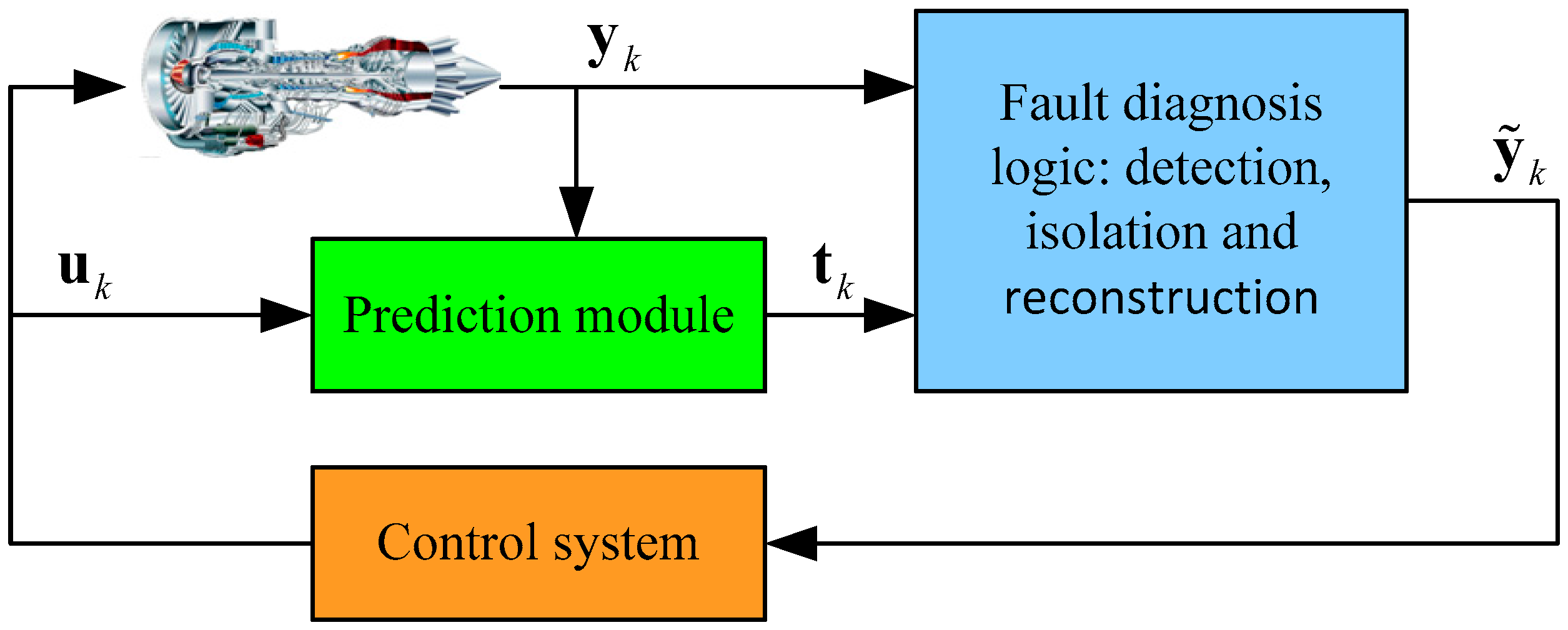
4. Sensor Fault Diagnosis for Aero Engines

As sensors have shortcomings of easy fault, FDI of a sensor system plays a very important part in ensuring the reliability of an aero engine control system. If the failure of sensors takes place, the safety of the aero engine would be seriously affected. Accurate sensor fault diagnosis with fast response is essential to enhance the reliability and safety of aero engines.

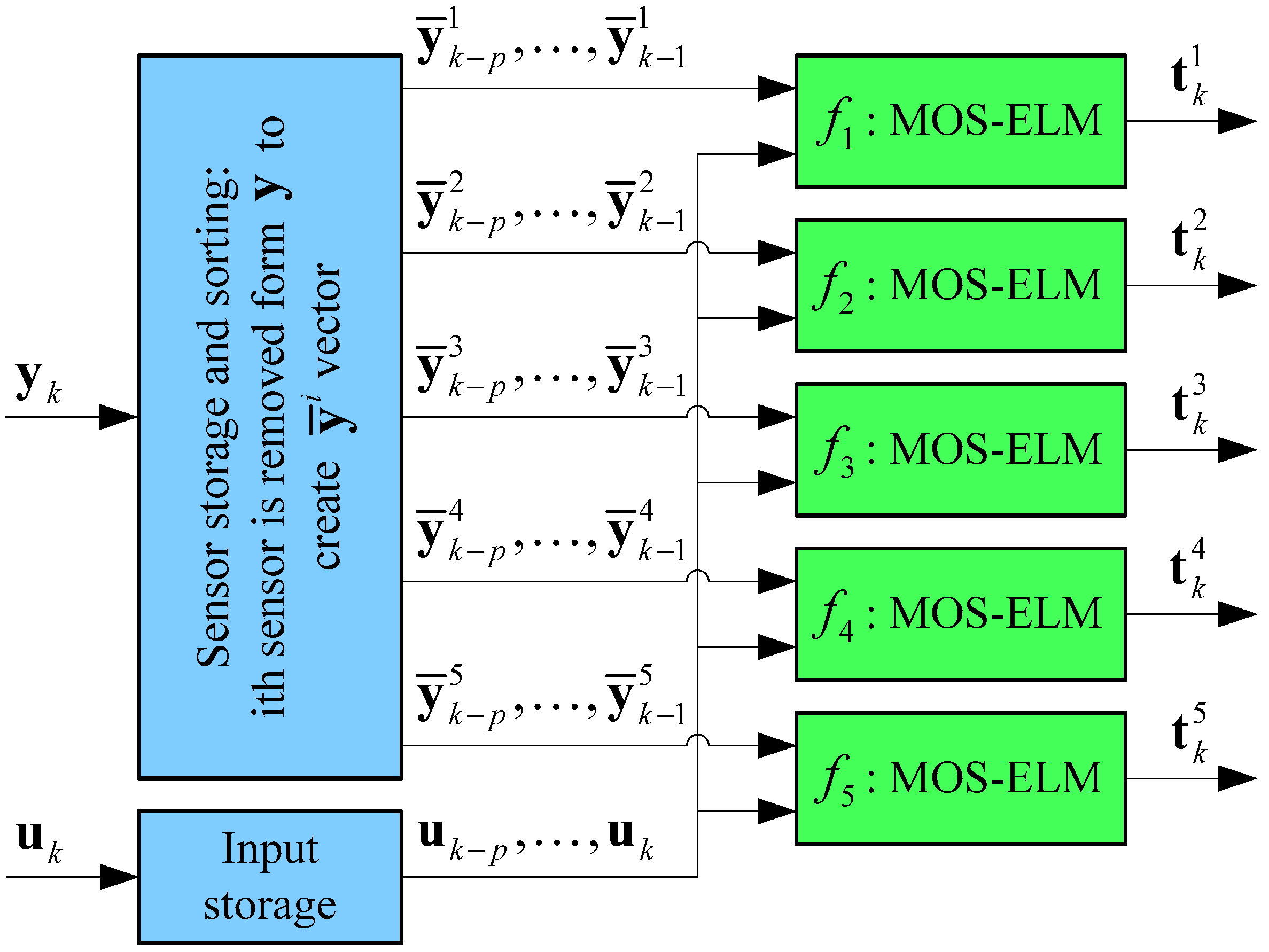
4.1. Diagnosis Method

Figure 1 illustrates the structure of the fault diagnosis and reconstruction system composed of the prediction module and fault diagnosis logic. The vector of measurements $y_k={\left[N_L,N_H,T_{22},P_{22},T_3\right]}_k^T$ consists of the low pressure rotor speed $N_L$, the high pressure rotor speed $N_H$, the fan discharge temperature $T_{22}$, the fan discharge pressure $P_{22}$, and the compressor discharge temperature $T_3$. The input vector $u_k={\left[W_{fb},A_8\right]}_k^T$ is composed of the fuel flow $W_{fb}$ and the area of nozzle throat area $A_8$ [34]. And $t_k$ denotes the prediction of the measurement vector $y_k$.

Figure 2 illustrates the prediction module of the fault diagnosis system according to the proposed MOS-ELM algorithm. Each measurement is predicted by an independent MOS-ELM respectively and is able to be mathematically expressed as:

$$\begin{array}{l}{t}_k^i=f_i\left(x_k\right),i=1,2,\dots ,5\\ x_k={\left[{{\overline{y}}_{k-p}^i}^T,\dots ,{{\overline{y}}_{k-1}^i}^T,u_{k-p}^T,\dots ,u_k^T\right]}^T\end{array}$$

(29)

where $t_k^i$ denotes the i-th element of $t_k$, $f_i(\cdot )$ represents the i-th MOS-ELM, ${\overline{y}}_{k-p}^i$ is created through removing i-th measurement $y_{k-p}^i$ form $y_{k-p}$, and $p$ denotes the embedding dimension for the prediction process.

The prediction of the measurement $t_k$ is used as an analytical channel for the diagnosis logic in Figure 1. If the discrepancy among the analytical channel $t_k$ and the measured channel $y_k$ exceeds a tolerance level, the fault diagnosis logic is able to determine the cause of the difference. For each measured parameter, the sensor fault indicator is introduced as the comparison of the analytical channel against the measured channel, and it is defined as follows:

$$r_k^i=\left|t_k^i-y_k^i\right|$$

(30)

where the analytical residual $r_k^i$ is the absolute difference between $t_k^i$ and $y_k^i$. Two typical kinds of sensor faults, drift fault and bias fault, are considered in this paper, and the thresholds for drift fault and bias fault are defined as $DC$ and $FC$ respectively. The analytical residual computed for each sensor is compared against the thresholds $DC$ and $FC$, and the detection logic can determine the fault level. If an analytical residual exceeds the bias fault threshold, it implies the existence of a bias fault. If an analytical residual exceeds the drift threshold and does not exceed the drift fault, it implies the existence of a drift fault.

If the drift fault or bias fault occurs, a correction strategy is applied to reconstruct the measurement and isolate the fault sensor. The correction trick is able to be described as the following equation:

$${\tilde{y}}_k^i=y_k^i+\left(t_k^i-y_k^i\right){\left(\min \left(1,\frac{r_k^i-DC}{FC-DC}\right)\right)}^{1/m}$$

(31)

where ${\tilde{y}}_k^i$ denotes the i-th reconstruction value of $y_k$ and $m>1$ is a correction factor. If the bias fault is detected, the measured value $y_k^i$ does not contain any effective information. Then the reconstruction value ${\tilde{y}}_k^i$ is completely determined by the prediction value $t_k^i$, and the fault measured value $y_k^i$ is isolated. In addition, if the drift fault is detected, we use the above correction strategy to properly utilize the information of the measurement and the prediction.

4.2. Diagnosis System for $N_L$ Sensor

In this subsection, we use a double-shaft turbofan component level model to be the research object and the measurement noise considered here is Gaussian with the standard deviation being 0.30% [35]. At $H=0\mathrm{km}$ and $Ma=0$, the acceleration and deceleration of an aero engine is simulated with the throttle lever angle in the interval ${30}^{\circ }–{70}^{\circ }$. Because the main dynamic characteristics of the aero engine can be considered to be a second-order element, the embedding dimension is set as $p=2$ [36]. In order to avoid affecting the weight in the diagnosis system, the measurements acquired from sensors are normalized into $\left[-1,1\right]$. The thresholds $DC$ and $FC$ are determined according to the compromise between false alarm rate and corrected detection rate. We select the thresholds from the following domain:

$$\begin{array}{l}DC\in \{x|x=0.013+0.0005k,k=1,2,3,\cdots ,8\}\\ FC\in \{x|x=0.023+0.0005k,k=1,2,3,\cdots ,8\}\end{array}$$

(32)

The best combination of $DC$ and $FC$ is selected manually considering the false alarm rate and corrected detection rate. For the OS-ELM case, the thresholds are selected as $DC=0.0145$ and $FC=0.0255$; and for the MOS-ELM case, the thresholds are selected as $DC=0.0140$ and $FC=0.0245$; and the correction factor is set as $m=2$. The magnitude of bias fault and drift simulated in this section is 3% and 0%–4%, respectively.

The diagnosis results based on OS-ELM and MOS-ELM algorithms for the $N_L$ sensor are illustrated in Figure 3 and Figure 4, respectively. The fault level of Figure 3b and Figure 4b is defined as follows: 0, no fault; 1, drift fault; 2, bias fault. The drift fault takes place during the interval $5–9\mathrm{s}$, and the bias fault comes up during the interval $34–38\mathrm{s}$. We can easily find that the reconstruction value by MOS-ELM is more accurate than that by OS-ELM, and the lower accuracy of OS-ELM tends to lead to a false alarm. With the prediction value being the analytical redundancy, the reconstruction value ${\tilde{y}}_k^i$ can effectively approximate the real value, ensuring the approximate validity of sensor signals even if the bias or drift fault happens. Hence, the right commands are able to be produced in accordance with the control law, and then the reliability and safety of aero engines is enhanced. Figure 5 illustrates the prediction bias of $N_L$ sensor by OS-ELM and MOS-ELM. It is obvious that MOS-ELM tends to generate more accurate predicted bias than OS-ELM, owing to handling the timeliness properly.

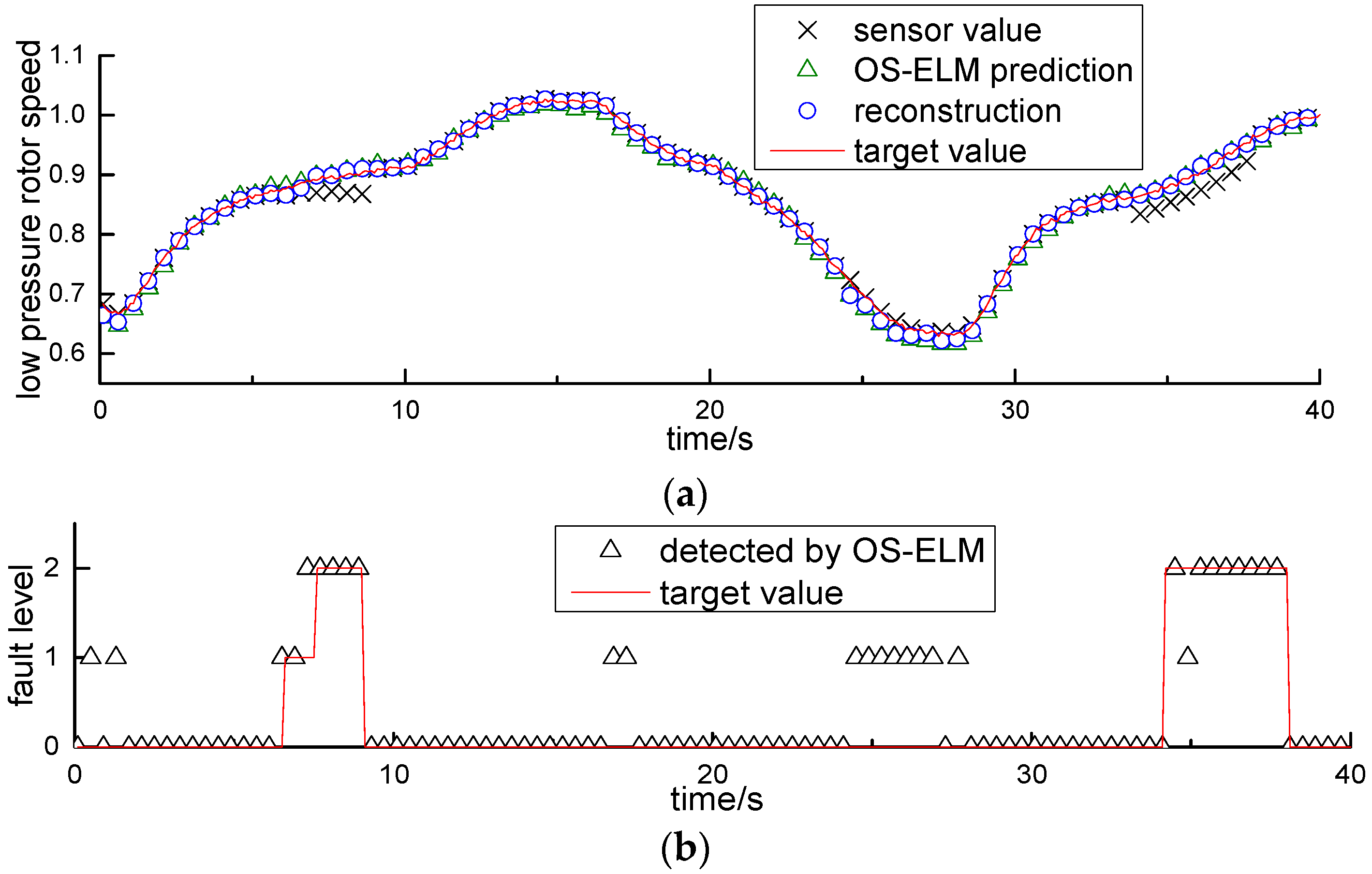
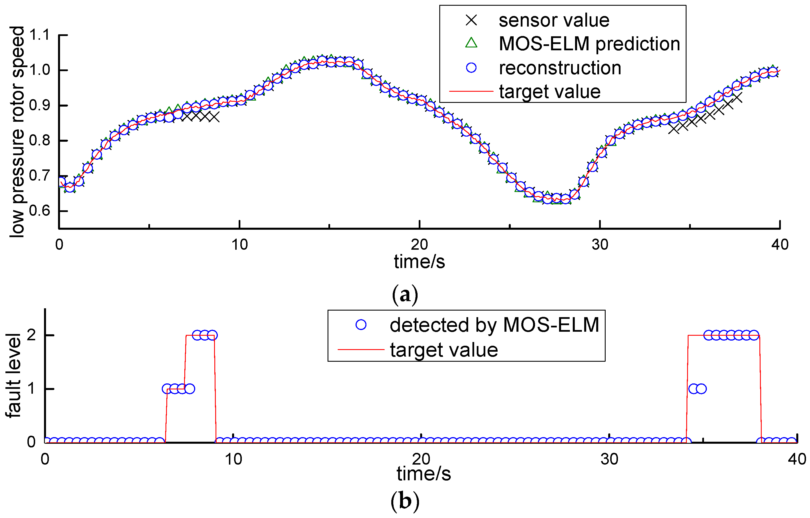
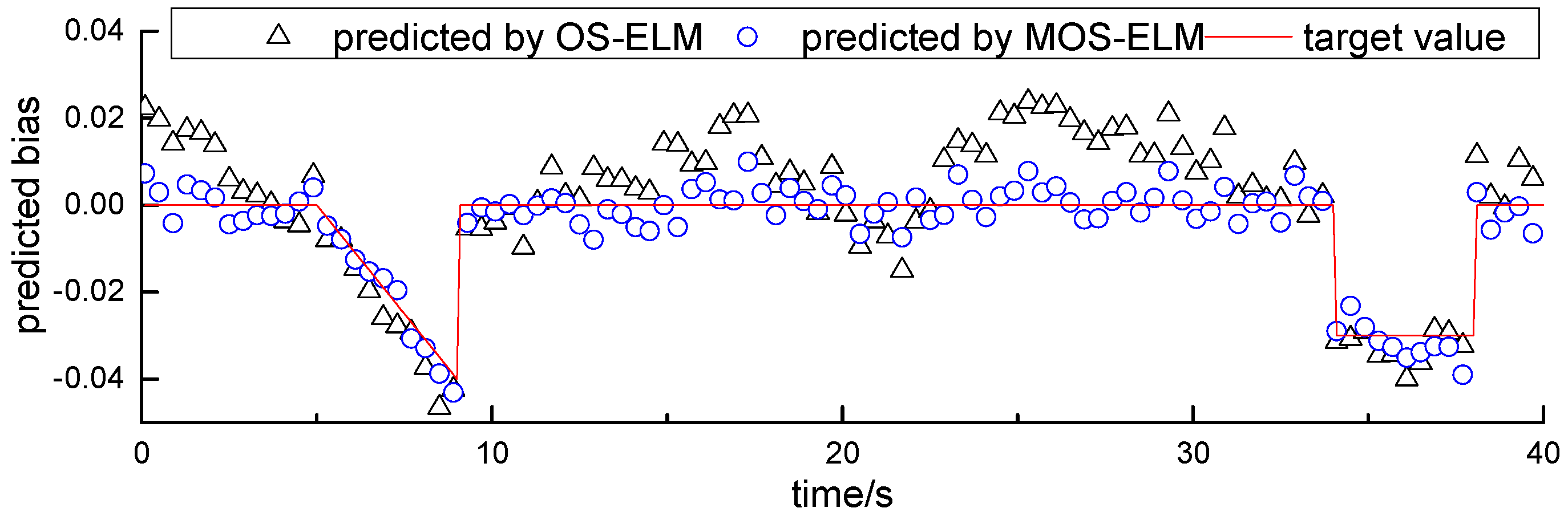
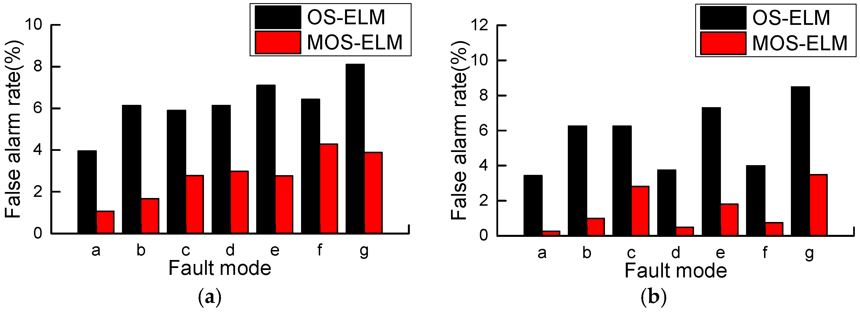
4.3. Statistical Performance for Different Fault Mode

Five kinds of single fault modes, $\left\{N_L\right\}$, $\left\{N_H\right\}$, $\left\{T_{22}\right\}$, $\left\{P_{22}\right\}$ and $\left\{T_3\right\}$, are considered in this subsection. The single fault mode $\left\{N_L\right\}$ denotes that $N_L$ breaks down alone, and the other four single fault modes follow suit. In addition, the case that more than one sensor are likely to break down at the same time is not overlooked. Two kinds of dual fault modes, $\left\{N_L,P_{22}\right\}$ and $\left\{N_H,T_3\right\}$, are considered here. The dual fault mode $\left\{N_L,P_{22}\right\}$ denotes that $N_L$ and $P_{22}$ break down at the same time, and $\left\{N_H,T_3\right\}$ represents that $N_H$ and $T_3$ break down simultaneously. For the purpose of obtaining robust statistical results, 20 different trials are carried out for each instance. Furthermore, in order to measure the learning performance, the root-mean-square error (RMSE) is defined as follows [37]:

$$\mathrm{RMSE}=\sqrt{\frac{{\displaystyle \sum _{i=1}^5{\displaystyle \sum _{k=1}^{\#\mathrm{Testing}}{\left(t_k^i-y_k^i\right)}^2}}}{\#\mathrm{Testing}\times 5}}$$

(33)

where #Testing denotes the testing samples number. In general, a smaller RMSE implies a better predicting accuracy for a learning algorithm. The average prediction RMSE for drift sensor fault and bias sensor fault is given in

Table 2. Comparison of prediction RMSE via OS-ELM and MOS-ELM.

Fault Mode	Algorithms	Drift Fault			Bias Fault
		RMSE	SD	Training Time (s)	RMSE	SD	Training Time (s)
$\left\{N_L\right\}$	OS-ELM	0.0293	0.0001	3.35	0.0284	0.0007	3.33
	MOS-ELM	0.0183	0.0008	3.32	0.0177	0.0010	3.27
$\left\{N_H\right\}$	OS-ELM	0.0508	0.0067	3.34	0.0558	0.0078	3.28
	MOS-ELM	0.0221	0.0032	3.31	0.0261	0.0056	3.27
$\left\{T_{22}\right\}$	OS-ELM	0.0432	0.0029	3.35	0.0456	0.0042	3.27
	MOS-ELM	0.0267	0.0033	3.32	0.0259	0.0027	3.32
$\left\{P_{22}\right\}$	OS-ELM	0.0405	0.0041	3.35	0.0315	0.0016	3.30
	MOS-ELM	0.0347	0.0070	3.34	0.0217	0.0019	3.27
$\left\{T_3\right\}$	OS-ELM	0.0471	0.0072	3.29	0.0464	0.0049	3.27
	MOS-ELM	0.0293	0.0042	3.36	0.0271	0.0045	3.31
$\left\{N_L,P_{22}\right\}$	OS-ELM	0.0384	0.0029	3.33	0.0319	0.0014	3.31
	MOS-ELM	0.0367	0.0046	3.32	0.0239	0.0020	3.32
$\left\{N_H,T_3\right\}$	OS-ELM	0.0696	0.0114	3.33	0.0800	0.0126	3.38
	MOS-ELM	0.0335	0.0063	3.36	0.0347	0.0050	3.30

Notes: RMSE: the root-mean-square-error; SD: standard deviation.

. It is obvious that the proposed MOS-ELM has lower prediction RMSE and superior generalization performance than OS-ELM in sensor fault diagnosis for aero engines, in both bias fault and drift fault cases, which can be attributed to properly tackling the timeliness of the sensor fault diagnosis system. Just as is derived by theory, the proposed MOS-ELM has no advantage in the aspect of the training time. For each instance, the training time for five learning machines is less than 4 s through the proposed MOS-ELM algorithm or OS-ELM algorithm, which corresponds to 40 s simulation duration. Thus, the real-time performance demand for an aero engine control system is completely met.

In addition, in order to measure the performance of the sensor fault diagnosis system, two performance indexes—the correct detection rate and the false alarm rate—is considered here. The average correct detection rate for drift sensor fault and bias sensor fault is given in

Table 3. Comparison of correct detection rate via OS-ELM and MOS-ELM.

Fault Mode	Algorithms	Drift Fault		Bias Fault
		CDR (%)	SD (%)	CDR (%)	SD (%)
$\left\{N_L\right\}$	OS-ELM	78.64	8.31	77.15	9.48
	MOS-ELM	90.31	5.04	96.13	2.42
$\left\{N_H\right\}$	OS-ELM	97.80	0.89	98.35	0.99
	MOS-ELM	97.23	0.95	99.48	0.47
$\left\{T_{22}\right\}$	OS-ELM	96.12	1.77	97.35	1.3
	MOS-ELM	99	0.83	99.48	0.41
$\left\{P_{22}\right\}$	OS-ELM	92.24	2.81	79.78	7.74
	MOS-ELM	93.5	1.65	95.55	2
$\left\{T_3\right\}$	OS-ELM	96.96	1.75	98.13	0.99
	MOS-ELM	96.92	1.3	99.45	0.46
$\left\{N_L,P_{22}\right\}$	OS-ELM	-	-	-	-
	MOS-ELM	98.94	3.68	99.63	1.3
$\left\{N_H,T_3\right\}$	OS-ELM	100	0	100	0
	MOS-ELM	99.94	0.14	99.84	0.73

Note: CDR: correct detection rate.

. Figure 6a,b illustrates the false alarm rate for drift sensor fault and bias sensor fault respectively. As observed from Table 3 and Figure 6, we can easily find that the MOS-ELM algorithm has a higher corrected detection rate and lower false alarm rate than OS-ELM algorithm. As a result of the coupling among the different sensors, the dual fault mode $\left\{N_L,P_{22}\right\}$ cannot be detected by the OS-ELM algorithm, while it can be detected well by the MOS-ELM algorithm.

5. Conclusions

In many real online learning applications, the sequentially arrived data usually has the characteristic of timeliness. The OS-ELM trains the neural network chunk by chunk, but at the same time, it cannot deal with the timeliness of the data chunk. Based on the OS-ELM algorithm, we propose a novel algorithm, MOS-ELM, which introduces the concept of memory principle into OS-ELM to improve the learning process by declining the validity of the outdated data chunk which may mislead the subsequent learning process. Thus MOS-ELM is able to learn sequentially as does the OS-ELM algorithm, but at the same time deals with the timeliness of data chunk properly.

Compared with OS-ELM, simulations on benchmark databases exhibit that MOS-ELM performs better in generalization performance, stability, and prediction accuracy while the tested problems possess the characteristic of timeliness. On this basis, MOS-ELM is employed in detecting, isolating, and reconstructing the fault sensor signal of aero engines. The experiment results show that MOS-ELM has better predictability and generalization performance than OS-ELM in diagnosing a sensor fault. Furthermore, the feasibility and effectiveness of the MOS-ELM-based sensor fault diagnosis system imply that the diagnosis system is an approach with great promise for enhancing the reliability and safety of the aero engine control system.

References

1. Litt, J.S.; Simon, D.L.; Garg, S.; Guo, T.H.; Mercer, C.; Millar, R.; Behbahani, A.; Bajwa, A.; Jensen, D.T. A survey of intelligent control and health management technologies for aircraft propulsion systems. J. Aerosp. Comput. Inf. Commun. 2005, 1, 543–563. [Google Scholar] [CrossRef]
2. Jaw, L. Recent advancements in aircraft engine health management (EHM) technologies and recommendations for the next step. In Proceedings of the ASME Turbo Expo 2005: Power for Land, Sea and Air, Reno, NV, USA, 6–9 June 2005.
3. Patton, R.J.; Chen, J. Robust fault detection of jet engine sensor systems using eigenstructure assignment. J. Guid. Control Dyn. 1992, 15, 1491–1497. [Google Scholar] [CrossRef]
4. Hwang, I.; Kim, S.; Kim, Y.; Seah, C.E. A survey of fault detection, isolation, and reconfiguration methods. IEEE Trans. Control Syst. Technol. 2010, 18, 636–653. [Google Scholar] [CrossRef]
5. Chow, E.Y.; Willsky, A.S. Analytical redundancy and the design of robust failure detection systems. IEEE Trans. Autom. Control 1984, 29, 603–614. [Google Scholar] [CrossRef]
6. Willsky, A.S. A survey of design methods for failure detection in dynamic systems. Automatica 1976, 12, 601–611. [Google Scholar] [CrossRef]
7. Wallhagen, R.E.; Arpasi, D.J. Self-Teaching Digital-Computer Program for Fail-Operational Control of a Turbojet Engine in a Sea-Level Test Stand; Report No. NASA/TM-X-3043; National Aeronautics and Space Administration, Glenn Research Center: Washington, DC, USA, 1974.
8. Bras, S.; Rosa, P.; Silvestre, C.; Oliveira, P. Fault detection and isolation in inertial measurement units based on bounding sets. IEEE Trans. Autom. Control 2015, 60, 1933–1938. [Google Scholar] [CrossRef]
9. Lu, F.; Chen, Y.; Huang, J.Q.; Zhang, D.; Liu, N. An integrated nonlinear model-based approach to gas turbine engine sensor fault diagnostics. Proc. Inst. Mech. Eng. G J. Aerosp. 2014, 228, 2007–2021. [Google Scholar] [CrossRef]
10. Bahareh, P.; Meskin, N.; Khorasani, K. Sensor fault detection, isolation, and identification using multiple-model-based hybrid Kalman filter for gas turbine engines. IEEE Trans. Control Syst. Technol. 2016, 24, 1184–1190. [Google Scholar]
11. Escobar, R.F.; Astorga-Zaragoza, C.M.; Hernandez, J.A.; Juarez-Romero, D.; Garcia-Beltran, C.D. Sensor fault compensation via software sensors: Application in a heat pump’s helical evaporator. Chem. Eng. Res. Des. 2015, 93, 473–482. [Google Scholar] [CrossRef]
12. Mattern, D.L.; Jaw, L.C.; Guo, T.H.; Graham, R.; McCoy, W. Using neural networks for sensor validation. In Proceedings of the 35th AIAA/ASME/SAE/ASEE Joint Propulsion Conference, Cleveland, OH, USA, 12–15 July 1998.
13. Sadough-Vanini, Z.N.; Meskin, N.; Khorasani, K. Multiple-model sensor and components fault diagnosis in gas turbine engines using autoassociative neural networks. J. Eng. Gas Turbines Power 2014, 136, 76–82. [Google Scholar] [CrossRef]
14. Torella, G.; Torella, R. Probabilistic expert systems for the diagnostics and trouble-shooting of gas turbine apparatuses. In Proceedings of the 35th AIAA/ASME/SAE/ASEE Joint Propulsion Conference, Los Angeles, CA, USA, 20–24 June 1999.
15. Garg, S.; Schadow, K.; Horn, W.; Pfoertner, H.; Stiharu, I. Sensor and actuator needs for more intelligent gas turbine engines. In Proceedings of the GT2005 ASME Turbo Expo 2010: Power for Land, Sea and Air, Glasgow, UK, 14–18 June 2010.
16. Bahareh, P.; Meskin, N.; Khorasani, K. Sensor fault detection and isolation using multiple robust filters for linear systems with time-varying parameter uncertainty and error variance constraints. In Proceedings of the 2014 IEEE Multi-Conference on Systems and Control, Antibes, France, 8–10 October 2014.
17. Kobayashi, T.; Simon, D.L. Evaluation of an enhanced bank of Kalman filters for in-flight aircraft engine sensor fault diagnostics. J. Eng. Gas Turbines Power 2014, 127, 635–645. [Google Scholar]
18. Saravanakumar, R.; Manimozhi, M.; Kothari, D.P.; Tejenosh, M. Simulation of sensor fault diagnosis for wind turbine generators DFIG and PMSM using Kalman filter. Energy Procedia 2014, 54, 494–505. [Google Scholar] [CrossRef]
19. Sadough-Vanini, Z.N.; Khorasani, K.; Meskin, N. Fault detection and isolation of a dual spool gas turbine engine using dynamic neural networks and multiple model approach. Inf. Sci. 2014, 259, 234–251. [Google Scholar] [CrossRef]
20. Tayarani-Bathaie, S.S.; Khorasani, K. Fault detection and isolation of gas turbine engines using a bank of neural networks. J. Process Control 2015, 36, 22–41. [Google Scholar] [CrossRef]
21. Shah, B.; Sarvajith, M.; Sankar, B.; Vijayendranath, V. Fault identification, isolation, estimation of sensor measurement using auto associative neural network for aero-engine. In Proceedings of the National Conference on Condition Monitoring, Chennai, India, 12–13 December 2014.
22. Ogaji, S.O.T.; Singh, R.; Probert, S.D. Multiple-sensor fault-diagnoses for a 2-shaft stationary gas-turbine. Appl. Energy 2002, 71, 321–339. [Google Scholar] [CrossRef]
23. Xu, L.; Cai, T.; Deng, F. Sensor fault diagnosis based on least squares support vector machine online prediction. In Proceedings of the 2011 IEEE 5th International Conference on Robotics, Automation and Mechatronics (RAM), Qingdao, China, 17–19 September 2011.
24. Zhang, S.; Li, Y. Simulation research on FLS_SVM in sensor fault diagnosis. In Proceedings of the 2011 International Conference on Electronic & Mechanical Engineering and Information Technology, Harbin, China, 12–14 August 2011.
25. Huang, G.B.; Zhu, Q.Y.; Siew, C.K. Extreme learning machine: A new learning scheme of feedforward neural networks. In Proceedings of the International Joint Conference on Neural Networks (IJCNN), Budapest, Hungary, 25–29 July 2004.
26. Huang, G.B.; Chen, L.; Siew, C.K. Universal approximation using incremental constructive feedforward networks with random hidden nodes. IEEE Trans. Neural Netw. 2006, 17, 879–892. [Google Scholar] [CrossRef] [PubMed]
27. Huang, G.B.; Zhou, H.M.; Ding, X.J.; Zhang, R. Extreme learning machine for regression and multiclass classification. IEEE Trans. Syst. Man Cybern. B 2012, 42, 513–529. [Google Scholar] [CrossRef] [PubMed]
28. Liang, N.Y.; Huang, G.B.; Saratchandran, P.; Sundararajan, N. A fast and accurate online sequential learning algorithm for feedforward networks. IEEE Trans. Neural Netw. 2006, 17, 1411–1423. [Google Scholar] [CrossRef] [PubMed]
29. Wang, N.; Er, M.J.; Han, M. Parsimonious extreme learning machine using recursive orthogonal least squares. IEEE Trans. Neural Netw. Learn. 2014, 25, 1828–1841. [Google Scholar] [CrossRef] [PubMed]
30. Deng, C.Y. A generalization of the Sherman-Morrison-Woodbury formula. Appl. Math. Lett. 2011, 24, 1561–1564. [Google Scholar] [CrossRef]
31. EI-Sayed, A.M.; Salman, S.M.; Elabd, N.A. On a fractional-order delay Mackey-Glass equation. Adv. Differ. Equ. 2016, 2016, 1–11. [Google Scholar]
32. Berezowski, M.; Grabski, A. Chaotic and non-chaotic mixed oscillations in a logistic systems with delay. Chaos Solitons Fractals 2002, 14, 97–103. [Google Scholar] [CrossRef]
33. Sunspot Index and Long-Term Solar Observations. Available online: http://www.sidc.be/silso/DATA/SN_m_tot_V2.0.txt (accessed on 10 June 2016).
34. Lu, F.; Huang, J.Q.; Xing, Y.D. Fault Diagnostics for Turbo-Shaft Engine Sensors Based on a Simplified On-Board Model. Sensors 2012, 12, 11061–11076. [Google Scholar] [CrossRef] [PubMed]
35. Kobayashi, T.; Simon, D.; Litt, J.S. Application of a constant gain extended Kalman filter for in-flight estimation of aircraft engine performance parameters. In Proceedings of the GT2005 ASME Turbo Expo 2005: Power for Land, Sea and Air, Reno, NV, USA, 6–9 June 2005.
36. Zhou, J.; Liu, Y.; Zhang, T.H. Analytical redundancy design for aeroengine sensor fault diagnostics based on SROS-ELM. Math. Probl. Eng. 2016, 2016, 8153282. [Google Scholar] [CrossRef]
37. Azad, A.K.; Rasul, M.G.; Yusaf, T. Statistical diagnosis of the best weibull methods for wind power assessment for agricultural applications. Energies 2014, 7, 3056–3085. [Google Scholar] [CrossRef]
Figure 1. Structure of sensor fault diagnosis and reconstruction system for aero engines.
Energies 10 00039 g001
Figure 2. Diagram of the prediction module of the fault diagnosis system according to proposed online sequential extreme learning machine with memory principle (MOS-ELM) algorithm.
Energies 10 00039 g002
Figure 3. (a) Reconstruction of N L sensor by OS-ELM; (b) Detected fault level of N L sensor by OS-ELM.
Energies 10 00039 g003
Figure 4. (a) Reconstruction of N L sensor by MOS-ELM; (b) Detected fault level of N L sensor by MOS-ELM.
Energies 10 00039 g004
Figure 5. Predicted bias of N L sensor by OS-ELM and MOS-ELM.
Energies 10 00039 g005
Figure 6. (a) Comparison of false alarm rate for drift fault; (b) Comparison of false alarm rate for bias fault. Note: the fault mode codes a , b , c , d , e , f , g correspond to { N L } , { N H } , { T 22 } , { P 22 } , { T 3 } , { N L , P 22 } and { N H , T 3 } , respectively.
Energies 10 00039 g006