Energy Rebound as a Potential Threat to a Low-Carbon Future: Findings from a New Exergy-Based National-Level Rebound Approach

Abstract

150 years ago, Stanley Jevons introduced the concept of energy rebound: that anticipated energy efficiency savings may be “taken back” by behavioural responses. This is an important issue today because, if energy rebound is significant, this would hamper the effectiveness of energy efficiency policies aimed at reducing energy use and associated carbon emissions. However, empirical studies which estimate national energy rebound are rare and, perhaps as a result, rebound is largely ignored in energy-economy models and associated policy. A significant difficulty lies in the components of energy rebound assessed in empirical studies: most examine direct and indirect rebound in the static economy, excluding potentially significant rebound of the longer term structural response of the national economy. In response, we develop a novel exergy-based approach to estimate national energy rebound for the UK and US (1980–2010) and China (1981–2010). Exergy—as “available energy”—allows a consistent, thermodynamic-based metric for national-level energy efficiency. We find large energy rebound in China, suggesting that improvements in China’s energy efficiency may be associated with increased energy consumption (“backfire”). Conversely, we find much lower (partial) energy rebound for the case of the UK and US. These findings support the hypothesis that producer-sided economies (such as China) may exhibit large energy rebound, reducing the effectiveness of energy efficiency, unless other policy measures (e.g., carbon taxes) are implemented. It also raises the prospect we need to deploy renewable energy sources faster than currently planned, if (due to rebound) energy efficiency policies cannot deliver the scale of energy reduction envisaged to meet climate targets.

1. Introduction: A Low Carbon Future—Under Threat from Energy Rebound

1.1. Concepts: Energy Efficiency and Energy Rebound

Reducing energy-related CO₂ emissions is a key component of energy policies designed to meet climate targets—given burning of fossil fuels accounts for around 80% [1] of global greenhouse gas (GHG) emissions. As illustrated in Figure 1, the path to a low carbon future is envisaged via two key policy-supported measures: the introduction of zero/low carbon energy sources [2], and the deployment of energy efficiency technologies to reduce energy use [3]. Efficiency-induced decoupling of global energy use from economic output (GDP) would mark a significant departure from observed history where energy-GDP have been tightly linked [4], in which case the feasibility and realism of emissions reduction strategies typical of Figure 1 is brought into question. Meanwhile, whilst authors including Alcott [5] advocate a strategy of sufficiency—by capping the production (or consumption) of products and services—the 5% CO₂ abatement from demand measures in Figure 1 suggests this has little envisaged role at present. This may reflect a simple truth: that reducing energy demand in the face of rising affluence is a hard task [6].

However, “energy rebound” is a potential threat to the success of energy efficiency technologies to reduce energy use at the scale envisaged. This occurs when “energy-saving innovations induce an increase in energy consumption that offsets the technology-derived saving” [8] (p. 40). Energy rebound is not a new concept: it is now more than 150 years since William Stanley Jevons in his book “The Coal Question” [9] made the counterintuitive claim that the introduction of energy efficient technologies to the Scottish coal mining industry had led to increases rather than reductions in energy consumption.

To understand rebound further, we now outline the components of energy rebound. At a national level, energy rebound is comprised of microeconomic and macroeconomic mechanisms, as shown in

Table 1. Typical components of energy rebound, based on Greening et al. [12] and Jenkins et al. [13].

Component of Energy Rebound	Origin/Mechanism
Microeconomic rebound: these rebound mechanisms occur within the static economy, based on responses to the reduction in implicit price of an energy service.	Direct rebound: describes the direct response to the energy efficiency improvement.	Jenkins et al. [13] split into two sub-classes: Income/output effects: This is the increasing demand for that energy service by producers to expand their output (“an output effect”) or consumers (an “income effect”). Substitution effects: this captures the substitution of that energy service for the other goods or services (consumers) or inputs to production (producers).
	Indirect rebound: this captures the indirect effects of direct energy rebound.	Jenkins et al. [13] split into two sub-classes: Embodied energy effects: The energy “embodied” in the efficiency improvements themselves will offset some portion of the energy savings achieved. Re-spending and re-investment effects: If consumers and firms see net cost savings from energy efficiency improvements, this may increase consumer expenditures or investments in production—increasing demand for goods, services, and factors of production, which in turn require energy to produce and support.
Macroeconomic rebound	These mechanisms originate from the dynamic response of the economy to reach a stable equilibrium (between supply and demand for goods and energy services).	Greening et al. [12] split these into two sub-classes: Economy-wide effects: shorter-term induced changes in prices and quantities of goods/services throughout the economy, to reach a new, stable equilibrium. Transformational effects: these stem from longer term change to consumers' preferences, social institutions, and rearrangement of the organization of production.

.

Following Saunders [10] and Wei [11], we formally define energy rebound, $Re$, by Equation (1), where ${\mathsf{\eta }}_{\mathsf{\tau }}^E$ is the elasticity of energy use $\left(E\right)$ with respect to energy efficiency gain ($\mathsf{\tau }$):

$$Re=\left(1+{\mathsf{\eta }}_{\mathsf{\tau }}^E\right)\times 100=\left(1+\frac{Changeinenergyuse(\%)}{energyefficiencygain(\%)}\right)\times 100$$

(1)

Behavioural responses to the adoption of energy efficient technologies affect the level of energy savings actually delivered, leading to five possible states of energy rebound as shown in

Table 2. States of energy rebound (adapted from Saunders [10]) (p. 2197).

State of Energy Rebound, $\mathit{R}\mathit{e}$ (%)	∆E, Change in Energy Use from 1% Efficiency Gain
Super-conservation ($Re$ < 0%)	∆E < −1%
Zero ($Re$ = 0%)	∆E = −1%
Partial (0% < $Re$ < 100%)	−1% < ∆E < 0%
Full ($Re$ = 100%)	∆E = 0%
Backfire ($Re$ > 100%)	∆E > 0%

. For example, a 1% efficiency gain and 0.5% reduction in energy use would yield $Re$ = 50%, which is a case of partial rebound. Jevons’ paradox [9] in the 1800s referred to the case of backfire ($Re$ > 100%).

Referring to Figure 1, the potentially significant importance of energy rebound to a low-carbon future is now revealed. On one hand, if national energy rebound is small (say 0%–10%), energy efficiency policies will be largely unaffected by rebound, and will translate into effective emissions reductions. On the other hand, if energy rebound is large ($Re$ > 50%), failure to account for rebound effects will lead to an significant overestimate of the effectiveness of energy efficiency policies—with serious implications for meeting emission reduction targets.

1.2. The Issue: More Empirical National Energy Rebound Studies Are Required

The Intergovernmental Panel on Climate Change (IPCC) acknowledge the potential importance of rebound to energy policy, stating “by considering the size of the rebound effect, a more-realistic calculation of energy-efficiency measures can be achieved providing a clearer understanding of their contribution to climate policy” [14] (p. 391). It is then perhaps surprising that energy rebound appears largely ignored by policymakers—Maxwell et al.’s [15] study of rebound for the European Commission highlighted the UK government’s Department of Energy and Climate Change (DECC) as the “only case example identified where the direct rebound effect is now recognised and factored into energy policy development guidance and tools”. Similarly, Font Vivanco et al. [16] find only two other examples—in Ireland and the USA—of policy including rebound effects: For the most part though, rebound is absent from energy policy: for example there is no mention of rebound in the UK’s Energy Bill [17] or the European Commission’s Energy Directive [3]. Thus whilst policymakers are aware of rebound as a topic [15], the current empirical literature has not had sufficient impact to penetrate energy policy [16,18,19,20]. This situation arguably contradicts the “Precautionary Principle”, which “emphasizes anticipation and prevention of future risks, even in the absence of full scientific certainty about the impacts of climate change” [14] (p. 1009). Aligning actions to the Precautionary Principle would mean nations conservatively accounting for energy rebound in their energy efficiency policies—given the urgency of required climate mitigation.

The nature of current empirical rebound literature—which serves as an evidence-base to inform energy policy—provides a potential explanation. On one hand, there is a growing range of empirical studies—for example refer to review studies by Sorrell and colleagues [21,22,23,24,25] and Jenkins et al. [13]. On the other hand, the empirical literature mainly focusses on part of the whole national energy rebound—in particular, (referring to Table 1) microeconomic studies of consumer-sided energy rebound. Such empirical studies range from direct rebound effects in personal transport [26,27] to broader consumer/household studies of direct-plus-indirect rebound effects [28,29]. The IPCC [1] concluded the majority of (empirical) household studies suggested (direct and indirect) rebound in developed countries may typically erode 20%–45% of potential energy savings.

The narrower focus (of most empirical studies) on consumer-sided direct/indirect rebound is therefore only part of the picture for national energy rebound. It misses producer-sided (direct and indirect) rebound, which studies suggest may give higher energy rebound [30,31,32], and also excludes the macroeconomic rebound effects from the long term structural response of the economy. As a result, empirical studies of national energy rebound—which consider all components in Table 1—are rare. By considering only part of national energy rebound, studies may be underplaying the true magnitude (and importance) of energy rebound—for example several recent studies [32,33,34,35,36] suggest national energy rebound may over 50%, and in some cases over 100%.

If national energy rebound—i.e., including all components of Table 1—is indeed significant, then this would have knock-on implications for the design of energy and climate policy. Therefore, more estimates of national energy rebound are required to strengthen the evidence base to better inform both energy-economy modelling [37,38,39] and policy.

1.3. The Response: An Exergy-Based Approach to Estimate National Energy Rebound

Our novel approach to estimating national energy rebound is centred on the inclusion of exergy efficiency as a national energy efficiency metric. Exergy, a term introduced in 1956 by Rant [40], was defined simply by Reistad [41] as the thermodynamic measure of “available energy”, meaning it is the “usable” part of energy—i.e., available to perform physical work. Largely in response to the energy crises of the 1970s, several exergy-based studies of energy consumption were completed [41,42,43,44], having considerable synergy with the parallel field of thermo-economics developed largely by Georgescu-Roegen [45,46,47] at the same time. As energy prices fell, interest in national-level exergy analysis waned, until a resurgence of interest in the 2000’s led by Ayres and Warr [48,49,50].

To illustrate how energy and exergy are different, let us consider the thermal energy content of the water molecules in a room full of air, and a 12 V car battery. Both “systems” have the same (first law) thermal energy content (in Joules), but only the 12 V battery has energy in concentrated, usable form (i.e., exergy) from which we can extract physical work. Thus exergy is a measure of thermodynamic energy quality, defined more formally by Ayres and Warr [50] (p. 186) as “the maximum work that a subsystem can do as it approaches thermodynamic equilibrium (reversibly) with its surroundings”. Unlike energy, which (in first law terms) can be neither created nor destroyed, some exergy is necessarily destroyed in all real-world conversion processes. As energy flows through a conversion chain, the usable part reduces in size until it is fully dissipated (the last measurable stage being at the point of useful exergy) in exchange for energy services, as illustrated in Figure 2.

By considering exergy consumption across all energy end use categories (i.e., heat, electrical end use, mechanical drive and muscle work), exergy accounts from primary-to-useful stages can be constructed for entire countries [50,51,52], as illustrated in Figure 3.

The aim of such aggregate, national exergy studies to date [50,51,54,55,56] has been to study trends over time of aggregate exergy efficiency (as defined in Equation (2)) and useful exergy, or explore the relationship between energy consumption and economic growth.

$$Exergyefficiency,\mathsf{\tau }=\frac{output\left(useful\right)exergy}{inputexergy}$$

(2)

To date, these exergy-based studies have not been applied to the area of energy rebound. This is the research gap we seek to explore. In response, we adopt aggregate national exergy efficiency ($\mathsf{\tau }$) as our metric for energy efficiency in Equation (1) and use it to estimate national energy rebound (i.e., considering all-components of Table 1). In doing so, we address Patterson’s observation that such thermodynamic metrics are not in use, despite appearing “the most natural or obvious way to measure energy efficiency” [57]. (p. 378) Referring to Figure 3—we estimate energy rebound at the primary stage (i.e., the level of extracted energy), since this is the relevant point for climate (emissions) policy. We estimate national energy rebound for three countries (US, UK, China), using two different methods based on aggregate production functions (APFs). Whilst other studies such as Zhang and Lin [33] consider multiple methods for a single country, and Malpede and Verdolini [58] consider multiple countries with a single method, this is believed to be the first combined multi-country multi-method empirical study. Our approach is intentional, to allow comparisons, and expand the rebound evidence base.

Finally, a note on boundaries and terminology, which are designed to match the aggregate national level of climate (emissions) policy. First, the estimates are strictly those of primary exergy rebound, since the efficiency metric (τ) records the efficiency of energy conversion from primary-to-useful stages, measured in exergy (as available energy) terms. However, as primary exergy-to-energy ratios are 1.04–1.08 for fossil fuels [59,60], aggregate primary energy and primary exergy values (in Joules) are close [53] in fossil-dominated economies. This means primary “exergy” or “energy” rebound values will be also very close. Therefore, to link to existing rebound literature, we use the term “energy rebound” from this point. Second, our study uses a territorial boundary of national energy use (and thus rebound), thereby accounting for the energy used within the geographic country boundaries—as opposed to a consumption-based assessment which would include trade flows of products with embodied energy. Third, our use of “aggregate” in “aggregate” production functions means at the national level, rather than at a more granular (e.g., industry sector or firm-level) scale.

2. Methods and Data

2.1. Step 1: Selecting the Aggregate Production Function

APFs are the basis for our estimation of national energy rebound. They seek to explain economic “production” or “output” (typically measured at the national scale as GDP) through a series of input “factors of production”. Lloyd [61] and Mishra [62] provide excellent papers on the history of APFs. Today, the two most common APFs in use [63] are the Cobb-Douglas (C-D) function and the constant elasticity of substitution (CES) function. APFs are widely used in the fields of growth accounting [64,65,66], macroeconomic models [67,68,69,70,71] and importantly for us—the estimation of energy rebound [11,38,72,73]. Therefore, APFs as the starting point for our exergy-based method makes sense.

An example of the C-D function is given in Equation (3), where economic output $(Y_t)$ is related to capital ($K_t$) and labour $(L_t)$ inputs:

$$Y_t=\mathsf{\theta }{e}^{\mathsf{\lambda }t}{K}_t^{\mathsf{\alpha }}{L}_t^{\mathsf{\beta }}$$

(3)

where α, β are the elasticities of output ($Y_t$) with respect to capital and labour respectively; θ is scale parameter (for base-year); $e^{\mathsf{\lambda }t}$ is the Solow residual—the share of output not explained by $K_t$ and $L_t$; $t$ is time relative to the base year; and λ is exogenous growth, equal to the rate of change in the Solow residual.

To select our APF, we next make three choices. The first (and most obvious) is to add energy (E) as a third factor of production, in order to explore and estimate energy rebound. The second is to use the CES function, which allows a broader range of possible values for the unknown parameters compared to the C-D function, including non-unity elasticity of substitution between inputs. The third choice is to “nest” the inputs, since as Sorrell [74] notes, the alternative non-nested CES function—where all elasticities of substitution are equal—provides a very restricted (and unlikely) scenario. Our preference is for a two-level KL-E functional structure, where capital-labour are in an inner nest, and energy is in the outer nest. This matches the structure of the most common macroeconomic models used to inform climate policy [32,75], and as Saunders also reported [10] (p. 2199) KL-E is the most “rebound flexible” CES function structure—permitting all rebound states in Table 2 except the (unlikely) super-conservation scenario. It also matches the nesting structure of other recent empirical rebound studies [32,33].

The resulting KL-E CES function is shown in Equation (4):

$$Y_t=\mathsf{\theta }{e}^{\mathsf{\lambda }t}{[{\mathsf{\delta }}_1{\left[(\mathsf{\delta }{K}_t^{-{\mathsf{\rho }}_1}+\left(1-\mathsf{\delta }\right)L_t^{-{\mathsf{\rho }}_1}\right]}^{\mathsf{\rho }/{\mathsf{\rho }}_1}+\left(1-{\mathsf{\delta }}_1\right)E_t^{-\mathsf{\rho }}]}^{-\frac{1}{\mathsf{\rho }}}$$

(4)

where ρ, ρ₁ are substitution parameters which indicate the ease of substituting one input for another, and are used to calculate Hicks Elasticities of Substitution (HES) between capital and labour (via ${\mathsf{\sigma }}_1=1/\left(1+{\mathsf{\rho }}_1\right)$) and between capital-labour and energy (via $\mathsf{\sigma }=1/\left(1+\mathsf{\rho }\right)$); δ, ${\mathsf{\delta }}_1$ are output share parameters which specify the weight of contribution from each input (values between 0 and 1) to economic output (note that output share parameters are different from output elasticities, which measure the change in output from a change of a single input factor of production).

2.2. Step 2: Specifying and Estimating the Exergy-Based CES Function Parameters

2.2.1. The Exergy-Based CES Function

Our aim is to econometrically obtain fitted values for the unknown parameters of an exergy-based CES function, in order to use these parameter values in the derived rebound equations (Section 2.3). To do this, we need to define the exergy-based CES function. We start by adopting useful exergy (U) as the input energy factor of production, which translates Equation (4) to the exergy-based CES function given in Equation (5):

$$Y_t=\mathsf{\theta }{e}^{\mathsf{\lambda }t}{[{\mathsf{\delta }}_1{\left[(\mathsf{\delta }{K}_t^{-{\mathsf{\rho }}_1}+\left(1-\mathsf{\delta }\right)L_t^{-{\mathsf{\rho }}_1}\right]}^{\mathsf{\rho }/{\mathsf{\rho }}_1}+\left(1-{\mathsf{\delta }}_1\right)U_t^{-\mathsf{\rho }}]}^{-\frac{1}{\mathsf{\rho }}}$$

(5)

Including $U$ as the energy input has support in the wider economic literature—various researchers including Ayres and Warr [50,76] and Voudouris et al. [77] claim that useful exergy—not primary energy or final energy—provides the energy “input” which is most closely linked to economic growth.

Next, we normalise the inputs (K, L, E) and output (Y) to a starting (base) year, in line with recommendations by Temple [78] and Klump et al. [69]. This overcomes a key criticism of empirical APFs, that aggregate variables with differing units cannot be combined. Our input data is normalised to base years of 1980 (UK and US) and 1981 (China). By convention, the aggregate variables $\left(Y,K,L,U\right)$ become lower case ($y,k,l,u)$ when normalised, such that $y_t=Y_t/Y_0$; $k_t=K_t/K_0$; $l_t=L_t/L_0$; $u_t=U_t/U_0$; which modifies Equation (5) to become Equation (6), which is the final CES form econometrically fitted:

$$y_t=\mathsf{\theta }{e}^{\mathsf{\lambda }t}{[{\mathsf{\delta }}_1{\left[(\mathsf{\delta }{k}_t^{-{\mathsf{\rho }}_1}+\left(1-\mathsf{\delta }\right)l_t^{-{\mathsf{\rho }}_1}\right]}^{\mathsf{\rho }/{\mathsf{\rho }}_1}+\left(1-{\mathsf{\delta }}_1\right)u_t^{-\mathsf{\rho }}]}^{-\frac{1}{\mathsf{\rho }}}$$

(6)

2.2.2. Input Data

Now that the CES function (Equation) is obtained, we assemble input data (y, k, l, u) for each country, before econometrically estimating the six unknown parameters: $\mathsf{\theta },\mathsf{\lambda },\mathsf{\delta },{\mathsf{\delta }}_1,\mathsf{\rho },{\mathsf{\rho }}_1$. The factors of production and economic output (prior to normalisation) are annual time-series of Y, K, L, and U, for the UK (1980–2010), US (1980–2010), and China (1981–2010). The output measure (Y) is taken as aggregate GDP in 2005US$ constant prices from the Penn World Tables (PWT) 8.1 [79]. Capital, labour and energy data are all quality-adjusted, meaning they seek to better account for the productive effect of raw capital (stock), labour (workhours) and (primary) energy. Quality-adjusted inputs are now commonly used in growth accounting studies [80,81,82].

For labour, quality-adjusted total hours are obtained via human capital indices from Barro and Lee [83], multiplied by average workhours for the US and UK from PWT8.1 [79], and for China from Wu [84]. Quality-adjusted capital is taken as capital services: a measure of the flow of productive services from a capital asset. Capital service data for 1980–2010 was sourced for the UK [85] and the US [86,87]. For China, capital service data was obtained for 1981–2010 from Wu [88]. The limitations in the availability of capital services data constrains the time-period for the study. Previously calculated values of useful exergy (as quality-adjusted energy) for the UK, US and China are taken from Brockway et al. [53,89].

The normalised input datasets (y, k, l, u) are shown in Figure 4, Figure 5, Figure 6 and Figure 7:

2.2.3. Econometric Fitting of the CES Aggregate Production Function

Last, we obtain values for the six unknown parameters: $\mathsf{\theta },\mathsf{\lambda },\mathsf{\delta },{\mathsf{\delta }}_1,\mathsf{\rho },{\mathsf{\rho }}_1$, by econometrically fitting Equation (6) using a customised version of the iterative, non-linear technique developed by Henningsen and Henningsen [90,91]. Two steps are completed. First, we determine “base-fit” values for the six parameters by fitting to the historical data. Secondly, to provide an indication of the precision we can attach to values of the CES parameters (and later, overall rebound), we use a “bootstrapping” resampling technique on the CES equation to resample the residuals, following the detailed description in Heun et al. [92]. Whilst bootstrapping is becoming more commonly used in APF-based growth accounting studies [70,80,81], to our knowledge this is the first use in an empirical rebound study. We resample the residual values 1000 times and re-fit to obtain resample estimates of CES parameters. We report the 2.5% and 97.5% values (i.e., those of the 25th and 976th ranking in order of magnitude) to provide an indication of the precision with which the original parameter estimates are known.

2.3. Step 3: Derive Equations for Estimation of National Energy Rebound

With the function and the estimation process in place, we now present two approaches (which use the fitted CES parameter values) to estimate overall values for national energy rebound. Both methods have been previously used for the estimation of energy rebound [33,73,93,94,95] and so provide a suitable place to introduce new (exergy efficiency and useful exergy) datasets. Whilst being based on the parameters determined from the same econometrically fitted CES function, they adopt very different independent variables (and thus routes) for the estimation of rebound effects: the first adopts factor-neutral technical change (λ) whilst the second uses the exergy efficiency metric (ε). Further discussion of the two methods is given in Section 4.3.

2.3.1. Method 1: Ratio of Actual to Potential Energy Savings (AES/PES)

The method is based on estimating the ratio of actual energy savings (AES) to potential energy savings (PES), such that rebound is defined as Equation (7). Hence if AES equals PES, then Re = 0 (zero rebound), whilst if AES is zero, then Re = 1.0.

$$Re=1-\frac{\mathrm{Actual}\mathrm{Energy}\mathrm{Saved}\left(AES\right)}{\mathrm{Potential}\mathrm{Energy}\mathrm{Saved}\left(PES\right)}=\frac{\left(PES\right)-\left(AES\right)}{\left(PES\right)}$$

(7)

We follow the approach of Zhang and Lin [33] and Shao et al. [73], who completed empirical rebound studies by translating Equation (7) into a rebound equation which is based on the CES function parameters. Their logical derivation starts by finding an expression for the denominator (PES). Taking $Y_t$ as GDP in year t, and $E{I}_t$ as energy intensity ($E_t$/$Y_t$) in year t, the energy use in year t is thus $Y_t$ × $E{I}_t$, whilst in year t + 1 it is $Y_{t+1}$ × $E{I}_{t+1}$. However, if no energy efficiency gains occurred from year t to t + 1, energy intensity remains unaltered ($E{I}_t$), and the energy use in year t + 1 would be $Y_{t+1}$ × $E{I}_t$. Therefore, the PES term is given by Equation (8):

$$PES=(Y_{t+1}\times E{I}_t-Y_{t+1}\times E{I}_{t+1})=Y_{t+1}\times (E{I}_t-E{I}_{t+1})$$

(8)

The expression for the numerator is based on the central assumption that “take-back” of energy consumption (PES-AES) in year t + 1 is seen via ${\mathsf{\lambda }}_{t+1}$, i.e., exogenous (all-factor) technical progress. In other words, it assigns the rebound of energy (from energy efficiency) to exogenous growth λ, meaning if λ = 0 then there is no energy rebound. In aggregate energy terms, the rebound energy consumption (PES-AES) is given by the fraction of economic growth attributable to exogenous growth [${\mathsf{\lambda }}_{t+1}$ × ($Y_{t+1}-Y_t$)] multiplied by the energy intensity in year t + 1 ($E{I}_{t+1}$), as shown in Equation (9):

$$PES-AES=[{\mathsf{\lambda }}_{t+1}\times (Y_{t+1}-Y_t)]\times (E{I}_{t+1})$$

(9)

The resultant overall expression for energy rebound (from year t to t + 1) is given in Equation (10):

$$R{e}_{t+1}=\frac{{\mathsf{\lambda }}_{t+1}\left(Y_{t+1}-Y_t\right)\left(E{I}_{t+1}\right)}{Y_{t+1}\left(E{I}_t-E{I}_{t-1}\right)}$$

(10)

The input data sources are primary energy consumption ($E_t)$ from the IEA [96]: GDP $(Y_t$) from PWT8.1 [79]; and yearly values for the parameter ${\mathsf{\lambda }}_{t+1}$ from the econometric fitting of the CES function in Equation. The values obtained for $R{e}_{t+1}$ at each year (t + 1, t + 2, etc.) then enable the estimation of national energy rebound for the UK, US and China by taking the mean value of $R{e}_{t+1}$ from all the values obtained.

2.3.2. Method 2: Elasticity of Energy Use with Respect to Efficiency (EEE)

This method is based on deriving an expression for ${\mathsf{\eta }}_{\mathsf{\tau }}^E$ from the CES function, the elasticity of energy use (in our case primary exergy, E) with respect to exergy efficiency, $\mathsf{\tau }$. The expression for ${\mathsf{\eta }}_{\mathsf{\tau }}^E$ can then be inserted back into Equation (1) ($Re=(1+{\mathsf{\eta }}_{\mathsf{\tau }}^E)\times 100)$ which can then be evaluated to given an empirical estimate for national energy rebound.

To do this, we proceed in several stages. First, we insert $U_t={\mathsf{\tau }}_t{E}_t$ into Equation (5), where ${\mathsf{\tau }}_t$ is exergy efficiency and $E_t$ is primary exergy, yielding Equation (11):

$$Y_t=\mathsf{\theta }{e}^{\mathsf{\lambda }t}{[{\mathsf{\delta }}_1{\left[(\mathsf{\delta }{K}_t^{-{\mathsf{\rho }}_1}+\left(1-\mathsf{\delta }\right)L_t^{-{\mathsf{\rho }}_1}\right]}^{\mathsf{\rho }/{\mathsf{\rho }}_1}+\left(1-{\mathsf{\delta }}_1\right){\left({\mathsf{\tau }}_t{E}_t\right)}^{-\mathsf{\rho }}]}^{-\frac{1}{\mathsf{\rho }}}$$

(11)

There are close similarities with the APFs proposed for the estimation of aggregate energy rebound by Saunders [10] in Equation (12) and Wei [11] in Equation (13) which both combine $\mathsf{\tau }$ (as an engineering efficiency parameter) with final energy consumption. Fundamentally, this shares our assumption that it is the energy use at the end of energy conversion stages (in our case via useful exergy) that serves as the appropriate input to the production function, not primary energy.

$$Y={\left[a{(K^{\propto }{L}^{1-\propto })}^{\mathsf{\rho }}+b{\left(\mathsf{\tau }E\right)}^{\mathsf{\rho }}\right]}^{\frac{1}{\mathsf{\rho }}}$$

(12)

$$Y=\mathrm{f}\left(K^d,\mathsf{\tau }{E}^d\right)$$

(13)

Similarities aside, the CES function in Equation (11) has greater flexibility than Saunders’s use of the Hogan-Manne [97] CES function (where KL is a C-D function) and Wei’s C-D function. Our approach therefore provides a larger range of possible values for the fitted parameters, which is desirable to allow the best possible estimate of rebound.

Second, we derive an expression for ${\mathsf{\eta }}_{\mathsf{\tau }}^E$ based on the CES function. Saunders [10] previously derived such an expression based on the more restrictive Hogan-Manne CES function given in Equation (12). Thus, we must derive a new expression for ${\mathsf{\eta }}_{\mathsf{\tau }}^E$, since our APF is in the extended CES format of Equation (11). It follows a very similar process outlined by Saunders [10] for the CES (Solow) production function. A full derivation is given in the Supplementary Information, with the summary logic explained now.

To start we recap our aim: to assess how primary exergy use ($E)$ responds to changes in the energy efficiency gain parameter $\left(\mathsf{\tau }\right)$, as given in Equation (14):

$$Re=1+{\mathsf{\eta }}_{\mathsf{\tau }}^E=1+\frac{\mathsf{\tau }}{E}\frac{\partial E}{\partial \mathsf{\tau }}$$

(14)

We cannot obtain $\frac{\mathsf{\tau }}{E}\frac{\partial E}{\partial \mathsf{\tau }}$ directly from the CES function, so it is obtained indirectly via the Implicit Function Theorem. First we set up three implicit functions (i.e., of the form $g\left(x,y\right)=0$) using the production function itself and two first-order economic theory conditions, whereby energy and capital supply are adjusted in the long term such that the real price of energy ($\frac{\partial Y}{\partial E}$ = $\frac{p_E}{c}$) and capital ($\frac{\partial Y}{\partial K}$ = $\frac{p_K}{c}$) are fixed and equal to their marginal productivities. The implicit functions are thereby of the form shown in Equation (15):

$$\begin{gathered} {\mathsf{\psi }}_1=g\left(Y,f(K,L,\mathsf{\tau }E\right)=0 \\ {\mathsf{\psi }}_2=h\left(\frac{p_F}{c},\frac{\partial f(K,L,\mathsf{\tau }E}{\partial E}\right)=0 \\ {\mathsf{\psi }}_3=k\left(\frac{p_K}{c},\frac{\partial f(K,L,\mathsf{\tau }E}{\partial K}\right)=0 \end{gathered}$$

(15)

From the vector ($\mathsf{\Psi }=({\mathsf{\psi }}_1,{\mathsf{\psi }}_2,{\mathsf{\psi }}_3)$), a Jacobian matrix assembling their partial derivatives is then constructed in the form $J=\left[\frac{\partial {\mathsf{\psi }}_i(Y_0,E_0,{\mathsf{\tau }}_0)}{\partial X_j}\right]$, where $X_j=Y,E,K$. With the Jacobian matrix now in place, we apply the Implicit Function Theorem, which allows us to implicitly (i.e., rather than explicitly) derive expressions (as shown in Equation (16)) for $\frac{\partial Y}{\partial \mathsf{\tau }};\frac{\partial E}{\partial \mathsf{\tau }};\frac{\partial K}{\partial \mathsf{\tau }}$, i.e., equations which show how the endogenous variables (Y, E, and K) change when the efficiency gain parameter $\left(\mathsf{\tau }\right)$ changes (which remember is our goal):

$$\left[\begin{array}{c}\frac{\partial Y}{\partial \mathsf{\tau }}\\ \frac{\partial E}{\partial \mathsf{\tau }}\\ \frac{\partial K}{\partial \mathsf{\tau }}\end{array}\right]=-J^{-1}\left[\begin{array}{c}\frac{\partial {\mathsf{\psi }}_1}{\partial \mathsf{\tau }}\\ \frac{\partial {\mathsf{\psi }}_2}{\partial \mathsf{\tau }}\\ \frac{\partial {\mathsf{\psi }}_3}{\partial \mathsf{\tau }}\end{array}\right]$$

(16)

In our case we find the following result in Equation (17):

$$\left[\begin{array}{c}\frac{\partial Y}{\partial \mathsf{\tau }}\\ \frac{\partial E}{\partial \mathsf{\tau }}\\ \frac{\partial K}{\partial \mathsf{\tau }}\end{array}\right]=-\frac{c^2{s}_E{s}_K}{p_E{p}_K\left(1+s_E+s_K\right)}\left[\begin{array}{ccc}\frac{p_E}{c{s}_E}\frac{p_K}{c{s}_K}& \frac{p_E}{c}\frac{p_K}{c{s}_K}& \frac{p_K}{c}\frac{p_E}{c{s}_E}\\ \frac{p_K}{c{s}_K}& -\frac{p_K}{c}\left(\frac{1+s_K}{s_K}\right)& \frac{p_K}{c}\\ \frac{p_E}{c{s}_E}& \frac{p_E}{c}& -\frac{p_E}{c}\left(\frac{1+s_E}{s_E}\right)\end{array}\right]\left[\begin{array}{c}-\frac{s_{E}Y}{\mathsf{\tau }}\\ -\frac{\mathsf{\rho }}{1+\mathsf{\rho }}\frac{p_E}{c{s}_E}\frac{E}{\mathsf{\tau }}\\ 0\end{array}\right]$$

(17)

$s_E$ and $s_K$ are the cost shares of energy and capital, and as shown in Equation (18), are equal to the price of a factor ($p_E$ or $p_K$) multiplied by its quantity $\left(E\mathrm{or}K\right)$, and then divided by the price of output (c) times the output quantity (Y):

$$\begin{gathered} s_E=\frac{p_E\mathrm{E}}{cY} \\ {s}_K=\frac{p_K\mathrm{K}}{cY} \end{gathered}$$

(18)

Now we can extract the required elasticity term as Equation (19):

$$\Rightarrow \frac{\mathsf{\tau }}{E}\frac{\partial E}{\partial \mathsf{\tau }}=\frac{1}{\left(1+s_E+s_K\right)}\left(\frac{\rho \left(s_E-s_K-1\right)+s_E}{\left(1+\mathsf{\rho }\right)}\right)$$

(19)

Thus the long-term energy rebound equation is given by Equation (20):

$$Re=1+\frac{\mathsf{\tau }}{E}\frac{\partial E}{\partial \mathsf{\tau }}=\frac{\left(1+s_E+s_K\right)\left(1+\mathsf{\rho }\right)+\left(\mathsf{\rho }\left(s_E-s_K-1\right)+s_E\right)}{\left(1+s_E+s_K\right)\left(1+\mathsf{\rho }\right)}$$

(20)

Equation (20) is interesting as energy rebound is only related to cost shares ($s_E$, $s_K$) and the substitution parameter ($\mathsf{\rho }$) between the capital-labour composite and energy. Rebound is thereby independent of ${\mathsf{\rho }}_1$—the substitution parameter between capital and labour.

Values for the substitution parameter (ρ) are determined by the econometric fitting of the CES function in Equation (6). The energy cost share $\frac{p_E}{c}$ over the period analysed for the UK and US are taken as the average ratio 0.08 [98,99], and for China, the energy cost share ratio is taken as slightly higher (0.10), based on the assumption that the economy is less competitive, causing energy to be relatively more expensive compared to the UK and US (with also labour cheaper). The sensitivity (to rebound estimate) of this assumption for China is later evaluated (in Section 4.2), by comparing our estimates of rebound for energy cost shares ranging from 0% to 20%, and is found to make little difference to the rebound estimate.

The capital cost share is indirectly obtained via the labour cost share data, which is more readily available. The average capital/labour cost share for UK and US was taken as a 30%/70% split of total GDP, based on data from Schneider [100] shown in Figure 8:

For China, the average capital/labour cost share was taken as a 50%/50% split, based on the average for labour compensation/GDP found by Qi [101], as shown in Figure 9 (dark line).

At this point we note that energy is taken by economists as an intermediate good, and therefore the cost shares shown in Figure 8 and Figure 9 exclude energy costs. Therefore, to account for the cost of energy, the cost shares of energy, labour and capital are amended to add to unity. This slightly reduces the capital (and labour) costs shares derived from Figure 8 and Figure 9 (i.e., to make space for energy), as given in

Table 3. Adopted cost shares, s_E and s_K.

Country	Study Time-Scale	Cost Shares
		sE	sK
UK	1980–2010	0.08	0.28
US	1980–2010	0.08	0.28
China	1981–2010	0.10	0.45

, which gives the assumed cost share values taken for the estimation of energy rebound in Equation (20):

3. Results

3.1. The CES Aggregate Production Function Results

Table 4. Constant elasticity of substitution (CES) function fitted parameter values and diagnostics.

Country	Value	Fitted Parameter Value
		θ	λ	${\mathsf{\delta }}_1$	δ	${\mathsf{\rho }}_1$	$\mathsf{\rho }$	${\mathsf{\sigma }}_1$	σ	R2
UK	2.5% resampled	0.996	0.0120	0.020	0.000	−1.000	22.87	∞	0.042	0.998
	Base-fit	1.014	0.0129	0.053	0.012	−1.000	65.16	∞	0.015
	97.5% resampled	1.029	0.0137	0.859	0.771	171.2	1290	0.006	0.001
US	2.5% resampled	0.974	0.0034	0.262	0.675	−1.000	−1.00	∞	∞	0.999
	Base-fit	0.958	0.0093	0.338	1.000	−1.000	84.78	∞	0.012
	97.5% resampled	0.994	0.0110	1.000	1.000	16.51	113.3	0.057	0.009
China	2.5% resampled	0.959	0.0462	0.029	0.310	−1.000	−1.00	∞	∞	0.999
	Base-fit	0.980	0.0559	1.000	0.532	228.1	−0.52	0.004	2.082
	97.5% resampled	1.024	0.0606	1.000	0.724	548.5	1.07	0.002	0.484

summarises the base-fit values of the six unknown parameters $(\mathsf{\theta },\mathsf{\lambda },\mathsf{\delta },{\mathsf{\theta }}_1,\mathsf{\rho },{\mathsf{\rho }}_1$) obtained from the non-linear fitting of historical data to Equation (6), together with their 2.5%/97.5% resampled (confidence interval proxy) values. Table 4 also gives goodness of fit (R²) for the overall fitted function, and elasticities of substitution $(\mathsf{\sigma },{\mathsf{\sigma }}_1$, from $\mathsf{\sigma }=1/(1+\mathsf{\rho }$)) are also included as they add interpretive value. The base-fit value of factor-neutral technical progress (λ) is input to Method 1 (AES/PES) Equation (10) whilst the substitution parameter (ρ) value is input to the Method 2 (EEE) Equation (20).

Table 4 contains some interesting features. First, the overall fit of the function is very good (as measured by R² = 0.998 − 0.999), which is a common feature of empirical APF studies. Part of the exceptional fit comes from the exogenous growth term (λ), so a very good fit (R² = 0.999) does not mean the input factors of production (K, L, U) explain 99.9% of economic output—refer to

Table 5. Ratio of Actual to Potential Energy Savings (AES/PES) method—energy rebound results.

Rebound Equation Component		UK (1980–2010)	US (1980–2010)	China (1981–2010)
(A1)	${\mathsf{\lambda }}_{t+1\left(2.5\%resample\right)}$	0.512	0.121	0.452
(A2)	${\mathsf{\lambda }}_{t=1\left(basefit\right)}$	0.551	0.332	0.546
(A3)	${\mathsf{\lambda }}_{t+1\left(97.5\%resample\right)}$	0.585	0.390	0.592
(B)	$\frac{Y_{t+1}-Y_t}{Y_{t+1}}$	0.022	0.026	0.093
(C)	$\frac{E{I}_t-E{I}_{t+1}}{E{I}_{t+1}}$	0.023	0.022	0.066
$R{e}_{2.5\%resample}=\frac{{\mathrm{A}}_1\times \mathrm{B}}{\mathrm{C}}\ast \frac{100}{1}$		50%	15%	64%
$R{e}_{basefit}=\frac{{\mathrm{A}}_2\times \mathrm{B}}{\mathrm{C}}\ast \frac{100}{1}$		54%	40%	77%
$R{e}_{97.5\%resample}=\frac{{\mathrm{A}}_3\times \mathrm{B}}{\mathrm{C}}\ast \frac{100}{1}$		57%	47%	83%

where λ is over 50% of economic growth for the UK and China, and over 30% for the US.

Second, the resampled values show that λ is fitted with greater precision than ρ, which has subsequent implications for the relative precision of the rebound estimates for the two methods (see Section 3.2 and Section 3.3)—accepting that other differences may also be important. The resampled values of λ and (in particular) ρ suggest highly asymmetric intervals of precision: for example, the rounded UK values for ρ are 23 (2.5% lower bound), 65 (base-fit), and 1290 (97.5% upper bound). Third, when the values of ρ or ${\mathsf{\rho }}_1$ are equal to −1, the elasticity of substitution parameter (σ or ${\mathsf{\sigma }}_1$) equals infinity (∞), meaning the inputs are perfect substitutes at this point (i.e., reductions in one input are compensated by increases in the other to maintain output).

3.2. Method 1 (AES/PES): Results

The rebound Equation (10) is split into three components as in Equation (21), to help the decomposition of the rebound value:

$$R{e}_{t+1}={\mathsf{\lambda }}_{t+1}\times \frac{\left(Y_{t+1}-Y_t\right)}{Y_{t+1}}\times \frac{\left(E{I}_{t+1}\right)}{\left(E{I}_t-E{I}_{t-1}\right)}$$

(21)

The rebound results of the AES/PES method are then shown in Table 5. The results suggest that the UK and US experienced national (base-fit) rebound effects in the range 40%–50% over this period, whilst China experienced higher rebound (77%), but not backfire. Owing to the tighter resampling banding of $\mathsf{\lambda }$ established in Section 3.1, the 2.5% and 97.5% resampled values are very similar to the basefit values.

Table 5 decompose the results. For the UK and US, the output (B) and energy intensity (C) values were very similar, meaning the higher rebound in the UK can be attributed to their greater proportion of economic growth from the Solow residual term $(e^{\mathsf{\lambda }t}$) —over 50% versus the US (30%). For China, all components of the rebound equation (A), (B), (C) are larger than the UK and US, leading to much higher rebound overall than the other two countries.

3.3. Method 2 (EEE): Results

From the fitted values of ρ given in Table 4, we estimate (from Equation (20)) the values of primary energy rebound (Re) shown in

Table 6. Elasticity of Energy Use with Respect to Efficiency (EEE) method—total energy rebound results.

Rebound Value	UK (1980–2010)	US (1980–2010)	China (1981–2010)
$R{e}_{2.5\%resample}$	12%	13%	58%
$R{e}_{basefit}$	13%	13%	208%
$R{e}_{97.5\%resample}$	16%	Infinity (∞)	Infinity (∞)

. The base-fit results suggest partial national energy rebound for the UK and US is (Re = 13%), whereas China exhibits backfire (Re = 208%). The UK results have a very tight banding between resampled values, indicating greater confidence in the precision of the base-fit rebound estimate. In contrast, both the US and China have highly asymmetric resampled values, particularly their (infinite) upper bound values—which stems from the value of ρ = −1, meaning the denominator in Equation (20) is zero. In this case, savings in energy can be entirely substituted without any restraint by capital-labour. As infinite rebound is obviously not possible—i.e., energy efficiency cannot lead to infinite energy use—we may view this result as suggestive of backfire ($Re>100\%)$, but also a limitation of the method that arises out of statistical imprecision in estimating the elasticity of substitution between KL and U (σ). For China, the best we can say is that the economy appears to be in a state of “backfire” ($Re>100\%)$, although large rebound (but below 100%) cannot be ruled out. Rebound is small for the UK and US, with less certainty for the US. The results indicate that rebound is very likely to be higher in China than either the US or UK.

4. Discussion

4.1. Comparison to Previous Studies

A summary of our base-fit rebound estimates is shown in Figure 10. From Figure 10, we can see that both methods give broadly similar results: partial rebound (Re~13%–50%) for the UK and US, but much higher rebound (Re~80%–210%) for China. These findings are at least partly supported by the literature. For the UK and US, the estimates are similar to the 25%–40% range suggested by Jenkins et al. [13] for developed countries, and the national rebound estimates of 25%–70% for OECD economies suggested by Barker et al. [102] and Saunders [32].

For China,

Table 7. National energy rebound estimates for China.

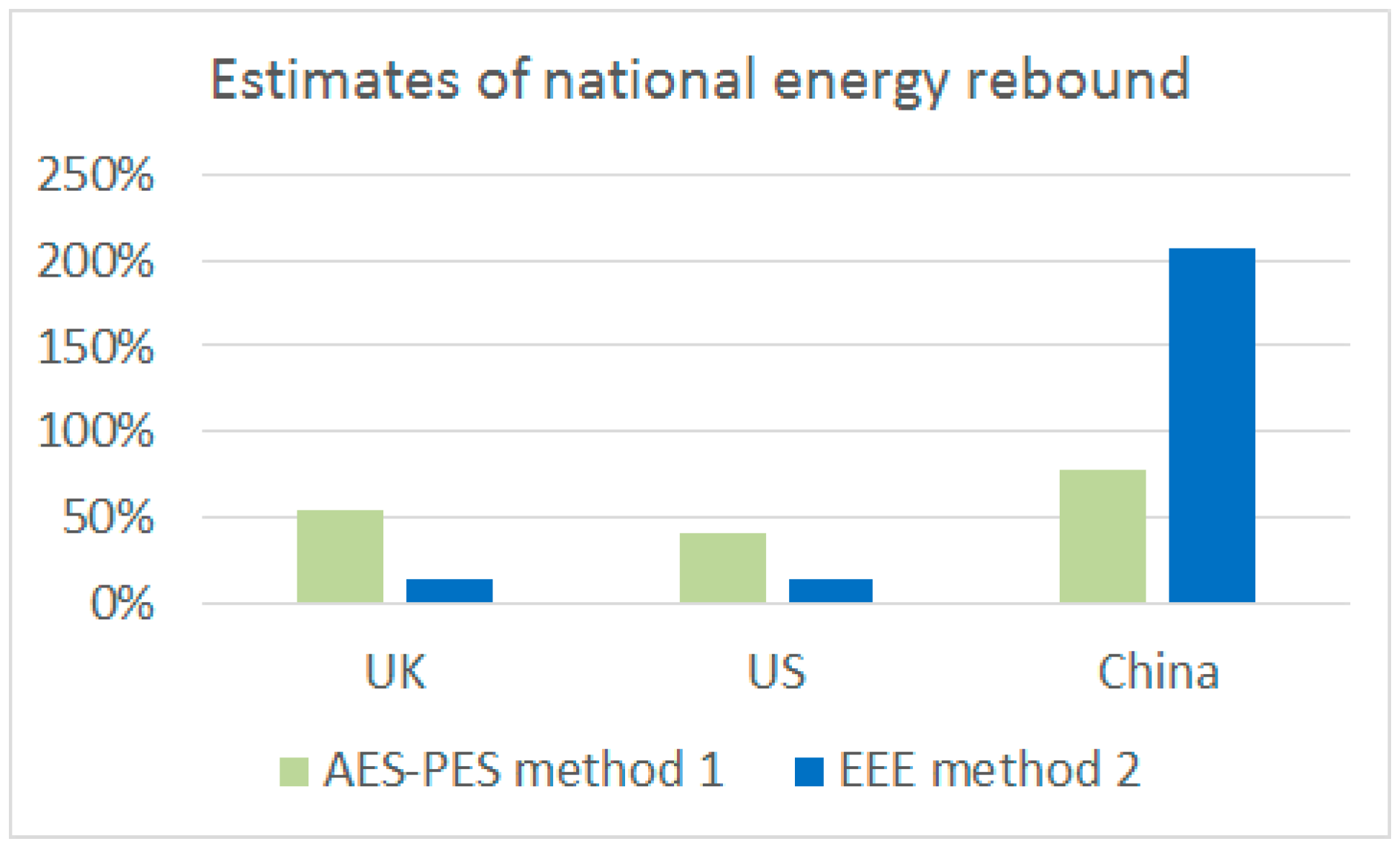
Source (Reference)	Time-Series	Method	Estimate of National Rebound
Shao et al. [73]	1954–2010	AES/PES	37%
Zhang and Lin [33]	1979–2004	AES/PES	41%
	1981–2009	EEE	52% (short term)
Lin and Liu [93]	1981–2009	AES/PES	53%
Li and Lin [94]	1985–2008	AES/PES	67%
Li and Han [95]	1997–2009	AES/PES	74%
Brockway et al. (this study)	1981–2010	AES/PES	77%
Brockway et al. (this study)	1981–2010	EEE	208%

summarises six national rebound estimates found in the literature using AES/PES or EEE methods, plus our own base-fit results. The six AES/PES studies in Table 7 have broadly consistent results: estimating national energy rebound for China to be in the range 37% to 77%, with our value the highest (77%). If we assume that all AES/PES studies (including ours) contain similar aggregate energy intensity (E/GDP) values, it suggests our estimate of λ (exogenous growth term) is higher than the other studies. Certainly, differences would be expected, given all studies obtain values for λ using differing APFs and techniques. Only one other study uses the EEE method—Zhang and Lin [33], however, their estimated value (52%) is for short-term rebound. Whilst Saunders [10] (p. 2208) suggests long term rebound is slightly higher, our EEE-based estimate (208%) is significantly higher, due to a very high elasticity of substitution between KL and E (σ~2.0).

4.2. Interpretation

The key divergence in our results between countries lies in the finding of partial rebound (13%–50%) for UK-US, versus much higher rebound (close to, or above 100%) for China. One explanation may be that 1980–2010 covers the period when China rapidly industrialised—so energy efficiency measures were largely on the producer side, leading to larger rebound—versus the deindustrialising process to more service-based economies of the UK and US. This concept is shown graphically in Figure 11.

There is support in the literature for this view: the IPCC suggests consumer-sided rebound (which we may expect to dominate in a service-based/deindustrialised economy) may be of the order of 20%–45% [104], similar to our (UK-US) results. Meanwhile, Stern [8] describes how producer-sided rebound may be higher as producer responses (i.e., increasing production) are not constrained by a fixed nominal income (as in the case for consumers). Van den Bergh [105] concurs, suggesting developing (or in China’s case—industrialising) countries would have higher rebound than a developed economy due to four factors: higher growth rates; highly intensive energy use; higher cost of energy; and lack of saturation in key energy services such as lighting. All are true of China. Ouyang et al. [106] also highlight the lack of energy service saturation as a key reason for China’s higher energy rebound.

Our fitted values of Hicks elasticity of substitution (σ) between the capital-labour composite and energy also offers some support for this interpretation: σ values were very small for the UK (0.02) and US (0.01), but large for China (2.08). Economic theory suggests where σ is low, energy is not easily substituted for capital-labour, meaning that energy savings (at low σ) would stay largely within the energy sector, yielding smaller rebound. Conversely for larger σ, energy savings are easily replaced by increases in the composite capital-labour inputs, which in turn increases energy use, yielding higher rebound.

Figure 12 examines the influence of the energy cost share (national energy spend/GDP) on the estimates of rebound:

It suggests that China’s rebound is essentially independent of the energy cost share, whereas the UK and US are influenced by the cost-share. The elasticity of substitution value is likely the driving variable, so this finding is reliant on the σ values obtained. Figure 12 also suggests when the energy cost share approaches zero, energy rebound (Re) tends to the value of the elasticity of substitution, σ. This makes sense as, if s_E = 0, then Equation (20) reduces to Equation (22):

$$Re=\frac{1}{\left(1+\mathsf{\rho }\right)}=\mathsf{\sigma }$$

(22)

Further interpretation is found by decomposing Method 2 (EEE) rebound into two parts using Equation (23) (the derivation is in Supplementary Information)—first done by Saunders [10] (p. 2197) In the first part, ${\mathsf{\eta }}_{\mathsf{\tau }}^{E_{Output}}$ depicts the relative change in energy use from changes in output, with energy intensity (E/Y) held constant, whilst ${\mathsf{\eta }}_{\mathsf{\tau }}^{E_{Substitution}}$ captures the substitution (or intensity) effect, i.e., the relative change in energy use from input substitution, with output (Y) held constant.

$${\mathsf{\eta }}_{\mathsf{\tau }}^E={\mathsf{\eta }}_{\mathsf{\tau }}^{E_{Output}}+{\mathsf{\eta }}_{\mathsf{\tau }}^{E_{Substitution}}$$

(23)

Table 8. EEE method rebound—output and substitution components.

Country	Substitution Effect ${\mathsf{\eta }}_{\mathsf{\tau }}^{{\mathit{F}}_{\mathit{S}\mathit{u}\mathit{b}\mathit{s}\mathit{t}\mathit{i}\mathit{t}\mathit{u}\mathit{t}\mathit{i}\mathit{o}\mathit{n}}}$	Re1 = 1 + ${\mathsf{\eta }}_{\mathsf{\tau }}^{{\mathit{F}}_{\mathit{S}\mathit{u}\mathit{b}\mathit{s}\mathit{t}\mathit{i}\mathit{t}\mathit{u}\mathit{t}\mathit{i}\mathit{o}\mathit{n}}}$ (as Decimal Value)	Output Effect ${\mathsf{\eta }}_{\mathsf{\tau }}^{{\mathit{F}}_{\mathit{O}\mathit{u}\mathit{t}\mathit{p}\mathit{u}\mathit{t}}}$	Re = 1 + ${\mathsf{\eta }}_{\mathit{\tau }}^{{\mathit{F}}_{\mathit{S}\mathit{u}\mathit{b}\mathit{s}\mathit{t}\mathit{i}\mathit{t}\mathit{u}\mathit{t}\mathit{i}\mathit{o}\mathit{n}}}+{\mathsf{\eta }}_{\mathit{\tau }}^{{\mathit{F}}_{\mathit{O}\mathit{u}\mathit{t}\mathit{p}\mathit{u}\mathit{t}}}$
				As Decimal Value	As %
UK	−0.98	0.01	0.12	0.13	13%
US	−0.99	0.01	0.12	0.13	13%
China	1.08	2.08	0.00	2.08	208%

presents the rebound results in this split format. Table 8 considers rebound as occurring in two stages. First, is rebound from the substitution effect (i.e., rebound holding output constant). In this case we find negligible rebound for the UK and US (Re₁~1%), versus very high rebound (backfire) for China (Re₁ = 208%). The result for China follows Saunders [10] (p. 2197), who suggested that whereby rebound is governed by substitution effects at high elasticities of substitution. The second (i.e., output effect) component is negligible for China—which needs further exploration, but causes nearly all rebound for the UK and US.

The results also raises the prospect that developed countries who have “offshored” energy-intensive manufacturing industries and thus carbon emissions [107,108] may implicitly also be “offshoring” energy rebound. In our case study, China’s higher rebound (assumed from its producer-sided economy) is therefore due in significant part to the export demands for products manufactured in China from countries including the UK and US. So, in a rebound study based on a consumption-based national rebound approach, we might expect the UK and US rebound to increase, and China’s to reduce.

4.3. Reflections of the Exergy-Based Approaches

This paper has sought to develop and test novel exergy-based approaches to estimate national energy rebound. This is an important aspiration, since national-level rebound studies are rare, and so contributions (as set out in Section 5) are welcome. Reflecting on the exergy-based approaches themselves, whilst sharing a common CES-based framework, it is important to note the two methods are actually very different. This is because they use different independent variables for the estimate of rebound effects—namely endogenous exergy efficiency (τ) and exogenous growth (λ). The former is a direct measure of exergy efficiency improvements, the latter is an estimate of factor-neutral technical change.

There are particular concerns about the ability of the Solow residual ($e^{\mathsf{\lambda }t}$) to capture the rebound effect from energy efficiency alone, since as Shao et al. [73] (p. 239) assert, the Solow residual is “unable to accurately reflect practical technological contribution to economic growth as it contains factors which are too broad”. This is correct: the Solow residual cannot distinguish between the various possible sources of technological change, which may be driven by better managerial skills, augmenting of efficiency units of labour, better matching between capital and labour, or the advance of the technology itself. Thus, energy efficiency may only be part of the rebound picture. On the other hand, “factor-neutral” energy rebound—i.e., capturing the energy rebound from the broad technological change that has actually occurred, whatever its provenance—may actually be desirable, and complementary to “energy efficiency” only rebound. For example, it potentially allows the comparison of “factor-neutral” and “energy efficiency” rebound—similar to Saunders [32]—and by subtraction may be able to isolate the non “energy efficiency” rebound components. Such seemingly divergent approaches may therefore be seen as in a more complementary light.

In addition, our exergy-based approaches have several caveats in common. The first relates to the use of useful exergy as a new approach to the estimation of national energy rebound. There are conceptual reasons for its inclusion (e.g., useful exergy is closer to production processes that are the foundation of economic activity). But there may also reasons for its exclusion—for example if you consider useful exergy is an output of capital equipment (it is thereby not really a primary input) or that it is too closely linked with the adoption of technical change in the production function. In short, further studies and more effort are required to explore its use and potential merit within an energy rebound context.

Second, the exergy efficiency and useful exergy datasets used as inputs to the rebound analysis are based on an approach which lacks a universal, consistent methodology. This is discussed by Sousa et al. [109] and Miller et al. [110], who both highlight several areas for improvement, which—once addressed—will strengthen the approach and provide more robust exergy efficiency datasets. Therefore, the estimation of the CES function parameters (and hence energy rebound) will be affected by any methodological flaws in the exergy-based datasets.

Third, both AES/PES and EEE methods are founded on the econometric estimation of CES-based APFs. Despite their prevalent use in energy-economic modelling to inform policy, the use of APFs can also be viewed as a risk, given there remains a longstanding debate about whether they are meaningful at all [111,112]. Also, though we chose the most rebound flexible APF structure, any limitations of the functional form may propagate to the rebound estimates. For example, amending the approach to account for general equilibrium effects along the lines of Wei [11] may alter the CES parameter values and rebound estimates.

5. Conclusions

Several important steps have been made in this paper. This is the first time that calculated values of aggregate exergy efficiency and useful exergy have been employed in a study of national rebound effects, and the resulting estimates are plausible. An exergy-based approach may help to address Madlener and Alcott’s [113] (p. 374) demand that “some physical metric or metrics enabling a rigorous definition and measurement of macro-level energy efficiency change (e.g., at the national or global level) must be found”. Also, the provision of a multi-method, multi-country empirical study of national energy rebound is in itself noteworthy, as it increases analytical depth and comparability, which serves to broaden the rebound research field. Indeed, to our knowledge only one other KL(U) empirical CES-based study exists [92], so in itself this contributes to other areas such as growth accounting. In addition, the EEE-based energy rebound equation advances Saunders’ [10] existing CES-based rebound equation, as the CES function we adopt is more flexible. The use of resampling also provides an important sense for the precision with which we can determine the CES parameters and estimate of national energy rebound. This is particularly useful given the highly asymmetric resampling intervals obtained for the fitted parameters values, meaning the standard convention of multiplying standard errors by a factor to obtain a symmetric uncertainty interval is not applicable in our case.

From the analysis, we find large energy rebound in China, suggesting that improvements in China’s energy efficiency may be associated with increased energy consumption (“backfire”). Conversely, we find much lower (partial) energy rebound for the case of the UK and US. These findings support the hypothesis that producer-sided economies (such as China) may exist in states of high rebound. This is problematic for climate policy, since if energy efficiency policies are not as effective as planned, this would significantly hamper efforts for energy demand reductions via energy efficiency. Shao et al. [73] suggested that China—in the face of large rebound effects—should further liberalise energy markets coupled to increases in energy taxes. Jenkins et al. [13] (p. 53) concur, advocating taxes should be “sufficient to keep the final price of energy services constant despite improvements in energy efficiency, eliminating any net productivity gains from the efficiency measures”. Returning to the carbon reduction “wedges” of Figure 1, we see how, this would place greater importance on deploying renewable energy sources more rapidly than currently planned, in order to meet climate targets.

Our results also highlight how in higher rebound countries (i.e., China), energy rebound (as the response to energy efficiency measures) may also act as a key component of economic growth. This would follow the advocation of Ayres and Warr [114], who saw energy efficiency (and rebound) as the engine of economic growth. This leads to a potential trade-off, where future economic growth may be restricted by climate-based policies (e.g., carbon taxes) seeking to reduce energy rebound effects.

References

- Intergovernmental Panel on Climate Change (IPCC). Contribution of Working Group III to the Fifth Assessment Report of the Intergovernmental Panel on Climate Change. In Climate Change 2014. Summary for Policymakers; Intergovernmental Panel on Climate Change (IPCC): Cambridge, UK, 2014. [Google Scholar]
- European Parliament. Directive 2009/28/EC of the European Parliament and of the Council of 23 April 2009. Off. J. Eur. Union 2009, 140, 16–62. [Google Scholar]
- European Parliament. Directive 2012/27/EU of the European Parliament and of the Council of 25 October 2012 on energy efficiency. Off. J. Eur. Union 2012, 315, 1–56. [Google Scholar]
- Csereklyei, Z.; Stern, D.I. Global Energy Use: Decoupling or Convergence? Energy Econ. 2015, 51, 633–641. [Google Scholar] [CrossRef]
- Alcott, B. Impact caps: Why population, affluence and technology strategies should be abandoned. J. Clean. Prod. 2010, 18, 552–560. [Google Scholar] [CrossRef]
- Sorrell, S. Energy, economic growth and environmental sustainability: Five propositions. Sustainability 2010, 2, 1784–1809. [Google Scholar] [CrossRef]
- Redrawing the Energy-Climate Map; World Energy Outlook Special Report; International Energy Agency (IEA): Paris, France, 2013.
- Stern, D.I. The role of energy in economic growth. Ann. N. Y. Acad. Sci. 2011, 1219, 26–51. [Google Scholar] [CrossRef] [PubMed]
- Jevons, W.S. The Coal Question: An Inquiry Concerning the Progress of the Nation, and the Probable Exhaustion of Our Coal-Mines, 3rd ed.; Flux, A.W., Ed.; Augustus M. Kelley: New York, NY, USA, 1865. [Google Scholar]
- Saunders, H.D. Fuel conserving (and using) production functions. Energy Econ. 2008, 30, 2184–2235. [Google Scholar] [CrossRef]
- Wei, T. A general equilibrium view of global rebound effects. Energy Econ. 2010, 32, 661–672. [Google Scholar] [CrossRef]
- Greening, L.A.; Greene, D.L.; Difiglio, C. Energy efficiency and consumption—The rebound effect—A survey. Energy Policy 2000, 28, 389–401. [Google Scholar] [CrossRef]
- Jenkins, J.; Nordhaus, T.; Shellenberger, M. Energy Emergence: Rebound and Backfire as Emergent Phenomena; Breakthrough Institute: Oakland, CA, USA, 2011. [Google Scholar]
- Intergovernmental Panel on Climate Change (IPCC). Contribution of Working Group III to the Fifth Assessment Report of the Intergovernmental Panel on Climate Change. In Climate Change 2014: Mitigation of Climate Change; Cambridge University Press: Cambridge, UK, 2014. [Google Scholar]
- Maxwell, D.; Owen, P.; McAndrew, L.; Mudgal, S.; Cachia, F.; Muehmel, K.; Neubauer, A. Addressing the Rebound Effect; Report for the European Commission; Directorate-General (DG) for Environment: Brussels, Belgium, 2011. [Google Scholar]
- Font Vivanco, D.; Kemp, R.; van der Voet, E. How to deal with the rebound effect? A policy-oriented approach. Energy Policy 2016, 94, 114–125. [Google Scholar] [CrossRef]
- UK Energy Bill; Her Majesty’s Government: London, UK, 2012.
- Nørgaard, J.S. Avoiding rebound through a steady-state economy. In Energy Efficiency and Sustainable Consumption: The Rebound Effect; Herring, H., Sorrell, S., Eds.; Palgrave Macmillan: Basingstoke, UK, 2008. [Google Scholar]
- Levett, R. Energy efficiency and sustainable consumption: The rebound effect. In Rebound and Rational Public Policy-Making; Herring, H., Sorrell, S., Eds.; Palgrave Macmillan (St. Martin’s Press): New York, NY, USA, 2009. [Google Scholar]
- Schaefer, S.; Wickert, C. The efficiency paradox in organization and management theory. In Proceedings of the 4th European Theory Development Workshop (EDTW), Cardiff, UK, 25–26 June 2015.
- Sorrell, S. The Rebound Effect: An Assessment of the Evidence for Economy-Wide Energy Savings from Improved Energy Efficiency. UKERC Research Report. Available online: http://www.efslearninghub.net.au/Portals/0/Resources/Publications/Files/565/UK ERC Rebound.pdf (accessed on 30 September 2016).
- Sorrell, S.; Dimitropoulos, J. Review of Evidence for the Rebound Effect Technical Report 2: Econometric Studies; UKERC Work Paper UKERC/WP/TPA/2007/010; The UK Energy Research Centre: London, UK, 2007. [Google Scholar]
- Broadstock, D.C.; Hunt, L.; Sorrell, S. Review of Evidence for the Rebound Effect Technical Report 3: Elasticity of Substitution Studies; UKERC Work Paper UKERC/WP/TPA/2007/011; The UK Energy Research Centre: London, UK, 2007. [Google Scholar]
- Allan, G.; Gilmartin, M.; Turner, K.; McGregor, P.; Swales, K. Review of Evidence for the Rebound Effect Technical Report 4: Computable General Equilibrium Modelling Studies; UKERC Work Paper UKERC/WP/TPA/2007/012; The UK Energy Research Centre: London, UK, 2007. [Google Scholar]
- Sorrell, S.; Dimitropoulos, J. Review of Evidence for the Rebound Effect Technical Report 5: Energy, Productivity and Economic Growth Studies; UKERC Work Paper UKERC/WP/TPA/2007/013; The UK Energy Research Centre: London, UK, 2007. [Google Scholar]
- Stapleton, L.; Sorrell, S.; Schwanen, T. Estimating direct rebound effects for personal automotive travel in Great Britain. Energy Econ. 2016, 54, 313–325. [Google Scholar] [CrossRef]
- Greene, D.L. Rebound 2007: Analysis of U.S. light-duty vehicle travel statistics. Energy Policy 2012, 41, 14–28. [Google Scholar] [CrossRef]
- Druckman, A.; Chitnis, M.; Sorrell, S.; Jackson, T. An Investigation into the Rebound and Backfire Effects from Abatement Actions by UK Households. Available online: http://epubs.surrey.ac.uk/729052/1/RESOLVE WP 05-10.pdf (accessed on 30 September 2016).
- Azevedo, I.L.; Sonnberger, M.; Thomas, B.; Morgan, G.; Renn, O. The Rebound Effect: Implications of Consumer Behaviour for Robust Energy Policies; International Risk Governance Council: Lausanne, Switzerland, 2013. [Google Scholar]
- Bentzen, J. Estimating the rebound effect in US manufacturing energy consumption. Energy Econ. 2004, 26, 123–134. [Google Scholar] [CrossRef]
- Saunders, H.D. Historical evidence for energy efficiency rebound in 30 US sectors and a toolkit for rebound analysts. Technol. Forecast. Soc. Chang. 2013, 80, 1317–1330. [Google Scholar] [CrossRef]
- Saunders, H.D. Recent Evidence for Large Rebound: Elucidating the Drivers and their Implications for Climate Change Models. Energy J. 2015, 36, 23–48. [Google Scholar] [CrossRef]
- Zhang, J.; Lin, C.C. Estimating the Macroeconomic Rebound Effect in China. UC Davis Work Paper. 2013. Available online: http//www.des.ucdavis.edu/faculty/lin/china_rebound_effect_paper.pdf (accessed on 30 September 2016).
- Fouquet, R. Long-Run Demand for Energy Services: Income and Price Elasticities over Two Hundred Years. Rev. Environ. Econ. Policy 2014, 8, 186–207. [Google Scholar] [CrossRef]
- Fouquet, R.; Pearson, P.J.G. The Long Run Demand for Lighting: Elasticities and Rebound Effects in Different Phases of Economic Development. Econ. Energy Environ. Policy 2011, 1, 83–100. [Google Scholar]
- Tsao, J.Y.; Saunders, H.D.; Creighton, J.R.; Coltrin, M.E.; Simmons, J.A. Solid-state lighting: An energy-economics perspective. J. Phys. D Appl. Phys. 2010, 43, 354001. [Google Scholar] [CrossRef]
- HM Revenue and Customs. HMRC’s CGE Model Documentation. 2013. Available online: https://www.gov.uk/government/uploads/system/uploads/attachment_data/file/263652/CGE_model_doc_131204_new.pdf (accessed on 30 September 2016). [Google Scholar]
- Barker, T.; Dagoumas, A.; Rubin, J. The macroeconomic rebound effect and the world economy. Energy Effic. 2009, 2, 411–427. [Google Scholar] [CrossRef]
- International Energy Agency (IEA). World Energy Model Documentation 2013 Version. Available online: http://www.worldenergyoutlook.org/media/weowebsite/2013/WEM_Documentation_WEO2013.pdf (accessed on 30 September 2016).
- Rant, Z. Exergy, a new word for “technical available work”. Forsch. Ing. 1956, 22, 36–37. [Google Scholar]
- Reistad, G. Available Energy Conversion and Utilization in the United States. ASME Trans. Ser. J. Eng. Power 1975, 97, 429–434. [Google Scholar] [CrossRef]
- Ford, K.W.; Rochlin, G.I.; Socolow, R.H.; Hartley, D.L.; Hardesty, D.R.; Lapp, M.; Dooher, J.; Dryer, F.; Berman, S.M.; Silverstein, S.D. Technical Aspects of the More Efficient Utilization of Energy: Chapter 2—Second law efficiency: The role of the second law of thermodynamics in assessing the efficiency of energy use. Am. Inst. Phys. Conf. 1975, 25, 25–51. [Google Scholar]
- Ford, K.W.; Rochlin, G.I.; Socolow, R.H.; Hartley, D.L.; Hardesty, D.R.; Lapp, M.; Dooher, J.; Dryer, F.; Berman, S.M.; Silverstein, S.D. Technical Aspects of the More Efficient Utilization of Energy: Chapter 4—The automobile. Am. Inst. Phys. Conf. 1975, 25, 99–120. [Google Scholar]
- Ford, K.W.; Rochlin, G.I.; Socolow, R.H.; Hartley, D.L.; Hardesty, D.R.; Lapp, M.; Dooher, J.; Dryer, F.; Berman, S.M.; Silverstein, S.D. Technical Aspects of the More Efficient Utilization of Energy: Chapter 5—Sample industrial processes. Am. Inst. Phys. Conf. 1975, 25, 122–159. [Google Scholar]
- Georgescu-Roegen, N. The Entropy Law and the Economic Process; Harvard University: Cambridge, MA, USA, 1971. [Google Scholar]
- Georgescu-Roegen, N. Energy and Economic Myths. South Econ. J. 1975, 41, 347–381. [Google Scholar] [CrossRef]
- Georgescu-Roegen, N. Energy Analysis and Economic Valuation. South Econ. J. 1979, 45, 1023–1058. [Google Scholar] [CrossRef]
- Ayres, R. The minimum complexity of endogenous growth models: The role of physical resource flows. Energy 2001, 26, 817–838. [Google Scholar] [CrossRef]
- Ayres, R.U.; Ayres, L.W.; Warr, B. Exergy, power and work in the US economy, 1900–1998. Energy 2003, 28, 219–273. [Google Scholar] [CrossRef]
- Ayres, R.U.; Warr, B. Accounting for growth: The role of physical work. Struct. Chang. Econ. Dyn. 2005, 16, 181–209. [Google Scholar] [CrossRef]
- Warr, B.; Ayres, R.U. Useful work and information as drivers of economic growth. Ecol. Econ. 2012, 73, 93–102. [Google Scholar] [CrossRef]
- Serrenho, A.C.; Warr, B.; Sousa, T.; Ayres, R.U. Structure and dynamics of useful work along the agriculture-industry-services transition: Portugal from 1856 to 2009. Struct. Chang. Econ. Dyn. 2016, 36, 1–21. [Google Scholar] [CrossRef]
- Brockway, P.E.; Barrett, J.R.; Foxon, T.J.; Steinberger, J.K. Divergence of trends in US and UK aggregate exergy efficiencies 1960–2010. Environ. Sci. Technol. 2014, 48, 9874–9881. [Google Scholar] [CrossRef] [PubMed]
- Ayres, R.; Voudouris, V. The economic growth enigma: Capital, labour and useful energy? Energy Policy 2014, 64, 16–28. [Google Scholar] [CrossRef]
- Serrenho, A.C.; Sousa, T.; Warr, B.; Ayres, R.U.; Domingos, T. Decomposition of useful work intensity: The EU (European Union)-15 countries from 1960 to 2009. Energy 2014, 76, 704–715. [Google Scholar] [CrossRef]
- Brockway, P.E.; Barrett, J.R.; Foxon, T.J.; Steinberger, J.K. Supporting Information—Divergence of trends in US and UK aggregate exergy efficiencies 1960–2010. Environ. Sci. Technol. 2014, 48, S1–S39. [Google Scholar] [CrossRef] [PubMed]
- Patterson, M.G. What is energy efficiency? Energy Policy 1996, 24, 377–390. [Google Scholar] [CrossRef]
- Malpede, M.; Verdolini, E. Rebound Effects in Europe. In Proceedings of the Fourth IAERE Annual Conference, Bologna, Italy, 11–12 February 2016.
- Szargut, J.; Morris, D.R.; Steward, F.R. Exergy Analysis of Thermal, Chemical and Metallurgical Processes; Hemisphere: New York, NY, USA, 1988. [Google Scholar]
- Warr, B.; Ayres, R.; Eisenmenger, N.; Krausmann, F.; Schandl, H. Energy use and economic development: A comparative analysis of useful work supply in Austria, Japan, the United Kingdom and the US during 100 years of economic growth. Ecol. Econ. 2010, 69, 1904–1917. [Google Scholar] [CrossRef]
- Lloyd, P.J. The Origins of the von Thünen-Mill-Wiksell-Cobb-Douglas Function. Hist. Polit. Econ. 2001, 33, 1–19. [Google Scholar] [CrossRef]
- Mishra, S.K. A Brief History of Production Functions. IUP J. Manag. Econ. 2010, VIII, 6–34. [Google Scholar] [CrossRef]
- Miller, E. An Assessment of CES and Cobb-Douglas Production Functions; US Congressional Budget Office Work Paper 2008-05; Congressional Budget Office: Washington, DC, USA, 2008.
- Solow, R.M. Technical Change and the Aggregate Production Function. Rev. Econ. Stat. 1957, 39, 312–320. [Google Scholar] [CrossRef]
- Denison, E.F. Accounting for Slower Economic Growth: The United States in the 1970’s; Brookings Institution Press: Washington, DC, USA, 1979. [Google Scholar]
- Barro, R.J. Notes on growth accounting. J. Econ. Growth 1999, 4, 119–137. [Google Scholar] [CrossRef]
- Manne, A.; Mendelsohn, R.; Richels, R. MERGE. A model for evaluating regional and global effects of GHG reduction policies. Energy Policy 1995, 23, 17–34. [Google Scholar] [CrossRef]
- Arora, V. An Evaluation of Macroeconomic Models for Use at EIA; U.S. Energy Information Administration: Washington, DC, USA, 2013.
- Klump, R.; Mcadam, P.; Willman, A. The Normalised CES Production Function: Theory and Empirics; European Central Bank Work Paper 1294; European Central Bank: Frankfurt, Germany, 2011. [Google Scholar]
- Growiec, J. On the Measurement of Technological Progress across Countries; National Bank of Poland Work Paper No. 73; National Bank of Poland: Warsaw, Poland, 2010. [Google Scholar]
- Groth, B.C.; Gutierrez-domenech, M.; Srinivasan, S. Measuring total factor productivity for the United Kingdom. Bank Engl. Q. Bull. Spring 2004, 2004, 63–73. [Google Scholar]
- Cambridge Centre for Climate Change Mitigation Research (4CMR). The Macro-Economic Rebound Effect and the UK Economy. 2006. Available online: http://ukerc.rl.ac.uk/pdf/ee01015_final_b.pdf (accessed on 30 September 2016).
- Shao, S.; Huang, T.; Yang, L. Using latent variable approach to estimate China’s economy-wide energy rebound effect over 1954–2010. Energy Policy 2014, 72, 235–248. [Google Scholar] [CrossRef]
- Sorrell, S. Energy Substitution, Technical Change and Rebound Effects. Energies 2014, 7, 2850–2873. [Google Scholar] [CrossRef]
- Van der Werf, E. Production functions for climate policy modeling: An empirical analysis. Energy Econ. 2008, 30, 2964–2979. [Google Scholar] [CrossRef]
- Warr, B.S.; Ayres, R.U. Evidence of causality between the quantity and quality of energy consumption and economic growth. Energy 2010, 35, 1688–1693. [Google Scholar] [CrossRef]
- Voudouris, V.; Ayres, R.; Serrenho, A.C.; Kiose, D. The economic growth enigma revisited: The EU-15 since the 1970s. Energy Policy 2015, 86, 812–832. [Google Scholar] [CrossRef]
- Temple, J. The calibration of CES production functions. J. Macroecon. 2012, 34, 294–303. [Google Scholar] [CrossRef]
- Feenstra, R.C.; Inklaar, R.; Timmer, M.P. Penn World Tables 8.1. 2015. Available online: http://www.rug.nl/research/ggdc/data/pwt/pwt-8.1 (accessed on 30 September 2016).
- Nilsen, Ø.A.; Raknerud, A.; Rybalka, M.; Skjerpen, T. The importance of skill measurement for growth accounting. Rev. Income Wealth 2011, 57, 293–305. [Google Scholar] [CrossRef]
- Daude, C. Understanding Solow Residuals in Latin America. Economia 2014, 13, 109–138. [Google Scholar]
- Hájková, D.; Hurník, J. Cobb-Douglas production function: The case of a converging economy. Czech J. Econ. Financ. 2007, 57, 465–476. [Google Scholar]
- Barro, R.; Lee, J.-W. Barro-Lee Educational Attainment Dataset Version 2.0. 2014. Available online: http://www.barrolee.com/ (accessed on 30 September 2016).
- Wu, H.X. China’s Growth and Productivity Performance Debate Revisited—Accounting for China’s Sources of Growth with a New Data Set. 2014. Available online: https//www.conference-board.org/pdf_free/workingpapers/EPWP1401.pdf (accessed on 30 September 2016).
- Wallis, G.; Oulton, N. Integrated Estimates of Capital Stocks and Services for the United Kingdom: 1950–2013; CEP Discussion Papers, CEPDP1342; Centre for Economic Performance, London School of Economics and Political Science: London, UK.
- US Bureau of Labour Statistics. Total Economy Production Account and Costs, 1987 to 2013. 2015. Available online: http://www.bls.gov/mfp/special_requests/prod3.totecotable.zip (accessed on 30 September 2016). [Google Scholar]
- Schreyer, P.; Bignon, P.; Dupont, J. OECD Capital Services Estimates: Methodology and a First Set of Results; OECD Statistics Working Papers 2003/06; OECD Publishing: Paris, France, 2003. [Google Scholar]
- Wu, H.X. Constructing China’s Net Capital and Measuring Capital Services in China, 1980–2010; Discussion Papers 15-E-006; Research Institute of Economy, Trade and Industry (RIETI): Tokyo, Japan, 2015; pp. 1–39.
- Brockway, P.E.; Steinberger, J.K.; Barrett, J.R.; Foxon, T.J. Understanding China’s past and future energy demand: An exergy efficiency and decomposition analysis. Appl. Energy 2015, 155, 892–903. [Google Scholar] [CrossRef]
- Henningsen, A.; Henningsen, G. Econometric Estimation of the “Constant Elasticity of Substitution” Function in R: Package micEconCES; FOI Working Paper 2011/9; Institute of Food and Resource Economics, University of Copenhagen: Frederiksberg, Denmark, 2011. [Google Scholar]
- Henningsen, A.; Henningsen, G. On estimation of the CES production function—Revisited. Econ. Lett. 2012, 115, 67–69. [Google Scholar] [CrossRef] [Green Version]
- Heun, M.K.; Santos, J.; Brockway, P.E.; Pruim, R.; Domingos, T. From theory to econometrics to energy policy: Cautionary tales for policymaking using aggregate production functions. Energies 2016. submitted for publication. [Google Scholar]
- Lin, B.; Liu, X. Dilemma between economic development and energy conservation: Energy rebound effect in China. Energy 2012, 45, 867–873. [Google Scholar] [CrossRef]
- Li, L.; Lin, X. Regional Energy Rebound Effect in China Based on IPAT Equation. In Proceedings of the 2012 Asia-Pacific Power and Energy Engineering Conference, Shanghai, China, 27–29 March 2012; pp. 1–4.
- Li, L.; Yonglei, H. The Energy Efficiency Rebound Effect in China from Three Industries Perspective. Energy Procedia 2012, 14, 1105–1110. [Google Scholar] [CrossRef]
- International Energy Agency (IEA). “Extended World Energy Balances”, IEA World Energy Statistics and Balances (Database). 2013. Available online: http://www.oecd-ilibrary.org/energy/data/iea-world-energy-statistics-and-balances/extended-world-energy-balances_data-00513-en (accessed on 30 September 2016).
- Hogan, W.W.; Manne, A.S. Energy-Economy Interactions: The Fable of the Elephant and the Rabbit? Stanford University: Stanford, CA, USA, 1977. [Google Scholar]
- Platchkov, L.M.; Pollitt, M.G. The Economics of Energy (and Electricity) Demand; Working Paper 1116; University of Cambridge Electricity Policy Research Group: Cambridge, UK, 2011. [Google Scholar]
- US Energy Information Administration (US EIA). Energy Consumption, Expenditures, and Emissions Indicators Estimates, Selected Years, 1949–2011. U.S. Energy Information Administration/Annual Energy Review 2011. Available online: http://www.eia.gov/totalenergy/data/annual/pdf/sec1_13.pdf (accessed on 30 September 2016).
- Schneider, D. The Labor Share: A Review of Theory and Evidence. 2011. Available online: http://edoc.hu-berlin.de/series/sfb-649-papers/2011-69/PDF/69.pdf (accessed on 30 September 2016).
- Qi, H. The Labor share question in China. Available online: http://monthlyreview.org/2014/01/01/labor-share-question-china/ (accessed on 30 September 2016).
- Barker, T.; Ekins, P.; Foxon, T. The macro-economic rebound effect and the UK economy. Energy Policy 2007, 35, 4935–4946. [Google Scholar] [CrossRef]
- Sorrell, S. Jevons’ Paradox revisited: The evidence for backfire from improved energy efficiency. Energy Policy 2009, 37, 1456–1469. [Google Scholar] [CrossRef]
- Climate Change 2014: Mitigation of Climate Change; Working Group III Contribute to Fifth Assessment Report. Intergovernmental Panel Climate Change (IPCC). Available online: http://www.ipcc.ch/report/ar5/wg3/ (accessed on 30 September 2016).
- Van den Bergh, J.C.J.M. Energy Conservation More Effective With Rebound Policy. Environ. Resour. Econ. 2011, 48, 43–58. [Google Scholar] [CrossRef]
- Ouyang, J.; Long, E.; Hokao, K. Rebound effect in Chinese household energy efficiency and solution for mitigating it. Energy 2010, 35, 5269–5276. [Google Scholar] [CrossRef]
- Levinson, A. Offshoring Pollution: Is the United States Increasingly Importing Polluting Goods? Rev. Environ. Econ. Policy 2009, 4, 63–83. [Google Scholar] [CrossRef]
- Peters, G.P.; Minx, J.C.; Weber, C.L.; Edenhofer, O. Growth in emission transfers via international trade from 1990 to 2008. Proc. Natl. Acad. Sci. USA 2011, 108, 8903–8908. [Google Scholar] [CrossRef] [PubMed]
- Sousa, T.; Brockway, P.E.; Cullen, J.M.; Serrenho, A.C.; Henriques, S.T.; Domingos, T. Improving the Robustness of Societal Exergy Accounting. Energy 2016. submitted for publication. [Google Scholar]
- Miller, J.; Foxon, T.; Sorrell, S. Exergy Accounting: A Quantitative Comparison of Methods and Implications for Energy-Economy Analysis. Energies 2016, 9, 947. [Google Scholar] [CrossRef]
- Felipe, J.; Mccombie, J.S.L. How Sound are the Foundations of the Aggregate Production Function? East. Econ. J. 2005, 31, 467–488. [Google Scholar]
- Felipe, J.; McCombie, J.S.L. The Aggregate Production Function: “Not Even Wrong”. Rev. Polit. Econ. 2014, 26, 60–84. [Google Scholar] [CrossRef]
- Madlener, R.; Alcott, B. Energy rebound and economic growth: A review of the main issues and research needs. Energy 2009, 34, 370–376. [Google Scholar] [CrossRef]
- Ayres, R.U.; Warr, B. The Economic Growth Engine: How Energy and Work Drive Material Prosperity; Edward Elgar: Cheltenham, UK, 2010. [Google Scholar]