
Assessment against Experiments of Devolatilization and Char Burnout Models for the Simulation of an Aerodynamically Staged Swirled Low-NOx Pulverized Coal Burner

 ,
,
Abstract
:1. Introduction
2. Experimental Activity
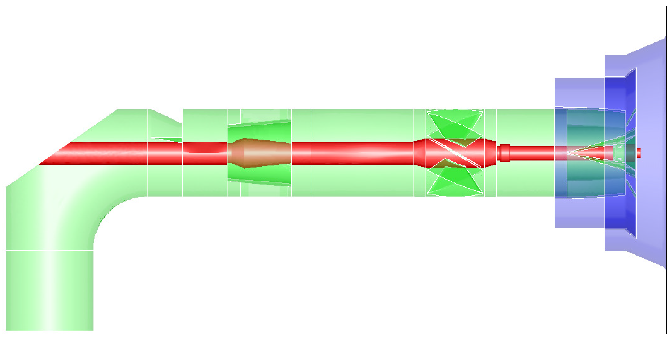
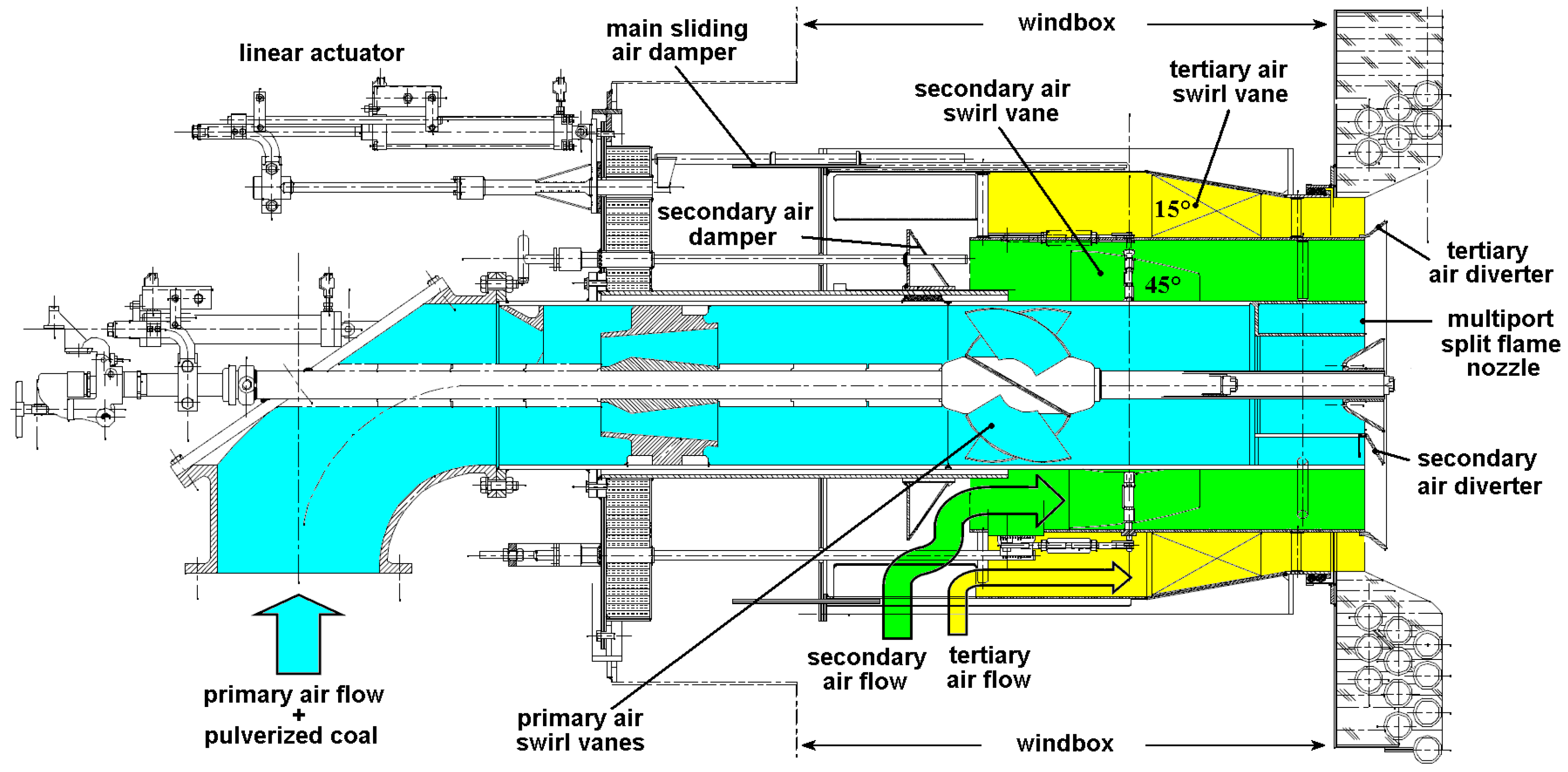
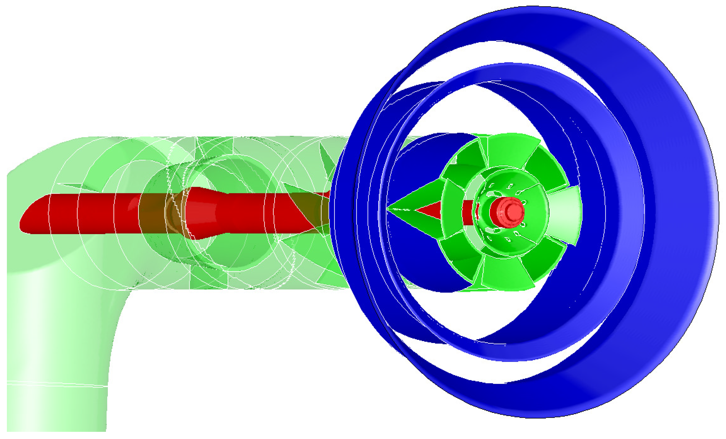
2.1. The Burner
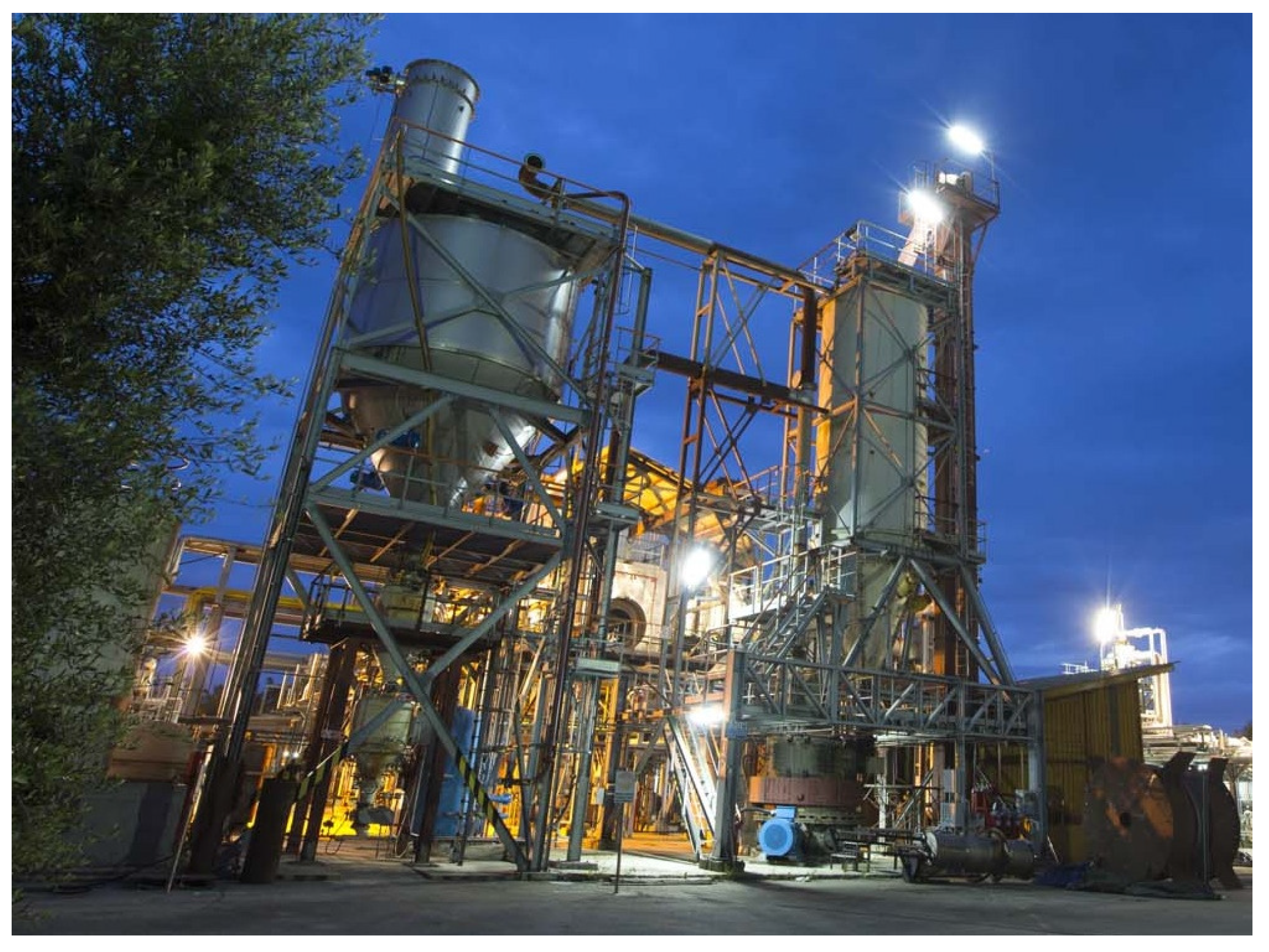
2.2. The CCA Test Facility
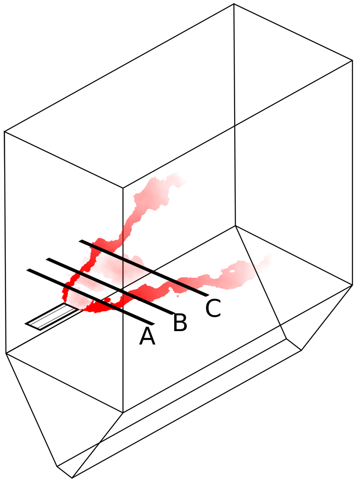
2.3. The Measuring Equipment and Technologies
3. Numerical Model
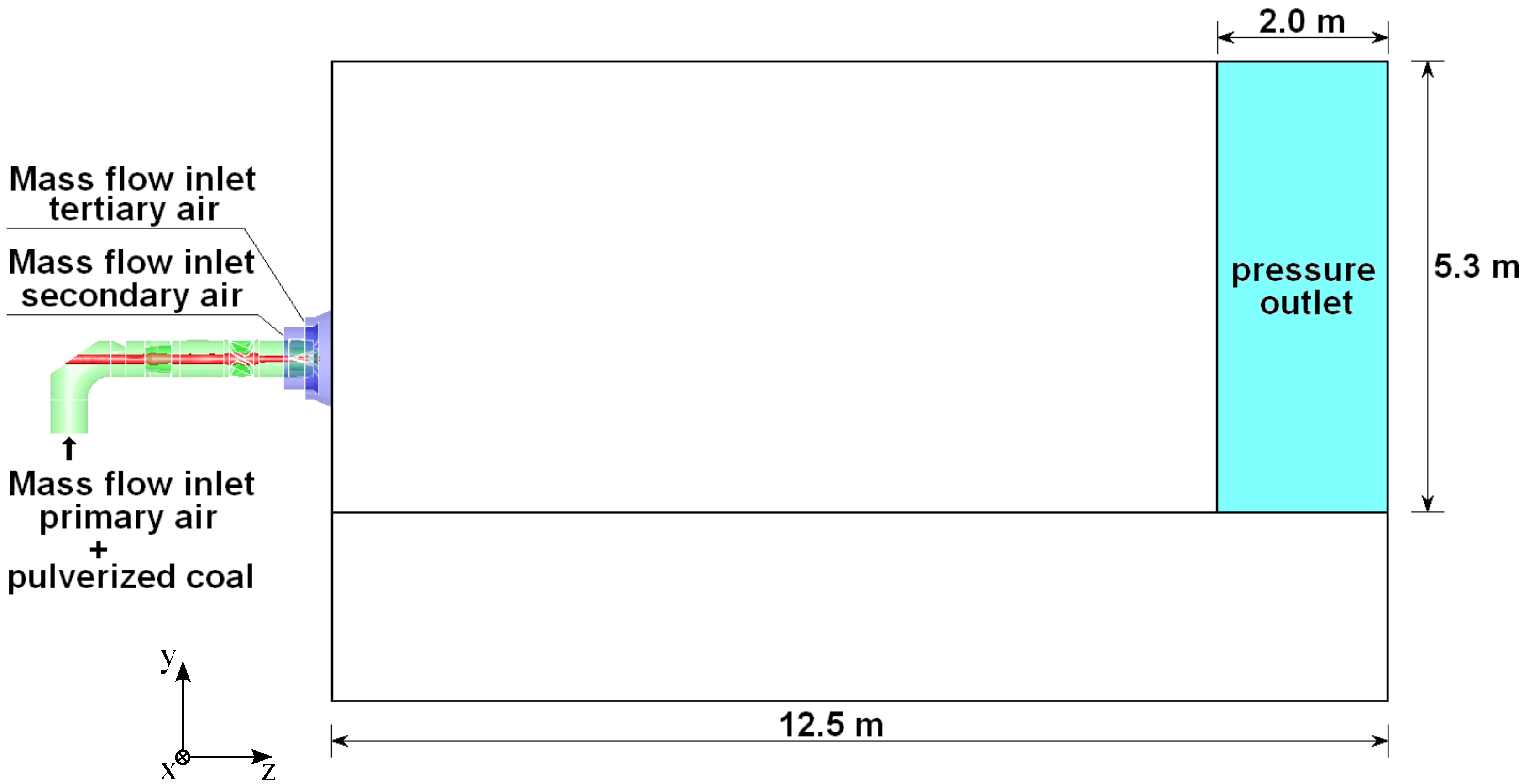
3.1. Boundary Conditions
3.2. Radiation Heat Transfer
3.3. Pulverized Coal Combustion
3.3.1. Devolatilization Models
Single Kinetic Rate Model
Chemical Percolation Devolatilization Model
3.3.2. Char Burnout Models
Kinetic/Diffusion-Limited Surface Reaction Rate Model
Intrinsic Model
3.4. NO Emission Models
3.4.1. Thermal NO Model
3.4.2. Fuel NO Model
4. Results
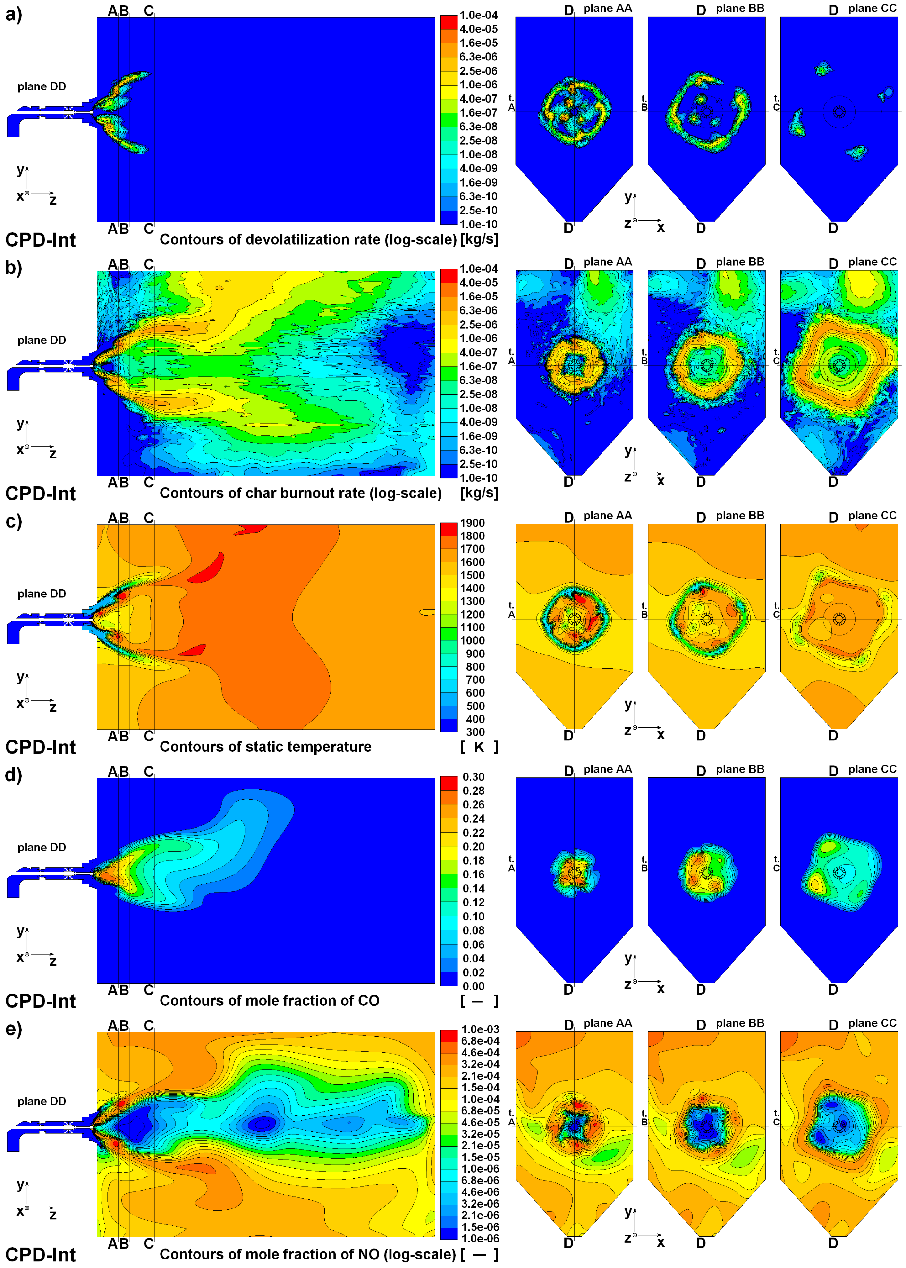
4.1. Simulation 1: CPD-Int Models
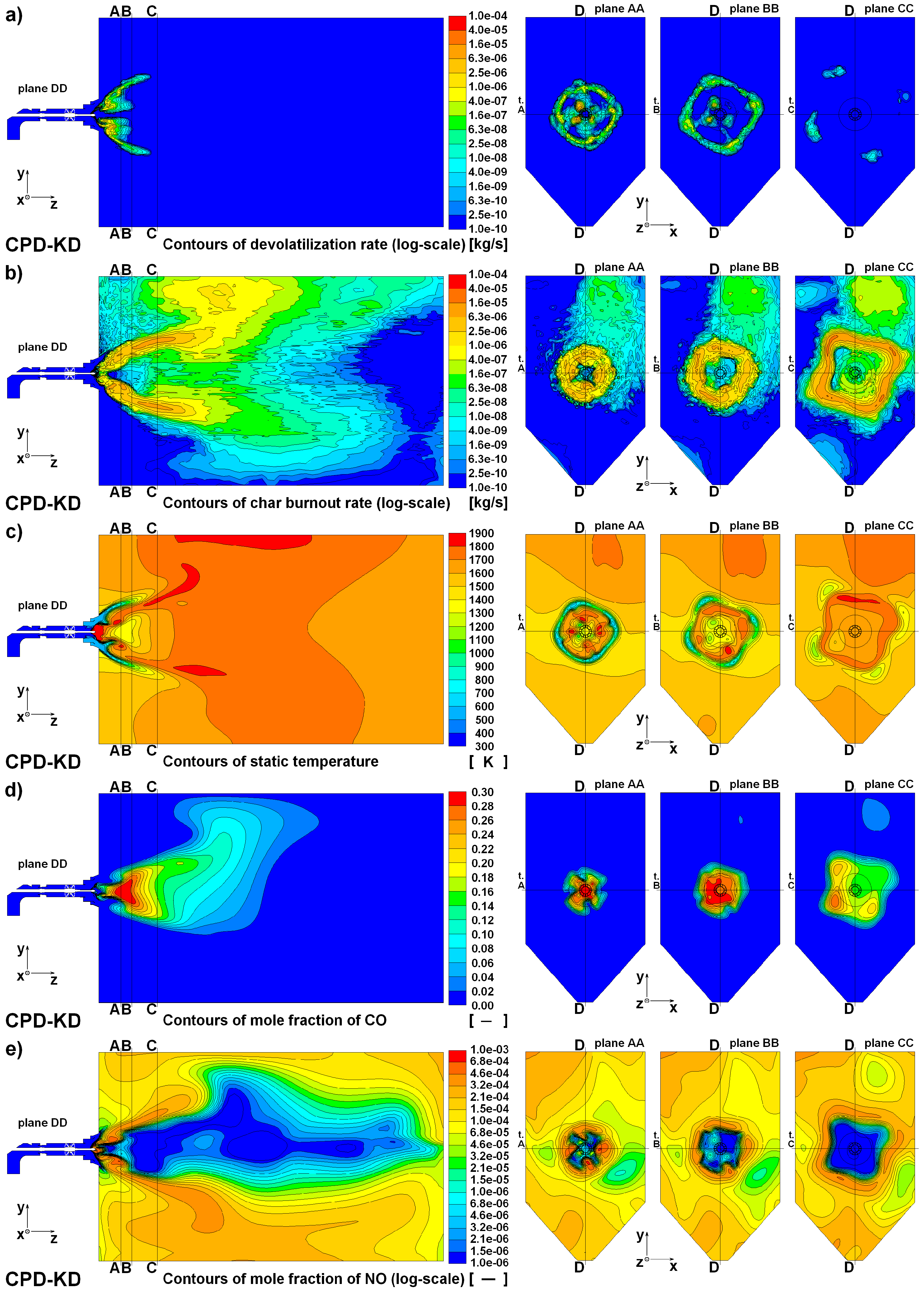
4.2. Simulation 2: CPD-KD Models
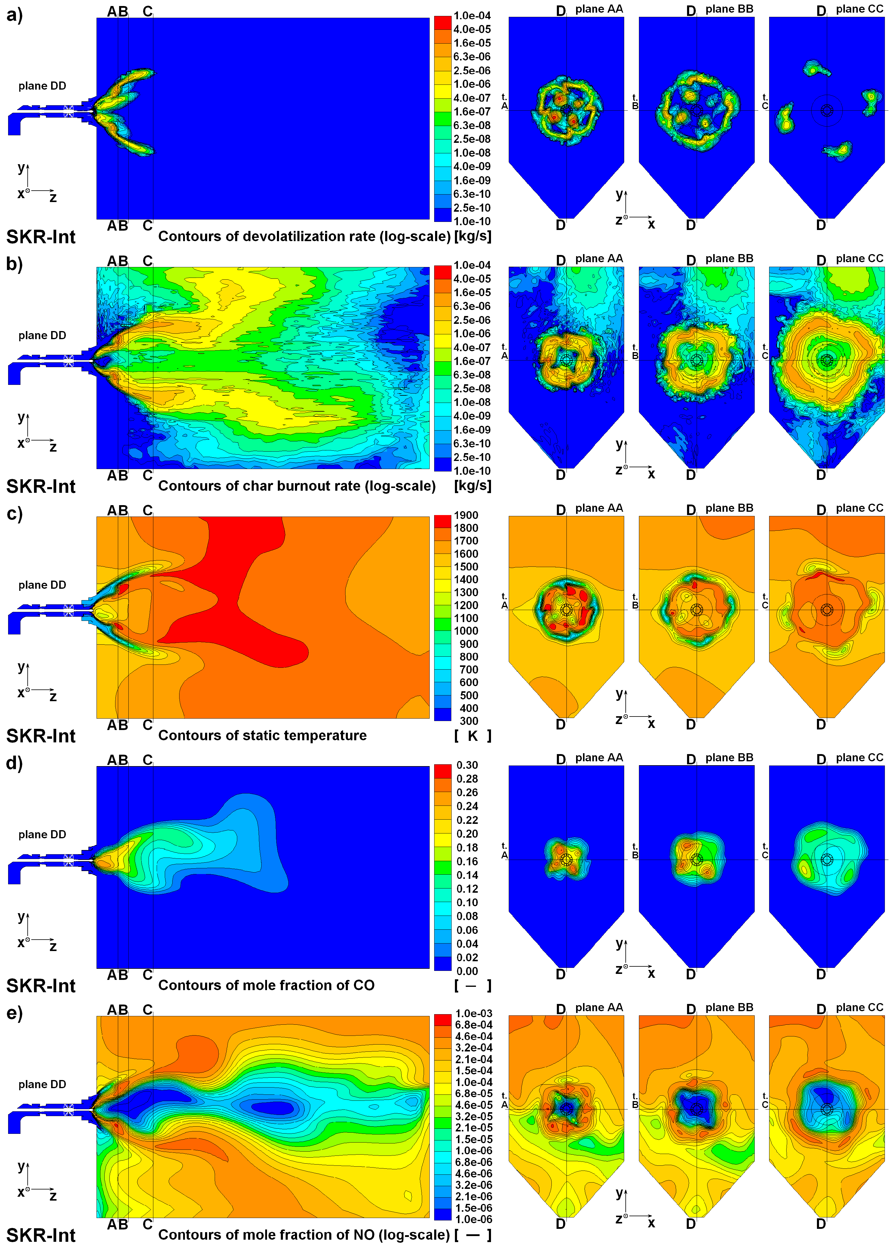
4.3. Simulation 3: SKR-Int Models
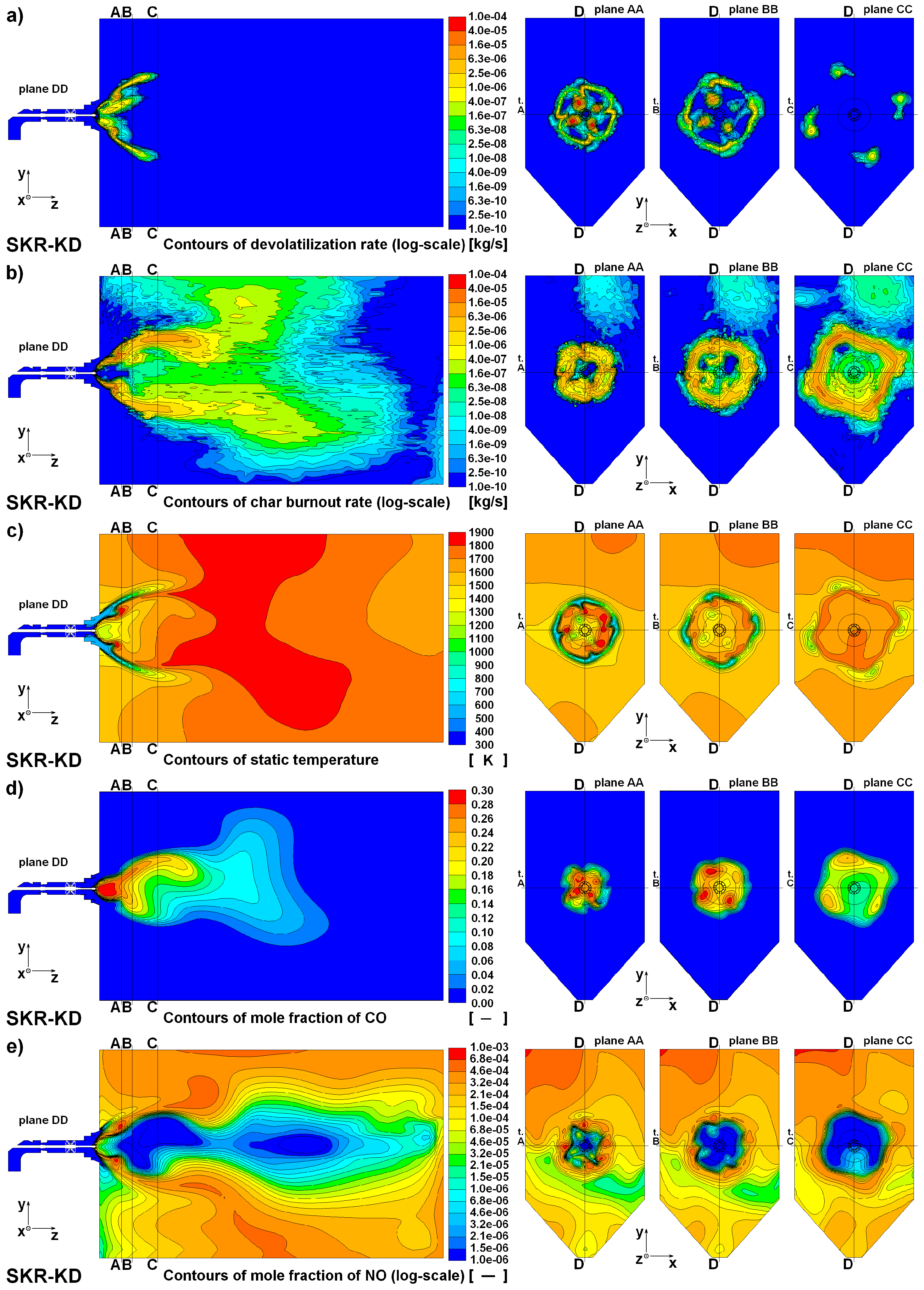
4.4. Simulation 4: SKR-KD Models
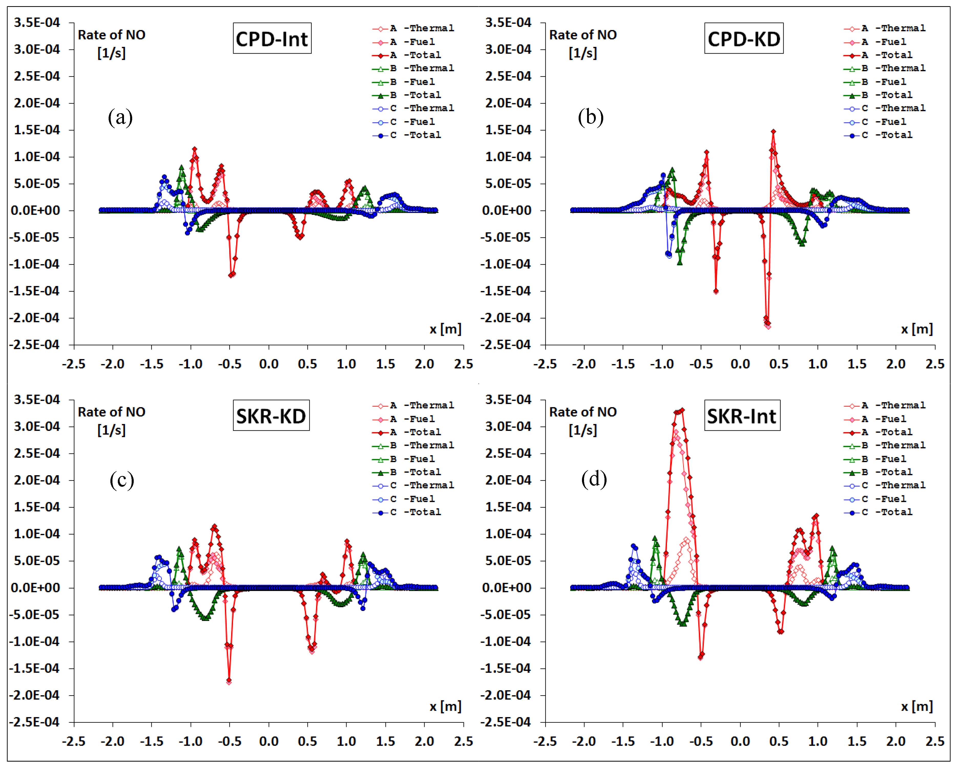
4.5. Rate of Formation of NO
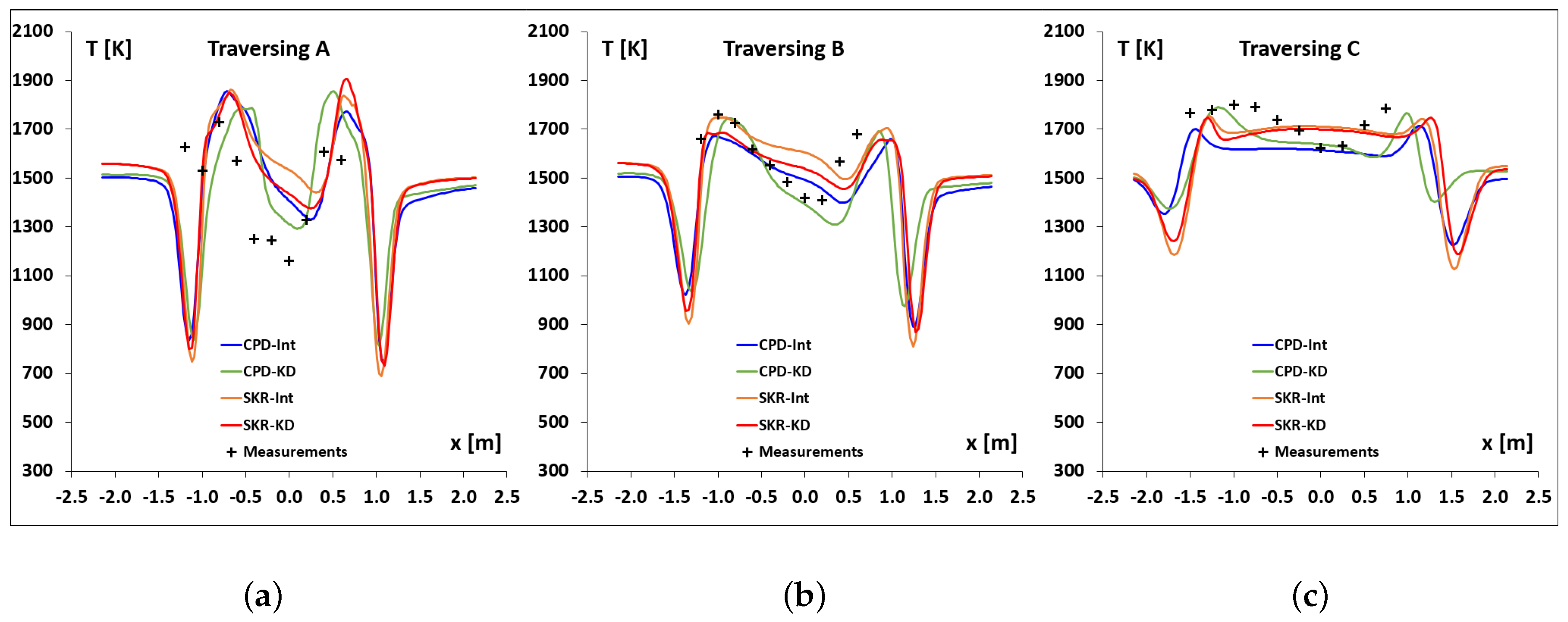
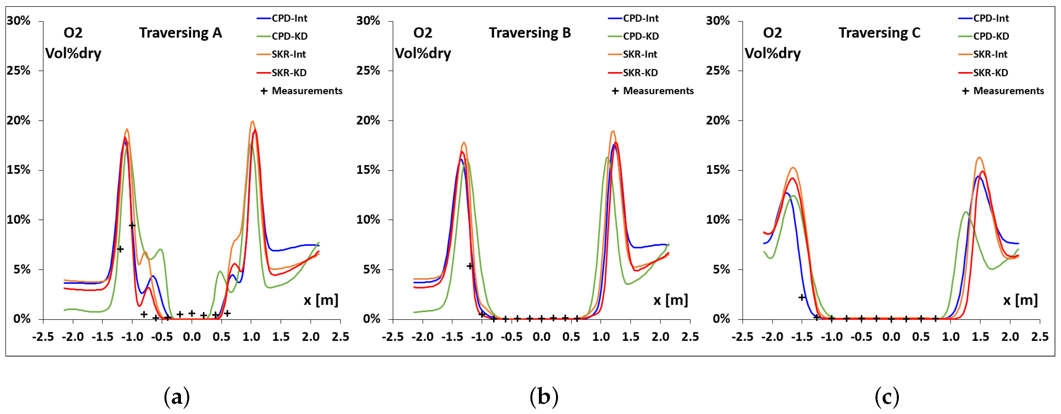
4.6. Assessment of the Models
4.6.1. Temperature and O
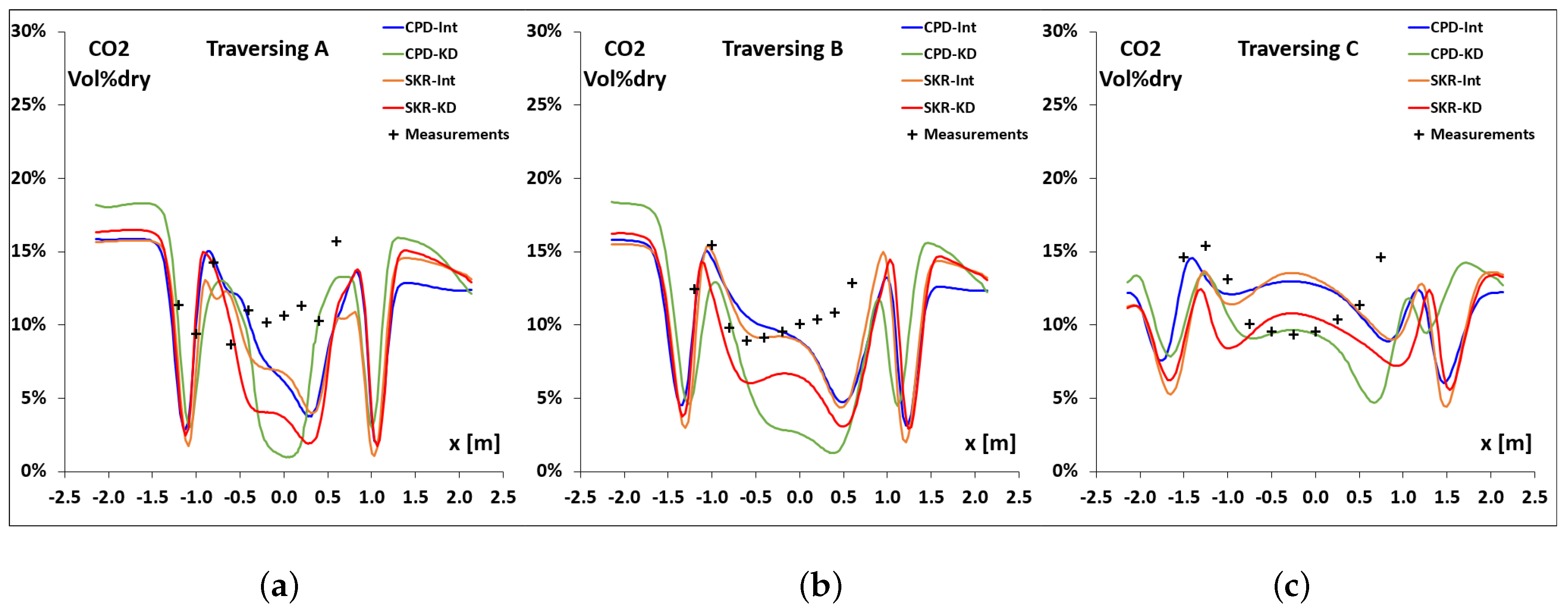
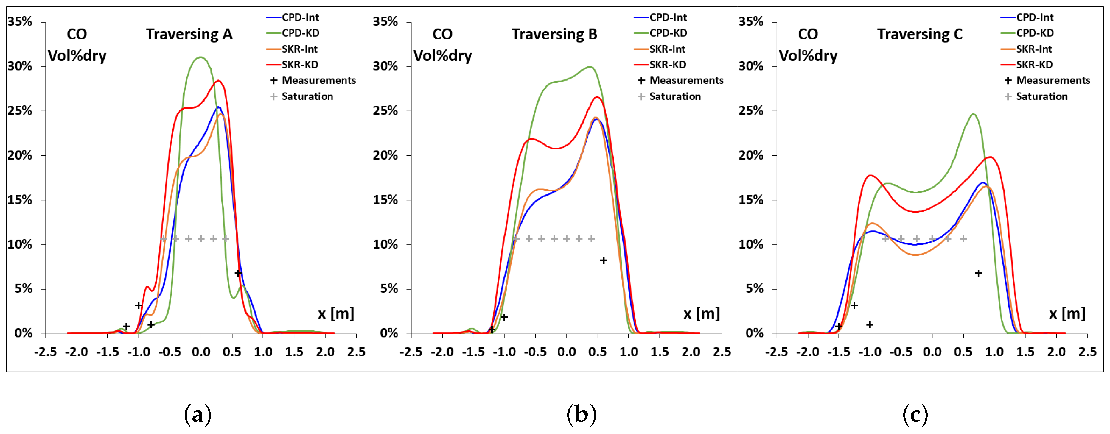
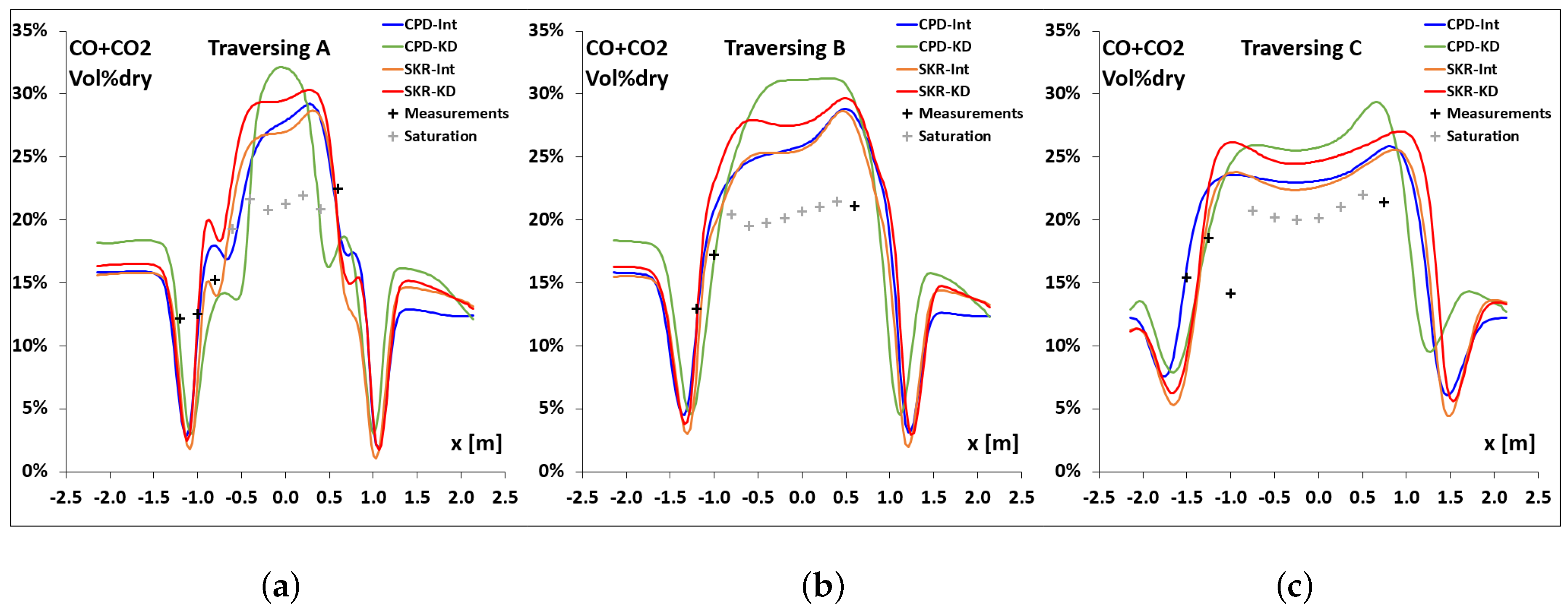
4.6.2. CO and CO
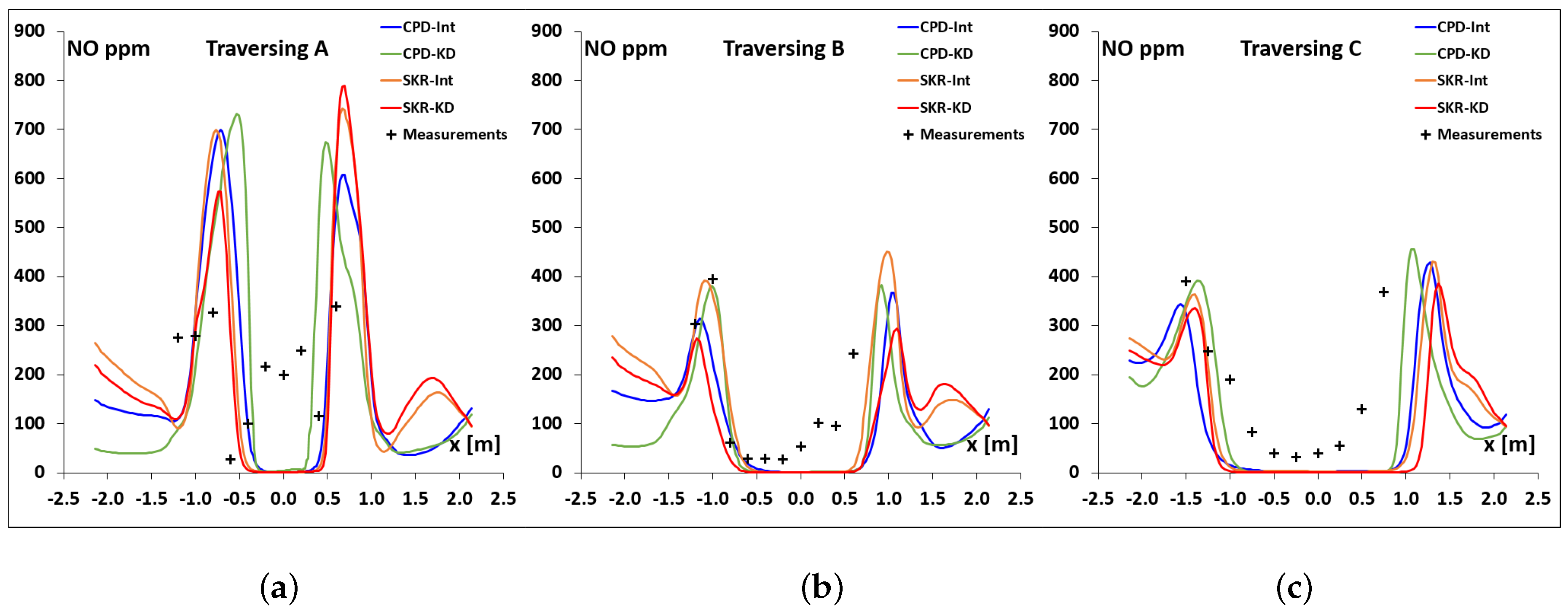
4.6.3. NO
5. Conclusions
Acknowledgments
Author Contributions
Conflicts of Interest
Abbreviations
| Primary mass flow rate | |
| Primary inlet temperature | |
| Primary turbulence intensity | |
| Primary hydraulic diameter | |
| Secondary mass flow rate | |
| Secondary velocity angle | |
| Secondary inlet temperature | |
| Secondary turbulence intensity | |
| Secondary hydraulic diameter | |
| Tertiary mass flow rate | |
| Tertiary velocity angle | |
| Tertiary inlet temperature | |
| Tertiary turbulence intensity | |
| Tertiary hydraulic diameter | |
| Coal mass flow rate | |
| Vaporization temperature | |
| Volatile fraction | |
| Particle mass | |
| Swelling coefficient | |
| Arrhenius activation energy | |
| A | Arrhenius pre-exponential factor |
| Diffusion rate coefficient | |
| R | Kinetic rate coefficient |
| Mass diffusion-limited rate constant | |
| Kinetic-limited rate pre-Exp. factor | |
| Kinetic-limited rate Activ. energy | |
| Char porosity | |
| Mean pore radius | |
| Specific internal surface area | |
| Tortuosity | |
| Burning mode | |
| Coal density | |
| Coal specific heat | |
| mineral matter free | |
| dry mineral matter free | |
| Low heating value |
References
- BP Statistical Review of World Energy, June 2016. Available online: https://www.bp.com/content/dam/bp/pdf/energy-economics/statistical-review-2016/bp-statistical-review-of-world-energy-2016-full-report.pdf (acessed on 2 January 2017).
- World Energy Outlook 2015, 10 November 2015. Available online: https://www.iea.org/bookshop/700-World$_{-}$Energy$_{-}$Outlook$_{-}$2015 (acessed on 2 January 2017).
- BP Energy Outlook 2016 Edition, Outlook to 2035. Available online: https://www.bp.com/content/dam/bp/pdf/energy-economics/energy-outlook-2016/bp-energy-outlook-2016.pdf (acessed on 2 January 2017).
- Torresi, M.; Saponaro, A.; Camporeale, S.M.; Fortunato, B. CFD analysis of the flow through tube banks of HRSG. In Proceedings of the ASME Turbo Expo, Berlin, Germany, 9–13 June 2008; pp. 327–337.
- Fornarelli, F.; Oresta, P.; Lippolis, A. Flow patterns and heat transfer around six in-line circular cylinders at low Reynolds number. JP J. Heat Mass Transf. 2015, 11, 1–28. [Google Scholar] [CrossRef]
- Fornarelli, F.; Oresta, P.; Lippolis, A. Buoyancy Effect on the Flow Pattern and the Thermal Performance of an Array of Circular Cylinders. J. Heat Transf. 2016, 139, 022501. [Google Scholar] [CrossRef]
- Fornarelli, F.; Camporeale, S.M.; Fortunato, B.; Torresi, M.; Oresta, P.; Magliocchetti, L.; Miliozzi, A.; Santo, G. CFD analysis of melting process in a shell-and-tube latent heat storage for concentrated solar power plants. Appl. Energy 2016, 164, 711–722. [Google Scholar] [CrossRef]
- Vascellari, M.; Cau, G. Influence of turbulence-chemical interaction on CFD pulverized coal MILD combustion modeling. Fuel 2012, 101, 90–101. [Google Scholar] [CrossRef]
- Schaffel, N.; Mancini, M.; Szlȩk, A.; Weber, R. Mathematical modeling of MILD combustion of pulverized coal. Combust. Flame 2009, 156, 1771–1784. [Google Scholar] [CrossRef]
- Jovanovic, R.; Milewska, A.; Swiatkowski, B.; Goanta, A.; Spliethoff, H. Sensitivity analysis of different devolatilisation models on predicting ignition point position during pulverized coal combustion in O2/N2 and O2/CO2 atmospheres. Fuel 2012, 101, 23–37. [Google Scholar] [CrossRef]
- Jovanovic, R.; Milewska, A.; Swiatkowski, B.; Goanta, A.; Spliethoff, H. Numerical investigation of influence of homogeneous/heterogeneous ignition/combustion mechanisms on ignition point position during pulverized coal combustion in oxygen enriched and recycled flue gases atmosphere. Int. J. Heat Mass Transf. 2011, 54, 921–931. [Google Scholar] [CrossRef]
- Toporov, D.; Bocian, P.; Heil, P.; Kellermann, A.; Stadler, H.; Tschunko, S.; Foerster, M.; Kneer, R. Detailed investigation of a pulverized fuel swirl flame in CO2/O2 atmosphere. Combust. Flame 2008, 155, 605–618. [Google Scholar] [CrossRef]
- Fortunato, B.; Camporeale, S.M.; Torresi, M. A gas-steam combined cycle powered by Syngas derived from biomass. Procedia Comput. Sci. 2013, 19, 736–745. [Google Scholar] [CrossRef]
- Fortunato, B.; Camporeale, S.M.; Torresi, M.; Fornarelli, F.; Brunetti, G.; Pantaleo, A. A combined power plant fueled by syngas produced in a downdraft gasifier. In Proceedings of the ASME Turbo Expo, Seoul, Korea, 13–17 June 2016.
- Khan, M.M.; Mmbaga, J.P.; Shirazi, A.S.; Trivedi, J.; Liu, Q.; Gupta, R. Modelling underground coal gasification—A review. Energies 2015, 8, 12331. [Google Scholar] [CrossRef]
- Aziz, M.; Budianto, D.; Oda, T. Computational fluid dynamic analysis of co-firing of palm kernel shell and coal. Energies 2016, 9, 137. [Google Scholar] [CrossRef]
- Xu, W.; Niu, Y.; Tan, H.; Wang, D.; Du, W.; Hui, S. A new agro/forestry residues co-firing model in a large pulverized coal furnace: Technical and economic assessments. Energies 2013, 6, 4377. [Google Scholar] [CrossRef]
- Bhuiyan, A.A.; Naser, J. CFD modelling of co-firing of biomass with coal under oxy-fuel combustion in a large scale power plant. Fuel 2015, 159, 150–168. [Google Scholar] [CrossRef]
- Le Bris, T.; Cadavid, F.; Caillat, S.; Pietrzyk, S.; Blondin, J.; Baudoin, B. Coal combustion modelling of large power plant, for NOx abatement. Fuel 2007, 86, 2213–2220. [Google Scholar] [CrossRef]
- Niu, Y.; Liu, X.; Zhu, Y.; Tan, H.; Wang, X. Combustion characteristics of a four-wall tangential firing pulverized coal furnace. Appl. Therm. Eng. 2015, 90, 471–477. [Google Scholar] [CrossRef]
- Yin, C.; Yan, J. Oxy-fuel combustion of pulverized fuels: Combustion fundamentals and modeling. Appl. Energy 2016, 162, 742–762. [Google Scholar] [CrossRef]
- Rebola, A.; Azevedo, J.L. Modelling pulverized coal combustion using air and recirculated flue gas as oxidant. Appl. Therm. Eng. 2015, 83, 1–7. [Google Scholar] [CrossRef]
- Asotani, T.; Yamashita, T.; Tominaga, H.; Uesugi, Y.; Itaya, Y.; Mori, S. Prediction of ignition behavior in a tangentially fired pulverized coal boiler using CFD. Fuel 2008, 87, 482–490. [Google Scholar] [CrossRef]
- Tan, H.; Niu, Y.; Wang, X.; Xu, T.; Hui, S. Study of optimal pulverized coal concentration in a four-wall tangentially fired furnace. Appl. Energy 2011, 88, 1164–1168. [Google Scholar] [CrossRef]
- McConnell, J.; Goshayeshi, B.; Sutherland, J.C. An evaluation of the efficacy of various coal combustion models for predicting char burnout. Fuel 2016. [Google Scholar] [CrossRef]
- McConnell, J.; Sutherland, J.C. The effect of model fidelity on prediction of char burnout for single-particle coal combustion. In Proceedings of the Combustion Institute, Seattle, WA, USA, 21–22 March 2016.
- Goshayeshi, B.; Sutherland, J.C. A comparison of various models in predicting ignition delay in single-particle coal combustion. Combust. Flame 2014, 161, 1900–1910. [Google Scholar] [CrossRef]
- Tu, Y.; Liu, H.; Su, K.; Chen, S.; Liu, Z.; Zheng, C.; Li, W. Numerical study of H2O addition effects on pulverized coal oxy-MILD combustion. Fuel Process. Technol. 2015, 138, 252–262. [Google Scholar] [CrossRef]
- Zhou, H.; Huang, Y.; Mo, G.; Liao, Z.; Cen, K. Conversion of fuel-N to N2O and NOx during coal combustion in combustors of different scale. Chin. J. Chem.Eng. 2013, 21, 999–1006. [Google Scholar] [CrossRef]
- Han, D.S.; Kim, G.B.; Kim, H.S.; Jeon, C.H. Experimental study of NOx correlation for fuel staged combustion using lab-scale gas turbine combustor at high pressure. Exp. Therm. Fluid Sci. 2014, 58, 62–69. [Google Scholar] [CrossRef]
- Liu, G.; Chen, Z.; Li, Z.; Li, G.; Zong, Q. Numerical simulations of flow, combustion characteristics, and NOx emission for down-fired boiler with different arch-supplied over-fire air ratios. Appl. Therm. Eng. 2014, 75, 1034–1045. [Google Scholar] [CrossRef]
- Dal Secco, S.; Juan, O.; Louis-Louisy, M.; Lucas, J.Y.; Plion, P.; Porcheron, L. Using a genetic algorithm and CFD to identify low NOx configurations in an industrial boiler. Fuel 2015, 158, 672–683. [Google Scholar] [CrossRef]
- Park, H.Y.; Baek, S.H.; Kim, Y.J.; Kim, T.H.; Kang, D.S.; Kim, D.W. Numerical and experimental investigations on the gas temperature deviation in a large scale, advanced low NOx, tangentially fired pulverized coal boiler. Fuel 2013, 104, 641–646. [Google Scholar] [CrossRef]
- Jeong, H.J.; Seo, D.K.; Hwang, J. CFD modeling for coal size effect on coal gasification in a two-stage commercial entrained-bed gasifier with an improved char gasification model. Appl. Energy 2014, 123, 29–36. [Google Scholar] [CrossRef]
- Wen, X.; Jin, H.; Stein, O.T.; Fan, J.; Luo, K. Large Eddy Simulation of piloted pulverized coal combustion using the velocity-scalar joint filtered density function model. Fuel 2015, 158, 494–502. [Google Scholar] [CrossRef]
- Warzecha, P.; Boguslawski, A. LES and RANS modeling of pulverized coal combustion in swirl burner for air and oxy-combustion technologies. Energy 2014, 66, 732–743. [Google Scholar] [CrossRef]
- Mazzitelli, I.M.; Fornarelli, F.; Lanotte, A.S.; Oresta, P. Pair and multi-particle dispersion in numerical simulations of convective boundary layer turbulence. Phys. Fluids 2014, 26, 055110. [Google Scholar] [CrossRef]
- Tabet, F.; Gokalp, I. Review on CFD based models for co-firing coal and biomass. Renew. Sustain. Energy Rev. 2015, 51, 1101–1114. [Google Scholar] [CrossRef]
- Black, S.; Szuhánszki, J.; Pranzitelli, A.; Ma, L.; Stanger, P.; Ingham, D.; Pourkashanian, M. Effects of firing coal and biomass under oxy-fuel conditions in a power plant boiler using CFD modelling. Fuel 2013, 113, 780–786. [Google Scholar] [CrossRef]
- Gubba, S.; Ingham, D.; Larsen, K.; Ma, L.; Pourkashanian, M.; Tan, H.; Williams, A.; Zhou, H. Numerical modelling of the co-firing of pulverised coal and straw in a 300 MWe tangentially fired boiler. Fuel Process. Technol. 2012, 104, 181–188. [Google Scholar] [CrossRef]
- Saha, M.; Chinnici, A.; Dally, B.B.; Medwell, P.R. Numerical study of pulverized coal MILD combustion in a self-recuperative furnace. Energy Fuels 2015, 29, 7650–7669. [Google Scholar] [CrossRef]
- Kong, X.; Zhong, W.; Du, W.; Qian, F. Compartment modeling of coal gasification in an entrained flow gasifier: A study on the influence of operating conditions. Energy Convers. Manag. 2014, 82, 202–211. [Google Scholar] [CrossRef]
- Torresi, M.; Fortunato, B.; Camporeale, S.M.; Saponaro, A. CFD modeling of pulverized coal combustion in an industrial burner. In Proceedings of the ASME Turbo Expo, Copenhagen, Denmark, 11–15 June 2012.
- Bireswar, P.; Amitava, D. Burner development for the reduction of NOx emissions from coal fired electric utilities. Recent Pat. Mech. Eng. 2008, 1, 175–189. [Google Scholar]
- Patankar, S. Numerical Heat Transfer and Fluid Flow; Hemisphere: Washington, DC, USA, 1980. [Google Scholar]
- Shih, T.H.; Liou, W.; Shabbir, A.; Yang, Z.; Zhu, J. A new k-ϵ eddy-viscosity model for high Reynolds number turbulent flows—Model development and validation. Comput. Fluids 1995, 24, 227–238. [Google Scholar] [CrossRef]
- FLUENT: User’s Guide 6.3; Fluent Inc.: Lebanon, NH, USA, 2006.
- Siegel, R.; Howell, J.R. Thermal Radiation Heat Transfer; Hemisphere Publishing Corporation: Washington, DC, USA, 1992. [Google Scholar]
- Sazhin, S.; Sazhina, E.; Faltsi-Saravelou, O.; Wild, P. The P-1 model for thermal radiation transfer: Advantages and limitations. Fuel 1996, 75, 289–294. [Google Scholar] [CrossRef]
- Horsfall, D. A general review of coal preparation in South African. J. S. Afr. Inst. Min. Metall. 1980, 80, 257–268. [Google Scholar]
- Torresi, M.; Camporeale, S.M.; Fortunato, B.; Ranaldo, S.; Mincuzzi, M.; Saponaro, A. Diluted combustion in a aerodynamically staged swirled burner fueled by Diesel oil. In Proceedings of the Conference on Processes and Technologies for a Sustainable Energy, Ischia, Italy, 27–30 June 2010.
- Badzioch, T.; Hawksley, P. Kinetics of thermal decomposition of pulverized coal particles. Ind. Eng. Chem. Process Des. Dev. 1970, 9, 521–530. [Google Scholar] [CrossRef]
- Williams, A.; Backreedy, R.; Habib, R.; Jones, J.; Pourkashanian, M. Modelling coal combustion: The current position. Fuel 2002, 81, 605–618. [Google Scholar] [CrossRef]
- Fletcher, T.H.; Kerstein, A.R.; Pugmire, R.J.; Grant, D.M. Chemical percolation model for devolatilization: 2. Temperature and heating rate effects on product yields. Energy Fuels 1990, 4, 54–60. [Google Scholar] [CrossRef]
- Fletcher, T.H.; Kerstein, A.R.; Pugmire, R.J.; Solum, M.S.; Grant, D.M. Chemical percolation model for devolatilization. 3. Direct use of 13C NMR data to predict effects of coal type. Energy Fuels 1992, 6, 414–431. [Google Scholar] [CrossRef]
- Van Niekerk, D.; Pugmire, R.J.; Solum, M.S.; Painter, P.C.; Mathews, J.P. Structural characterization of vitrinite-rich and inertinite-rich Permian-aged South African bituminous coals. Int. J. Coal Geol. 2008, 76, 290–300. [Google Scholar] [CrossRef]
- Grant, D.M.; Pugmire, R.J.; Fletcher, T.H.; Kerstein, A.R. Chemical percolation model of coal devolatilization using percolation lattice statistics. Energy Fuels 1989, 3, 175–186. [Google Scholar] [CrossRef]
- Cloke, M.; Lester, E.; Thompson, A. Combustion characteristic of coals using drop tube furnace. Fuel 2002, 81, 727–735. [Google Scholar] [CrossRef]
- Wu, T.; Lester, E.; Cloke, M. A burnout prediction model based around char morphology. Energy Fuels 2006, 20, 1175–1183. [Google Scholar] [CrossRef]
- Van Niekerk, D.; Mitchell, G.; Mathews, J. Petrographic and reflectance analysis of solvent-swelled and solvent-extracted South African vitrinite-rich and inertinite-rich coals. Int. J. Coal Geol. 2010, 81, 45–52. [Google Scholar] [CrossRef]
- Baum, M.; Street, P. Predicting the Combustion Behavior of Coal Particles. Combust. Sci. Technol. 1971, 3, 231–243. [Google Scholar] [CrossRef]
- Field, M. Rate of combustion of size-graded fractions of char from a low rank coal between 1200 K–2000 K. Combust. Flame 1969, 13, 237–252. [Google Scholar] [CrossRef]
- Haas, J.; Tamura, M.; Weber, R. Characterization of coal blends for pulverized coal combustion. Fuel 2001, 80, 1317–1323. [Google Scholar] [CrossRef]
- Smith, I. The intrinsic reactivity of carbons to oxygen. Fuel 1978, 57, 409–414. [Google Scholar] [CrossRef]
- Laurendeau, N. Heterogeneous kinetics of coal char gasification and combustion. Prog. Energy Comb. Sci. 1978, 4, 221–270. [Google Scholar] [CrossRef]
- Smith, I. The Combustion Rates of Coal Chars: A review. In Proceedings of the 19th International Symposium on Combustion, Orlando, FL, USA, 10–12 May 1982; pp. 1045–1065.
- Hanson, R.; Salimian, S. Survey of Rate Constants in H/N/O Systems; Gardiner, W.C., Jr., Ed.; Springer: New York, NY, USA, 1984. [Google Scholar]
- Soete, G.D. Overall Reaction Rates of NO and N2 Formation from Fuel Nitrogen. In Proceedings of the 15th International Symposium on Combustion, Tokyo, Japan, 25–31 August 1975; pp. 1093–1102.


| Parameter | Symbol | Value | Unit |
|---|---|---|---|
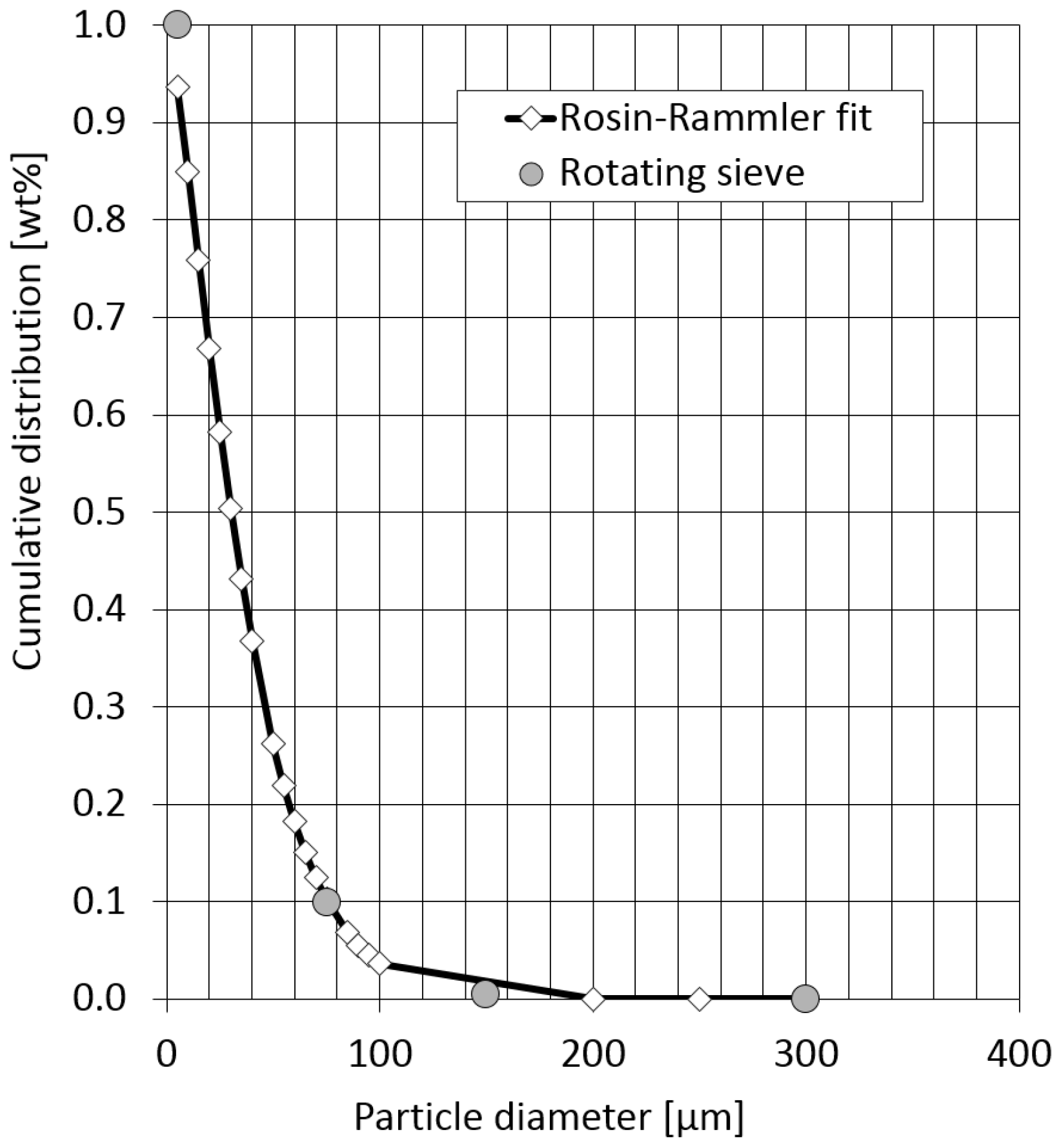
| Mean diameter | 40 | m | |
| Max diameter | 300 | m | |
| Min diameter | 5 | m | |
| Spread parameter | n | 1.31 | - |
| Number of classes | N | 10 | - |
| Coal Origin | Vitrinite % | Inertinite % | Liptinite % |
|---|---|---|---|
| Kleinkopje [59] | 35.4 | 62.3 | 2.3 |
| Highveld [60] | 11.2 | 87.7 | 1.1 |
| Coal Origin | C | H | O | N | S |
|---|---|---|---|---|---|
| Kleinkopje (Lab analysis) | 83.77 | 4.49 | 9.31 | 1.89 | 0.53 |
| Highveld [60] | 83.72 | 4.53 | 8.9 | 1.97 | 1.99 |
| Coal Origin | Ash | Volatile | Fixed Carbon |
|---|---|---|---|
| Kleinkopje (Lab analysis) | 13.97 | 24.46 | 61.57 |
| Highveld [60] | 28.11 | 24.44 | 47.45 |
| Parameter | Symbol | Value | Unit |
|---|---|---|---|
| Initial fraction of bridges in the coal lattice [56] | 0.83 | - | |
| Initial fraction of char bridges [56] | 0 | - | |
| Lattice coordination number [56] | 5.2 | - | |
| Cluster molecular weight [56] | 308 | kg/kmol | |
| Side chain molecular weight [55] | 30 | kg/kmol |
| Parameter | Symbol | Value | Unit |
|---|---|---|---|
| Mass Diffusion-Limited Rate Constant | - | ||
| Kinetic-Limited Rate Pre-Exponential Factor | 6.7 | - | |
| Kinetic-Limited Rate Activation Energy | J/kmol |
| Parameter | Symbol | Value | Unit |
|---|---|---|---|
| Mass Diffusion-Limited Rate Constant | - | ||
| Kinetic-Limited Rate Pre-Exp. Factor | 0.0302 | - | |
| Kinetic-Limited Rate Activ. Energy | J/kmol | ||
| Char porosity | 0.67 | - | |
| Mean pore radius | m | ||
| Specific internal surface area | 300,000 | m/kg | |
| Tortuosity | 1.4142 | - | |
| Burning mode | 0.2500 | - |
| Parameter | Symbol | Value | Unit |
|---|---|---|---|
| Coal density | 1300 | kg/m | |
| Coal specific heat | 1380 | J/(kgK) | |
| Low heating value | J/kg |
| Simulation | Devolatilization | Char Burnout |
|---|---|---|
| 1 | CPD | Int |
| 2 | CPD | KD |
| 3 | SKR | Int |
| 4 | SKR | KD |
| Parameter | Unit | CPD-Int | CPD-KD | SKR-Int | SKR-KD |
|---|---|---|---|---|---|
| Temperature | K | 1641 | 1674 | 1698 | 1715 |
| O mole fraction | - | 0.02973 | 0.02341 | 0.02828 | 0.02361 |
| CO mole fraction | - | 0.1548 | 0.1600 | 0.1560 | 0.1599 |
| HO mole fraction | - | 0.04944 | 0.05116 | 0.04981 | 0.05108 |
| NO concentration | ppm | 180.9 | 150.2 | 234.7 | 267.2 |
© 2017 by the authors; licensee MDPI, Basel, Switzerland. This article is an open access article distributed under the terms and conditions of the Creative Commons Attribution (CC-BY) license (http://creativecommons.org/licenses/by/4.0/).
Share and Cite
Torresi, M.; Fornarelli, F.; Fortunato, B.; Camporeale, S.M.; Saponaro, A. Assessment against Experiments of Devolatilization and Char Burnout Models for the Simulation of an Aerodynamically Staged Swirled Low-NOx Pulverized Coal Burner. Energies 2017, 10, 66. https://doi.org/10.3390/en10010066
Torresi M, Fornarelli F, Fortunato B, Camporeale SM, Saponaro A. Assessment against Experiments of Devolatilization and Char Burnout Models for the Simulation of an Aerodynamically Staged Swirled Low-NOx Pulverized Coal Burner. Energies. 2017; 10(1):66. https://doi.org/10.3390/en10010066
Chicago/Turabian StyleTorresi, Marco, Francesco Fornarelli, Bernardo Fortunato, Sergio Mario Camporeale, and Alessandro Saponaro. 2017. "Assessment against Experiments of Devolatilization and Char Burnout Models for the Simulation of an Aerodynamically Staged Swirled Low-NOx Pulverized Coal Burner" Energies 10, no. 1: 66. https://doi.org/10.3390/en10010066