Thermal Analysis of a Solar Powered Absorption Cooling System with Fully Mixed Thermal Storage at Startup

Abstract

A simple effect one stage ammonia-water absorption cooling system fueled by solar energy is analyzed. The considered system is composed by a parabolic trough collector concentrating solar energy into a tubular receiver for heating water. This is stored in a fully mixed thermal storage tank and used in the vapor generator of the absorption cooling system. Time dependent cooling load is considered for the air conditioning of a residential two-storey house. A parametric study is performed to analyze the operation stability of the cooling system with respect to solar collector and storage tank dimensions. The results emphasized that there is a specific storage tank dimension associated to a specific solar collector dimension that could ensure the longest continuous startup operation of the cooling system when constant mass flow rates inside the system are assumed.

1. Introduction

Absorption systems are widely studied as they are an eco-friendly alternative to conventional compression chillers. The energy input is waste heat or a renewable heat source, such as non-conventional solar or geothermal heat. Another benefit is that absorption units operate with environmental friendly working fluids. By combining the two mentioned advantages over mechanical compression cooling systems, one can achieve a reduction of the negative impact on the environment.

A detailed state of the art review of solar absorption refrigeration systems was published by Kalogirou [1]. Different analyses and numerical simulations have been performed by researchers in the field, leading to increased interest. Koroneos et al. [2] emphasized in their study that among all installed worldwide solar thermal assisted cooling systems, 69% are absorption cycle-based. Most of the published works on solar cooling systems are concentrated on absorption cycle systems operating with LiBr-H₂O solution and flat plate solar collectors. As Duffie and Beckman [3] emphasized, the temperature limitations of flat plate collectors imposed the use of LiBr-H₂O based systems. Ammonia-water based systems require higher temperature heat sources and thus are less used with flat plate collectors.

The potential of the ammonia–water absorption refrigeration system in Dhahran, Saudi Arabia, was evaluated by Khan et al. [4] for a cooling capacity of 10 kW driven by a 116 m² of evacuated tube solar collector. The system was coupled with dual storages of ice and chilled water used alternatively function on solar energy availability and in accordance with the cooling demands of a 132 m³ room.

A case study about converting an existing conventional ice-cream factory located in Isparta, Turkey to a solar energy based one is presented by Kizilkan et al. [5]. The authors proposed a system which involves the use of a parabolic trough solar collector instead of an existing electrically heated boiler. Also, instead of actual vapor compression refrigeration system, a H₂O-LiBr absorption refrigeration system is proposed for cooling the ice-cream mixtures. The authors found that the daily energy savings which can be achieved using the parabolic trough solar collector system are about 98.56%.

Lu and Wang [6] presented an experimental performance investigation and economic analysis of three solar cooling systems. The first system consisted of an evacuated tube U pipe solar collector driving a silica gel–water adsorption chiller; the second one was composed of a high efficiency compound parabolic concentrating solar collector connected to single-effect H₂O-LiBr absorption chillers; and the last one was made up of a medium temperature parabolic trough collector coupled to a double effect H₂O-LiBr absorption chiller. The results showed that the highest solar coefficient of performance (COP) was attained by the third system. The parabolic trough collector can drive the cooling chiller from 14:30 to 17:00 in an environment where the temperature is about 35 °C.

Ghaddar et al. [7] presented modelling and simulation of a H₂O-LiBr solar absorption system for Beirut. The results showed that the minimum collector area should be 23.3 m² per ton of refrigeration and the optimum water storage capacity should be 1000 to 1500 L in order to operate seven hours daily only on solar energy.

A comparison of three novel single-stage combined absorption cycles (NH₃/H₂O, NH₃/NaSCN and NH₃/LiNO₃) to the Goswami cycle was performed by Lopez-Villada et al. [8]. The studied cycles were driven by an evacuated tube collector, a linear Fresnel collector and a parabolic trough collector. The authors simulated the systems for a whole year in Sevilla, Spain, using TRNSYS software 2004 (Transient System Simulation Tool, developed by Solar Energy Laboratory, University of Wisconsin, Madison, WI, USA). They concluded that an evacuated tube collector is a more suitable solar technology for such systems.

Li et al. [9] investigated the experimental performance of a single-effect H₂O-LiBr absorption refrigeration system (of 23 kW refrigeration capacity) driven by a parabolic trough collector of aperture area 56 m² for air conditioning of a 102 m² meeting room located in Kunming, China, and analyzed appropriate methods for improving the cooling performance.

Another H₂O-LiBr solar driven system was presented by Mazloumi et al. [10] for a 120 m² room located in Iran, whose peak cooling load is 17.5 kW. The authors proposed a minimum parabolic trough collector area of 57.6 m² and associated hot water storage tank volume of 1.26 m³. The system operates between 6.49 h and 18.82 h (about 6 a.m. to 7 p.m.).

As one may notice, the study of H₂O-LiBr absorption refrigeration systems is widespread in the technical literature. Nevertheless, there are papers presenting comparisons between the operation of absorption systems using different working fluids. Among them, a comparison between NH₃-H₂O, H₂O-LiBr and other four mixtures is presented by Flores et al. [11]. When computing system performances, the authors found that H₂O-LiBr system has a small range of vapor temperature operation due to crystallization problems. Their study reports an operation generator temperature of about 75 °C–95 °C for H₂O-LiBr system, while for NH₃-H₂O system working under the same conditions, the range is higher, namely 78 °C–120 °C. The chosen working conditions were set to 40 °C condensation temperature, 10 °C vaporization temperature and 35 °C absorber one, while the cooling load was 1 kW. Key highlights of the above literature review are presented in

Table 1. Literature review data.

ACS Type	Cooling Load	Solar Collector	Storage Tank	Reference
NH3-H2O	10 kW (for a 132 m3 room), between 8:45 and 15:00	42 m2 ETC at 25° tilt, Saudi Arabia, clear sky in March, peak solar radiation 1000 W/m2, water, 900 L/h, 3 bar (80 °C)–6 bar(>100 °C), peak generator temperature 120 °C 32% collector efficiency	No hot thermal storage between collector and ACS, ice cold storage	[4]
H2O-LiBr	40 kW, ice-cream factory, between 12:00 and 15:00	143.63 m2 PTC (42.12 m × 3.5 m), 55.19 kW, Turkey, 500 W/m2 constant solar radiation, therminol-VP1 oil (25–212.7 °C at 3.9 bar), 87 °C constant generator temperature	No hot thermal storage between collector and ACS	[5]
H2O-LiBr simple effect	16 °C chilled water, Between 10:00 and 16:00 (6 h in sunny days)	CPC, 4 m2/kW cooling, China, Sunny day water, 0.02 kg/(sm2) 80–125 °C outlet water temperature 50% collector efficiency(125 °C)	Hot water tank (no data)	[6]
H2O-LiBr double effect	16 °C chilled water, Between 14:30 and 17:00 (2.5 h in sunny days)	80 m2 PTC (2 m2/kW cooling), 40 concentrating ratio, China, sunny day, tracking, 125–150 °C outlet water or oil temperature 44% collector efficiency (150 °C)	Hot water tank (no data)	[6]
H2O-LiBr	10.5 kW (for a 150 m2 house), 7 h/day	23.3 m2/TR 1 FPC at 15° tilt (80.6 m2 optimum), Beirut, water, 7 m3/h optimum, 50–85 °C generator temperature	Hot water tank 1300 L optimum (13–19 L/m2 collector)	[7]
NH3-H2O (compared to others)	175 kW peak, chilled water from 12 to 7 °C	600 m2 ETC (3.05 m2 aperture) and Fresnel (3.39 m2 aperture) at 20° tilt, PTC (5.39 m2 aperture) at 0° tilt, Spain, optimum temperature 90–120 °C (ETC is the best choice for NH3-H2O cycle)	Hot water tank 36 m3	[8]
H2O-LiBr	23 kW (for a 102 m2 room)	56 m2 PTC (26 m × 2.5 m), China Water, 0.602 kg/s 35%–45% collector efficiency (clear sky)	Hot water tank 1 m3	[9]
H2O-LiBr	17.5 kW peak (120 m2 room), between 9 and 19	57.6 m2 PTC (2 m wide), Iran Water preheated at 71 °C, 1800 kg/h max 92 °C storage tank water temperature	Hot water tank 1.26 m3	[10]
H2O-LiBr	1 kW	75–95 °C desorber temperature	-	[11]
NH3-H2O		78–120 °C desorber temperature	-

¹ TR = tone of refrigeration, 3.51 kW.

.

Concluding the above literature study, better performances are reported for H₂O-LiBr systems in comparison to NH₃-H₂O ones in air conditioning applications, but they operate in a lower and narrower range of vapor generator temperatures, due to the fluid’s risk of crystallization, thus NH₃-H₂O mixtures might still be good candidates for solar absorption cooling.

Complementary to the above published results, the present paper presents a thermodynamic analysis of a system composed of a parabolic trough collector, a solar tubular receiver, a fully mixed storage tank and a simple effect one stage NH₃-H₂O absorption cooling system. Time dependent cooling load is considered for a residential building occupied by four persons, two adults and two students [12]. The minimum necessary dimensions of the parabolic trough collector (PTC) and storage tank are determined in order to cover the whole day cooling load. Under these conditions, the objective of the work is to simulate daily operation for the whole system in July, in Bucharest (44.25° N latitude) and to emphasize the sensitivity of the operation stability to storage tank and PTC dimensions. Variation of the storage tank water temperature is represented along the entire day, under the considered variable cooling load, putting into evidence the turn on and turn off timings and thus the possible operation interval of the system.

2. Considered Cooling Load

The proposed system is designed to cover the cooling load of a residential building located in Bucharest (Romania). The house is composed by two storeys, having a living surface of 73.65 m² on the ground-floor and 59.05 m² on the first-floor. The walls are made of autoclaved aerated concrete brickwork, insulated with 10 cm polystyrene at the exterior side. Thermo-insulated and double glazed windows are considered. The global heat transfer coefficient U was computed for each building element (wall, door, floor, ceiling, window, etc.) considering conduction through the element structure and either interior and exterior convection for exterior elements, or twice interior convection for interior elements. Thickness and thermal conductivity for the layers of the wall structure are detailed in paper [12], interior convection heat transfer coefficient was considered 8 W·m⁻²·K⁻¹ for walls and 5.8 W·m⁻²·K⁻¹ for ceilings, while the exterior one was 17.5 W·m⁻²·K⁻¹. These values were chosen in accordance with Romanian norms [13]. The corresponding computed values for the global heat transfer coefficient are presented in

Table 2. Overall heat transfer coefficient values for building elements.

Building Element	U (W/(m2·K))
Exterior wall	0.298
Interior wall	0.887
Exterior and interior doors	2.32
Exterior windows	2.564
Ground floor	3.000
Ceiling above the ground floor	2.182
Mansard ceiling	0.371

.

The occupants are a family of four, two adults and two students, performing ordinary daily activities. The cooling load was computed summing up all external and internal loads, namely all heat rates exchanged between the building and ambient, all sensible and latent heat rates corresponding to perspiration and exhalation of occupants, humidity sources, electronic equipment, appliances and artificial lightening. Thermal inertia of the walls was considered. Also, the external heat rate was computed taking into account each wall orientation with respect to the Sun, and accordingly the time-dependent solar radiation reaching each vertical wall under clear sky conditions. More details about these calculations are given in [12].

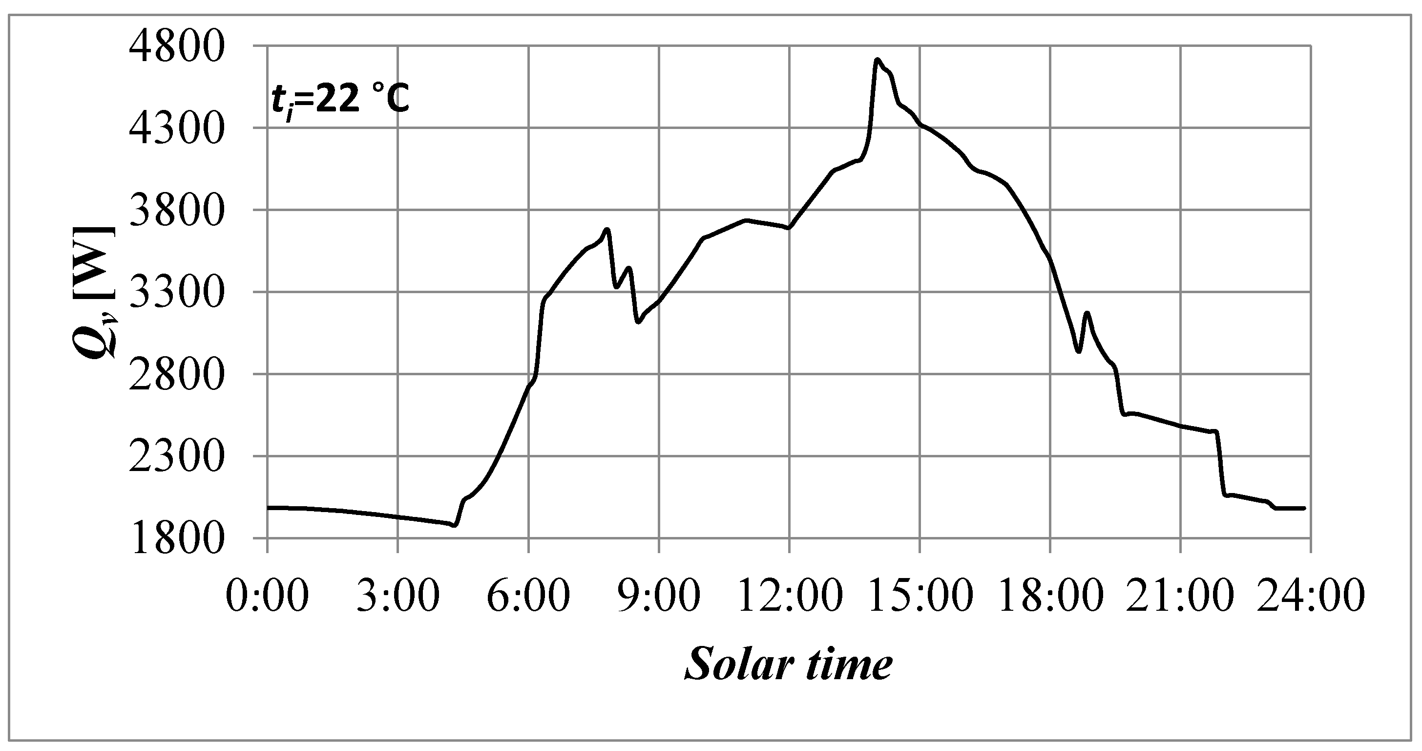
The time variation of this load on 15 July for an interior desired temperature of 22 °C, is presented in Figure 1. Note that this temperature value belongs to the lower part of the acceptable range of operative temperatures recommended by ASHRAE Standard [14] for residential buildings.

As one can notice, three peaks are apparent for the cooling load, around 8:00, 14:00 and 19:00, respectively. They are caused by the internal load contribution corresponding to occupants’ activity hours inside the building. The step downwards in the evening, around 22:00, corresponds to the moment when occupants are suspending their activity. The cooling load records a daily minimum around 5:00 and a daily maximum of 4709 W around 14:00.

In the present work, a cooling period between 9:00 and 18:00 will be considered. When the cooling system is considered off, the temperature inside the room is computed from the energy balance equations considering incoming solar energy when available, occupants’ activity and losses to or gains from the ambient. Obviously it differs from the set temperature of 22 °C. Thus, when the cooling system is turned on, the initial temperatures for building elements are those computed at that time. Consequently, in an indirect manner, the extra cooling loads not covered by the cooling system are considered by means of increased initial temperatures and building thermal inertia.

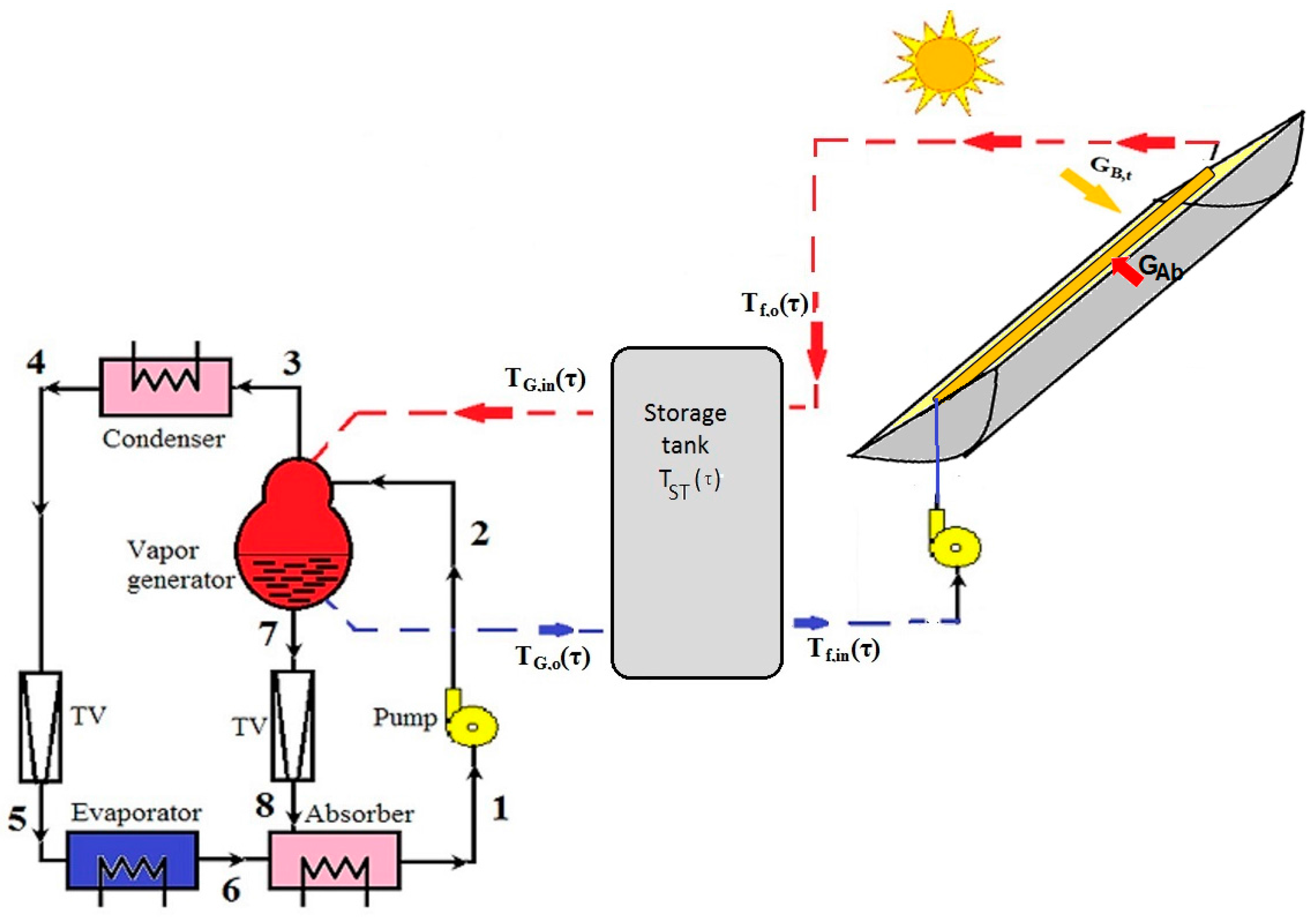
3. Description of the System

The considered solar driven system is shown in Figure 2. A parabolic trough collector (PTC) with a tubular receiver is used to catch solar radiation for heating the desorber of an absorption cooling system. Typical dimensions are between 1 to 3 m for aperture width and 2 to 10 m for its length, as reported by Fernandez-Garcia et al. [15] for solar-driven cooling applications. A single trough of 2.9 m by 10 m dimensions is expected to be used in the studied case. The collector is considered oriented fixed on an East-West direction, facing South and tilted at a fixed angle of 30° all day. These fixed collector constraints have the advantage of avoiding moving parts inside the system allowing lower acquisition and operating costs for this small-scale application. Also, for the considered latitude, the East-West orientation of the PTC provides an energy availability 6% lower with respect to a North-South orientation, as reported by Sharma et al. [16]. Nevertheless, it is here preferred since it offers a higher mechanical stability of the structure during windy days. Regarding the fixed tilt, its value was chosen so that maximum beam radiation is intercepted by the aperture plane around noon [17].

Inside the tubular receiver, liquid water is used as a heat career. The trend is to reduce operating costs. In this regard, one of the options is to employ a fluid that can be used for both heat collection and as a thermal storage medium [18]. According to technical literature regarding the operation of PTC, water can be used as working fluid for temperatures up to 220 °C; in this case the reported operating pressure is 10 kgf/cm² (9.8 bar); a pressurized expansion tank is used to maintain the pressure of circulating water in the closed system, allowing water to expand with rising temperature [19]. Nitrogen is used to regulate pressure variations. The disadvantage of using water as a working fluid is that a high pressure hot water storage tank must be employed and special safety precautions should be considered. A regularly monitor pressure should be mounted and safety relief valves should be set only by trained personal. Also the system should be enhanced by sensors to automatically defocus the trough from its position in case the water temperature exceeds the maximum allowable limit of 220 °C [19]. A heavy-duty quality steel tank should be used. Commercial ones are made of austenitic stainless steel 304, 316, 316 L or 316 Ti, as reported by manufacturers [20].

The water enters the receiver tube at temperature T_fi and exits at a superior temperature T_fo, as effect of the absorbed solar radiation. When exiting the receiver, the hot water enters a storage tank (ST).

After fully mixing with the existing water, a certain mass flow rate of ST water leaves the tank and heats the ammonia-water solution inside the vapor generator (at state 2 of temperature T_G,in, in Figure 2) of a classical one stage absorption cooling system (ACS). By “classical” one means a basic configuration for the system to operate: absorber, desorber (vapor generator), condenser, evaporator, throttling valves, liquid pump and all necessary connection devices. As a result of the heat exchange process in the desorber, first ammonia vapors leave the vapor generator at state 3 and fuel the refrigerating part of the absorption system, creating the cooling effect in the evaporator. The remaining solution, lean in ammonia, leaves the vapor generator at state 7, passes through the throttling valve and enters the absorber where it mixes again with the ammonia vapors leaving the evaporator (at state 6). The mass flow rate of water leaving the vapor generator and returning to the storage tank has now a lower temperature T_G,o.

4. Thermodynamic Modeling of the System

The thermodynamic model consists in applying the First Law of Thermodynamics for the whole system and system components. Conduction, convection and radiation heat exchange laws complete the system of equations. The mathematical model is presented for each computing stage, namely:

• the parabolic trough collector (PTC);
• the fully mixed storage tank (ST);
• the absorption cooling system (ACS).

The following general assumptions are made for the present study:

• clear sky conditions are assumed for the ambient and solar radiation data;
• time dependent cooling load (see Figure 1) is applied;
• thermal inertia of ACS and PTC is negligible with respect to that of the storage tank. As a result, unsteady model is considered only for the storage system. All other components of the system are modeled in steady state conditions;
• a fully mixed storage tank is considered. As a result, at each time T_G,in = T_f,in = T_ST.

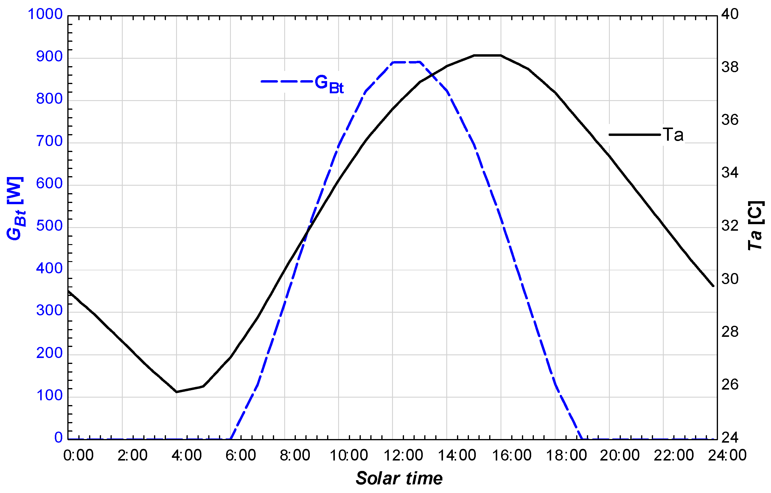
4.1. Solar Radiation and Ambient Data

Time averaged measured data between 1991 and 2010 for solar radiation and between 2000 and 2009 for ambient temperature are generated with Meteonorm V7.1.8.29631 software [21] for the Otopeni meteorological station (close to Bucharest). The data were extracted for 15 July with a time step of 10 min for clear sky conditions. The time variations of beam radiation on the PTC tilt surface, G_Bt, and ambient temperature, T_a, are shown in Figure 3. In the model, a wind speed w of 0.2 m/s was considered constant during the entire operating day.

4.2. Parabolic Trough Collector and Tubular Receiver Model

The parabolic trough collector is characterized by an opening of width H_PTC and a length L_PTC.

Its effective optical efficiency is computed as η_{env =} η_optK_θ. The term η_opt takes into account the optical losses for normal solar incident irradiance. These losses are due to receiver shadowing, tracking and geometry errors, dirt on the collector mirror and receiver, mirror reflectance, etc. In this paper a common value of 0.80 was adopted [22]. The incident angle modifier K_θ counts for the losses when solar irradiance is not normal to collector aperture. It takes into account the incidence losses, end shadowing of the through, reflection and refraction losses, etc. The incidence angle modifier was computed according to [23]:

$${\dot{Q}}_{in,R}={\eta }_{env}{H}_{\mathrm{PTC}}{L}_{\mathrm{PTC}}{G}_B={\eta }_{opt}{H}_{\mathrm{PTC}}{L}_{\mathrm{PTC}}{G}_{Bt}$$

(1)

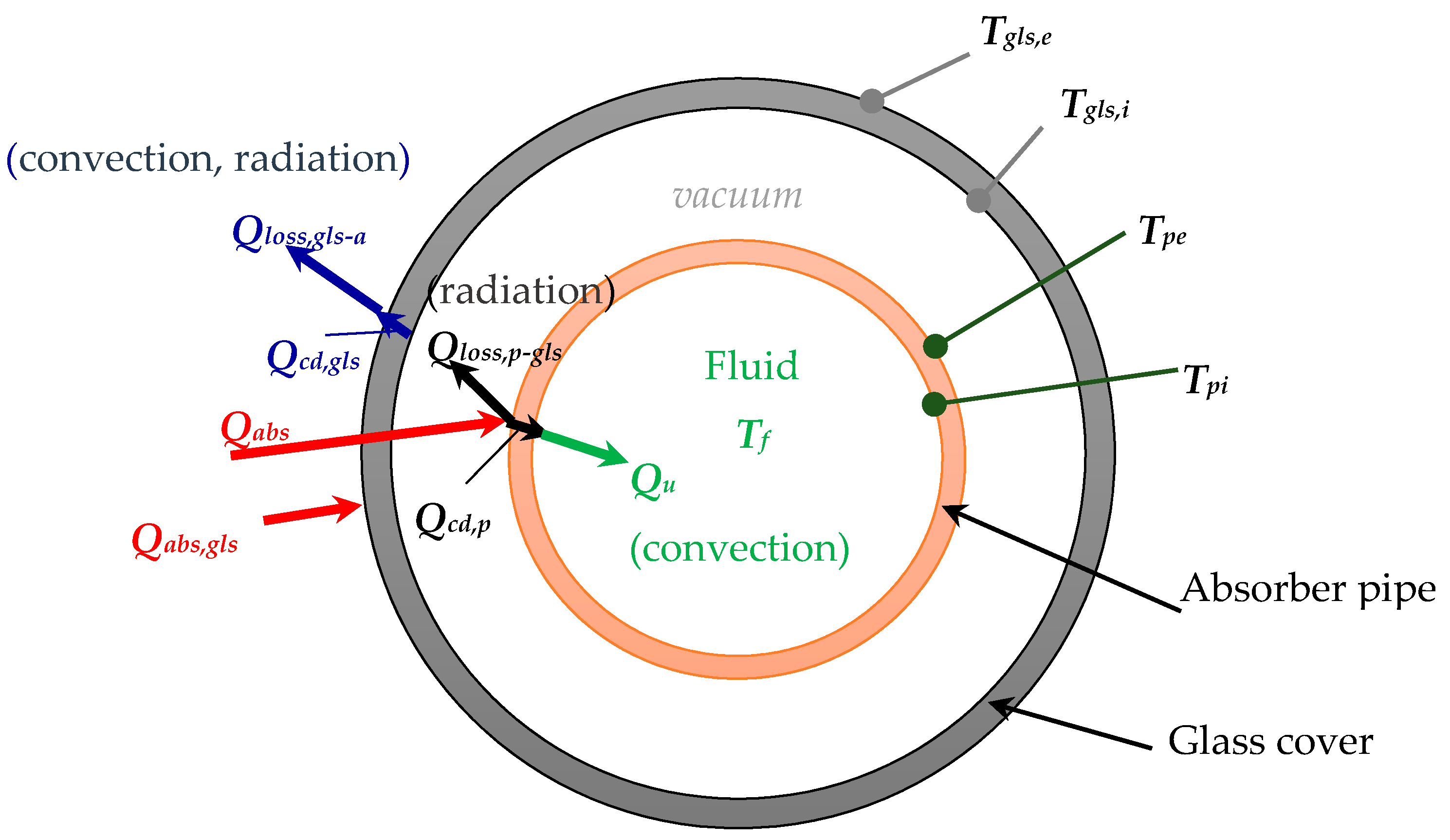
This heat rate is partially transmitted through the glass, absorbed by the pipe and so used to heat the fluid inside the receiver tube; the rest is lost by glass absorption, convection, conduction and radiation heat rates to ambient, as shown in Figure 4. In order to compute all heat rates, the geometry and characteristics of the tubular receiver should be firstly defined.

The tubular receiver is composed of a stainless steel pipe covered by a tubular Pyrex glass cover and has the following dimensions: pipe interior diameter D_pi = 0.051 m, pipe wall thickness of 0.001 m, tubular glass cover interior diameter D_gls,i = 0.075 m with a thickness of 0.001 m. The mass flow rate of fluid inside the tube, ${\dot{m}}_R$, is fixed to a value of 0.1 kg/s in order to maintain a laminar flow. The following glass properties are used: absorptivity α_gls = 0.02, emissivity ε_gls = 0.86, transmittance τ_gls = 0.935. For the stainless steel, the absorptivity is α_p = 0.92 and the emissivity is dependent on mean inside wall pipe temperature T_pi as: ε_p = 0.000327·T_pi − 0.065971 [22].

The mathematical model of PTC relies on the energy balance equations written on the inner and outer surfaces of absorber pipe and glass cover respectively. According to assumption iii these equations are written in steady state.

The absorbed heat rate by the absorber pipe is computed as:

$${\dot{Q}}_{abs,p}={\tau }_{gls}{\alpha }_p{\dot{Q}}_{in,R}$$

(2)

The useful part of ${\dot{Q}}_{abs,p}$ is transmitted through the pipe by conduction and then by convection to the fluid. Thus, the energy balance equation written on the inner pipe surface looks like:

$${\dot{Q}}_u={\dot{Q}}_{cd,p}$$

(3)

where the conduction heat rate through the tubular pipe is:

$${\dot{Q}}_{cd,p}=2\pi L_{\mathrm{PTC}}{\lambda }_p\frac{T_{pe}-T_{pi}}{\ln \frac{D_{pe}}{D_{pi}}}$$

(4)

The fluid receives this heat rate by thermal convection:

$${\dot{Q}}_u=\pi D_{pi}{L}_{\mathrm{PTC}}{h}_f\left(T_{pi}-T_f\right)$$

(5)

where T_f is the mean temperature of the water flowing inside the absorber pipe. Since the heat transfer is developing under constant heat flux boundary condition, one may consider that T_f is the arithmetic mean temperature between inlet and outlet temperatures T_fi and T_fo.

The convection heat transfer coefficient h_f is computed from Nusselt number considered 4.36 as the flow inside the tube is kept laminar:

$$h_f=\frac{N{u}_f{\lambda }_f}{D_{pi}}$$

(6)

On the other hand, the useful heat rate received by the fluid can also be written as:

$${\dot{Q}}_u={\dot{m}}_f{c}_{p,f}\left(T_{fo}-T_{fi}\right)$$

(7)

At each time step, the inlet fluid temperature T_fi is equal to the storage tank fluid temperature, T_ST, as the fluid is recirculated from the storage tank through the PTC.

The energy balance equation on the pipe exterior surface is:

$${\dot{Q}}_{abs,p}={\dot{Q}}_u+{\dot{Q}}_{loss,p-gls}$$

(8)

where ${\dot{Q}}_{abs,p}$is computed by Equation (2) and ${\dot{Q}}_{loss,p-gls}$ represents lost heat rate between the pipe and glass cover. A common assumption is to consider vacuum inside this enclosure so that convection is neglected. Thus, ${\dot{Q}}_{loss,p-gls}$ is entirely due to radiation losses between pipe and glass cover:

$${\dot{Q}}_{loss,p-gls}=\pi D_{pe}{L}_{PTC}\sigma \frac{T_{pe}^4-T_{gls,i}^4}{\frac{1}{{\epsilon }_p}+\frac{1-{\epsilon }_{gls}}{{\epsilon }_{gls}}\frac{D_{pe}}{D_{gls,i}}}$$

(9)

where σ is the Stefann-Boltzman constant.

Further, the energy balance equation on the inner surface of the glass cover is:

$${\dot{Q}}_{loss,p-gls}={\dot{Q}}_{cd,gls}$$

(10)

where:

$${\dot{Q}}_{cd,gls}=2\pi L_{\mathrm{PTC}}{\lambda }_{gls}\frac{T_{gls,i}-T_{gls,e}}{\ln \frac{D_{gls,e}}{D_{gls,i}}}$$

(11)

represents the heat rate passing through the glass cover by conduction. The glass conductivity λ_gls corresponds to the mean of the inner and outer surface temperatures of glass cover.

Finally, the energy balance equation on the outer surface of glass cover is:

$${\dot{Q}}_{cd,gls}+{\dot{Q}}_{abs,gls}={\dot{Q}}_{loss,gls-a}$$

(12)

The heat flux absorbed by the glass cover is expressed by:

$${\dot{Q}}_{abs,gls}={\alpha }_{gls}{\dot{Q}}_{in,R}$$

(13)

The loss heat rate, ${\dot{Q}}_{loss,gls-a}$is transmitted from the outer glass surface to ambient through wind convection and radiation so that:

$${\dot{Q}}_{loss,gls-a}=\pi D_{gls,e}{L}_{\mathrm{PTC}}{h}_w\left(T_{gls,e}-T_a\right)+\pi D_{gls,e}{L}_{\mathrm{PTC}}{\epsilon }_{gls}\sigma \left(T_{gls,e}^4-T_{sky}^4\right)$$

(14)

The wind convection heat transfer coefficient is computed according to [24]:

$$h_w=5.7+3.8w$$

(15)

The set of equations is now completely defined so that solving of unknown temperatures T_pi, T_pe, T_gls,i, T_gls,e, T_fo may proceed. The outlet fluid temperature determined from Equation (7) is now a data input to the storage tank module.

4.3. Fully Mixed Storage Tank Model

A 0.16 m³ storage tank is considered for which a constant heat loss coefficient is assumed, ${\left(UA\right)}_{ST}$ = 11 W/K [3]. As pointed out above, the temperature inside the storage tank, T_ST, is assumed to be uniformly distributed. By using the mathematical expression of the First Law, one obtains the following ordinary differential equation:

$${\left(m{c}_p\right)}_{ST}\frac{d{T}_{ST}}{d\tau }={\dot{Q}}_u-{\dot{Q}}_G-{\left(UA\right)}_{ST}\left(T_{ST}-T_a\right)$$

(16)

The right hand side in Equation (16) counts for all heat rates exchanged by the storage tank with the exterior: the useful heat flux, ${\dot{Q}}_u$, received by the water inside the absorber pipe of PTC is computed by Equation (7), ${\dot{Q}}_G$ is the heat rate transferred from the storage tank to the vapor generator of the ACS, while the last term counts for heat flux losses to the ambient. Since all the above heat fluxes depend on time, one cannot develop an analytical solution for this equation. Thus, a first order explicit discretization with respect to time is employed, which leads to the discrete relation:

$$T_{ST}^{(n+1)}=T_{ST}^{(n)}+\frac{{\dot{Q}}_u^{(n)}-{\dot{Q}}_G^{(n)}-{\left(UA\right)}_{ST}\left(T_{ST}^{(n)}-T_a^{(n)}\right)}{{\left(m{c}_p\right)}_{ST}}\Delta \tau$$

(17)

where superscript (n + 1) denotes the properties values at time τ + Δτ and subscript (n) identifies the values of properties at current time τ.

4.4. Absorption Cooling System Model

For the operation of the considered NH₃-H₂O absorption cooling system, the vaporization temperature is imposed at t_v = 10 °C and the above described cooling load ${\dot{Q}}_v$ is applied.

The condenser and absorber are cooled with ambient air, so that condensation temperature T_c as well as the absorber temperature T_Ab are imposed by T_a, time dependent. The heat source required to feed the desorber is the hot water from the storage tank at T_ST. Thus the solution temperature at the end of desorbing process is constrained by this value.

According to assumption iii, steady state operation is assumed. The transient response of the ACS module is negligible in comparison to that of the storage tank. Due to this hypothesis, one expects that the obtained results would be overestimated before the storage tank water temperature reaches its maximum value and underestimated afterwards. Further, neglecting the variation of kinetic and potential energies (which is an appropriate assumption for the studied system), the First Law of Thermodynamics becomes:

$$\dot{Q}-\dot{W}={\displaystyle \sum _o{\left(\dot{m}h\right)}_o-{\displaystyle \sum _i{\left(\dot{m}h\right)}_i}}$$

(18)

which is applied to each component of the system.

The energetic and exergetic analyses are detailed in previous works [25]. The set of equations is summarized in

Table 3. Heat rates in the ACS.

Component	Thermal Load	Component	Thermal Load
Condenser	${\dot{Q}}_C={\dot{m}}_0\left(h_4-h_3\right)$	Vapor Generator	${\dot{Q}}_G=\dot{m}\left(h_7-h_2\right)+{\dot{m}}_0\left(h_3-h_7\right)$
Evaporator	${\dot{Q}}_V={\dot{m}}_0\left(h_6-h_5\right)$	Absorber	${\dot{Q}}_{Ab}=\dot{m}\left(h_8-h_1\right)+{\dot{m}}_0\left(h_6-h_8\right)$

.

The overall coefficient of performance and exergetic efficiency are expressed by:

$$COP=\frac{{\dot{Q}}_V}{{\dot{Q}}_G+\left|{\dot{W}}_P\right|}$$

(19)

$${\eta }_{Ex}=\frac{{\dot{Q}}_V\left(\frac{T_a}{T_V}-1\right)}{{\dot{Q}}_G\left(1-\frac{T_a}{T_{Gm}}\right)+\left|{\dot{W}}_P\right|}$$

(20)

In the above relations, $\left|{\dot{W}}_P\right|$ represents the pump consumed power and T_Gm is a mean value for the generator temperature, defined as arithmetic mean between temperature values of the states corresponding to the beginning and ending of the desorbing process.

5. Operating Regimes of the System

Depending on solar radiation availability, the cooling time interval and the correct operation conditions of ACS, the following possible operating regimes of the system can occur:

(i)

During night and early morning, the solar radiation is not available, so that the PTC module is inactive and the water circulation through its pipes is stopped. In this case, only the storage tank module is computed and, due to losses to ambient, the fluid temperature T_ST decreases.

(ii)

As far as solar radiation is available, both PTC and ST modules are operating. The storage tank water temperature is increasing as a certain mass flow rate is circulated through the PTC pipes.

(iii)

At the targeted ACS starting time (9:00 in the studied case), the ACS module can start only if the storage tank water temperature is sufficiently high to ensure appropriate operating conditions in terms of concentration difference between strong and weak solutions (>0.06). Obviously this difference mainly depends on the ambient temperature too, as well as on the cooling load. If the condition is not satisfied, the ACS module is stopped. In this case, only the PTC and ST modules are working and the storage tank water temperature increases. When it reaches the necessary value to fulfill the above condition, the ACS module is started again.

As conclusion, one may find that the ST module is 24 h operating, the PTC module works as long as the solar beam radiation is available, while the ACS module may function either on its entire targeted period (i.e., 9:00–18:00), or on shorter inside intervals of time, as the appropriate operating conditions are fulfilled or not.

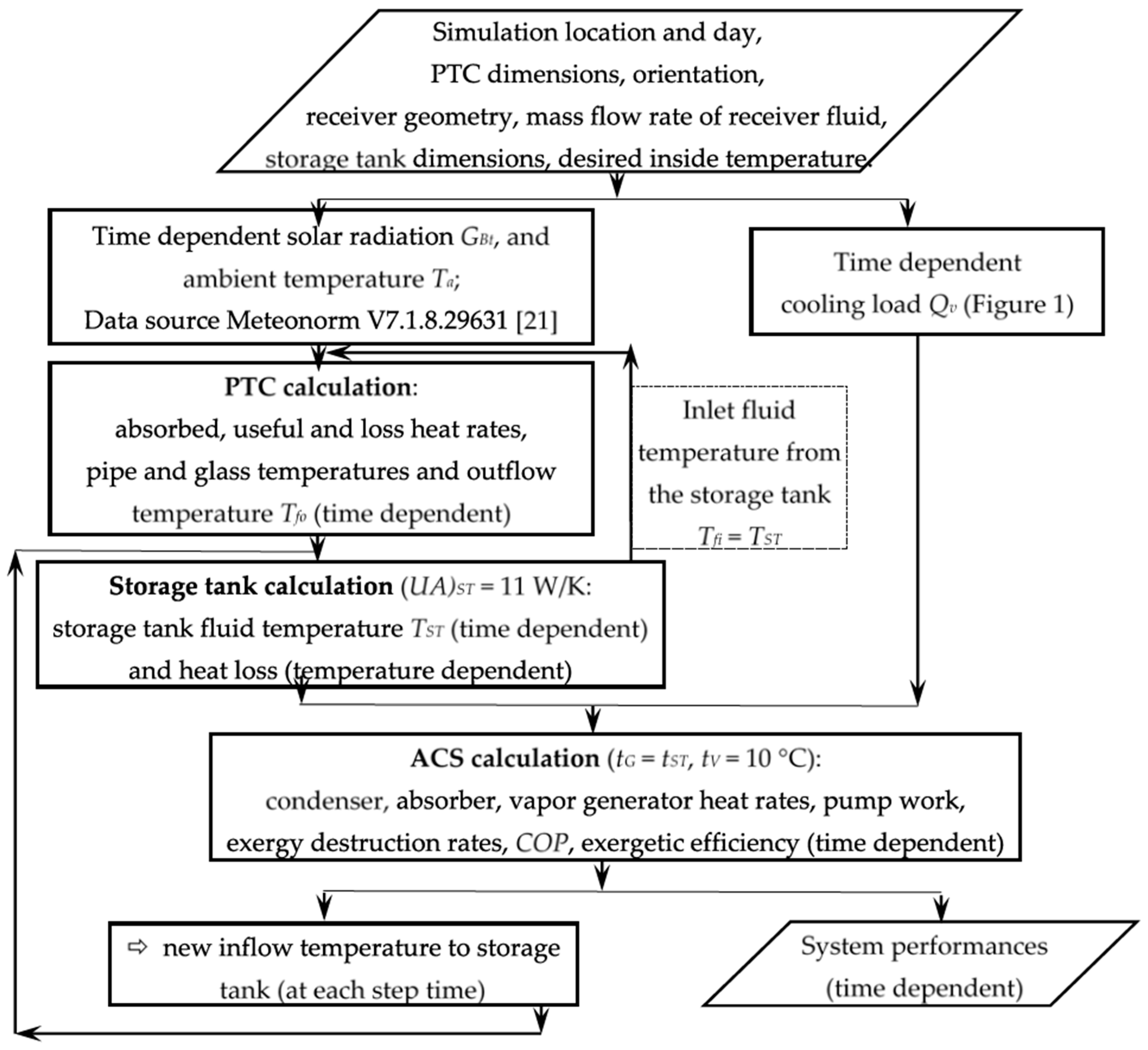
6. Numerical Procedure

The simulation of the entire system operation is worked out in EES programming environment [26], by following the algorithm presented in Figure 5. Firstly, the input data of the system are set. The cooling load demand data (see Figure 1) as well as the direct solar radiation and ambient temperature data (see Figure 3) were stored in lookup tables. All other geometrical parameters of the system were specified at the top of main code.

Three modules have been coded for modeling the working regimes of PTC, ACS and ST, respectively. At the current time-step calculation, the PTC module reads G_Bt and T_a data from the corresponding lookup tables and receives as input the fluid temperature T_fi from the storage tank. Then it solves the Equations (3), (8), (10) and (12). The output of this module is the fluid output temperature T_fo, further used as input in the storage tank module.

The ACS module checks the necessary operating conditions and if fulfilled, computes the performances of the cooling system according to Equations (19) and (20). The input data are the temperatures T_a and T_ST, as well as the cooling load ${\dot{Q}}_V$computed at the current time. The specific properties of the working fluid (ammonia-water pair) are determined by means of a dynamically linked procedure, in which the correlations proposed by Ibrahim and Klein [27] are used. The output in terms of outlet generator fluid temperature T_Go is sent to the storage tank module.

The ST module has as inputs the temperatures T_fo, T_Go and T_ST computed at the current time. Losses to the ambient are calculated and Equations (17) is employed to find the storage tank water temperature T_ST at the next time, τ + Δτ.

The main program calls these modules according to the operating regimes of the system presented in the previous section.

The computations are started at 00 a.m., 15 July. At this time, the water temperature in the storage tank was considered 10 °C higher than T_a. The time step was set to Δτ = 10 min, and was kept constant during the entire day.

7. Results and Discussions

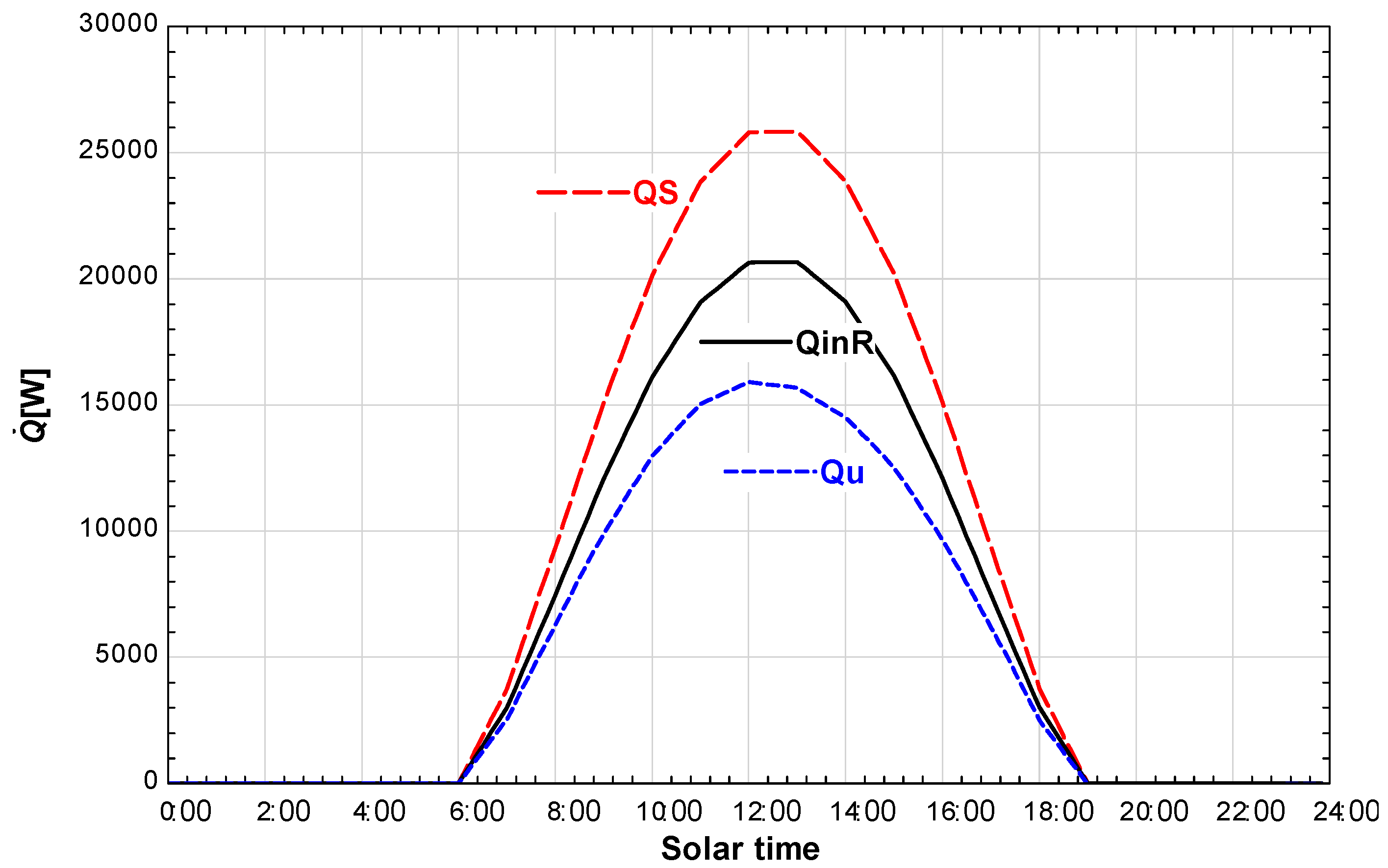
As pointed out before, a PTC of 2.9 m wide and 10 m long is considered. Available solar heat rate ${\dot{Q}}_S$, input heat rate to the tubular receiver ${\dot{Q}}_{in,R}$ and useful heat rate transmitted to the fluid ${\dot{Q}}_u$ are sketched in Figure 6. An important aspect to notice is that solar radiation is available between 6:00 and 19:00.

After some initial trials, the storage tank volume was set to 0.16 m³ in order to maintain the water temperature in the operation range of the cooling module as long as possible. For lower tank volumes, the water temperature increased too much in the morning while for higher values, the temperature was too low to cover the considered cooling load.

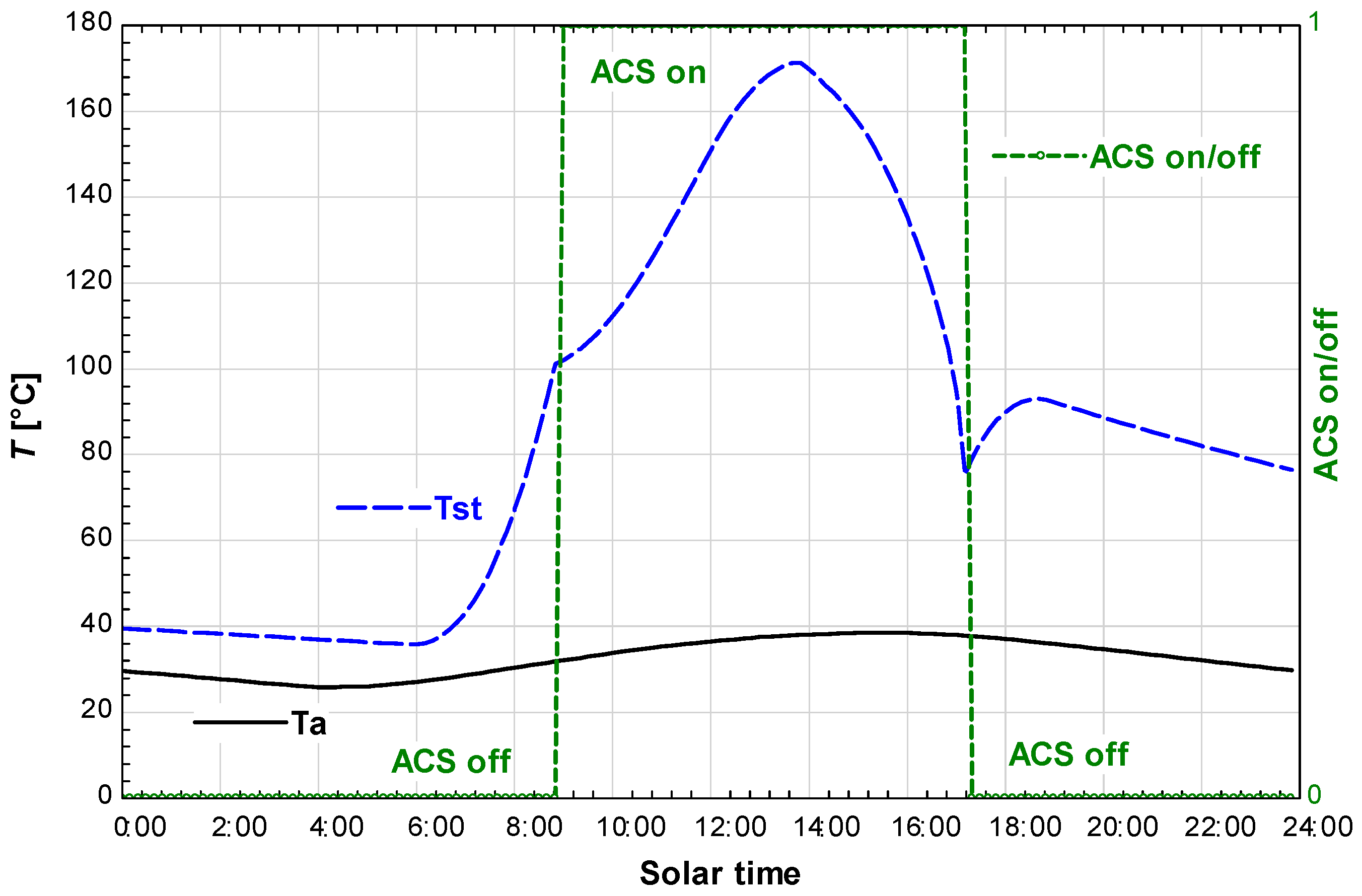
The starting time of the simulation is 00 a.m. The (i) operating regime described in Section 5 is applied. Till 6:00, the temperature of the fluid in the storage tank is slowly decreasing as heat is lost to the ambient. At 6:00 solar radiation starts reaching the PTC surface, so the water circulation through the PTC is started, corresponding to operation regime (ii). As a consequence, water temperature starts increasing as presented in Figure 7 by the dotted blue line T_ST. It raises from 38 °C at 6:00 to 100 °C at 9:00. At 9:00 the absorption cooling system (ACS) is started, so that water is now recirculated also through the desorber of the ACS, heating the NH₃-H₂O solution and assuring its operation for covering the cooling demand. Operating regime (iii) is applied. The storage tank water temperature is still increasing, but with a lower slope. This behavior is due to the following two effects: on one side the solar radiation reaching the PTC surface is increasing in intensity, on the other hand thermal energy of stored water is used in the ACS desorber.

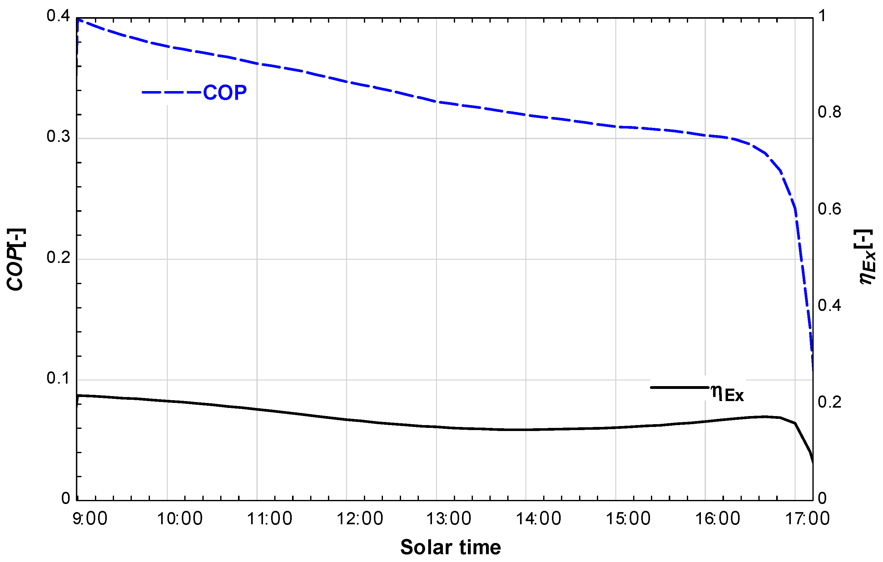
As one may see in Figure 8, the coefficient of performance of the ACS is slowly decreasing and also its exergetic efficiency. A minimum for the exergetic efficiency is met around 14:00. In fact, this value corresponds to the maximum value of the storage tank water temperature, encountered at 13:40. The operation of the ACS is very sensitive to the heat source temperature value, among other parameters. It was previously proved [27] that the exergetic efficiency of such a system has a maximum around a relatively low desorber temperature of about 80–90 °C and then it starts decreasing when increasing the desorber temperature. The same behavior is met here. As the desorber temperature increases, the exergetic efficiency of the ACS decreases. After this peak, the storage tank temperature drastically starts to decrease and when its value arrives to 75 °C the ACS operation is no more possible. This happens at 17:10. As a consequence of temperature decrease, the exergetic efficiency increases on this second working period (Figure 8).

After the ACS is stopped and thus no cooling load can be covered from the available heat source, the storage tank temperature begins to increase for the period of solar radiation availability, i.e., till 19:00. Operating regime (ii) is applied again. After 19:00, (i) operating regime is involved and water temperature slowly decreases due to losses to ambient.

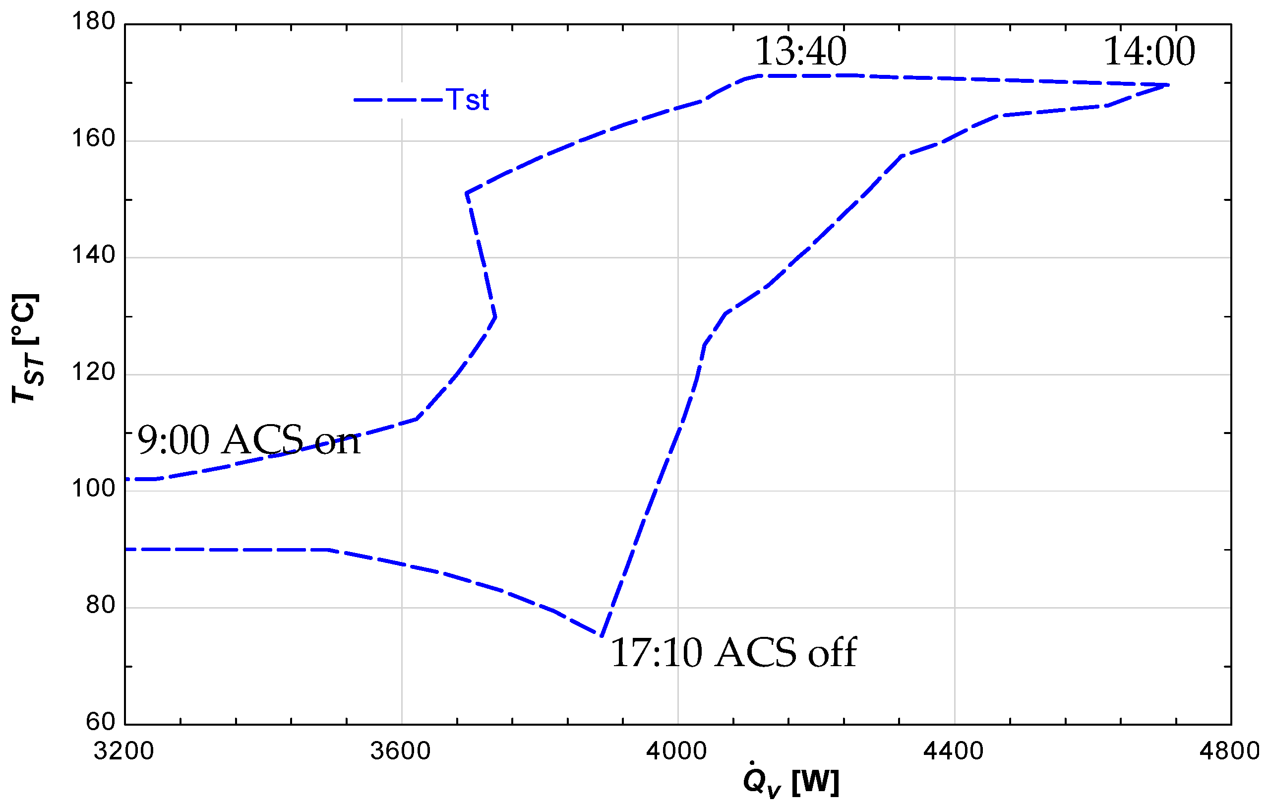
The sensitivity of the storage tank fluid temperature to the variation of the cooling load along the day may be analyzed in detail in Figure 9. One may now observe that the cooling load is covered continuously between 9:00 and 17:10. The storage tank temperature increases continuously up to 13:40. This means that even if the cooling load is increasing and “consuming” more heat from the storage tank (sending the fluid with a lower temperature back to the storage tank), the increase of solar radiation on this period is enough to cover this load. After 13:40 the storage tank temperature slowly decreases to 14:00 when the cooling demand peak is met, and then drastically decreases even if the cooling load is decreasing too. The solar radiation is no more sufficient to maintain T_ST above the operation limit so that at 17:10 the ACS is turned off.

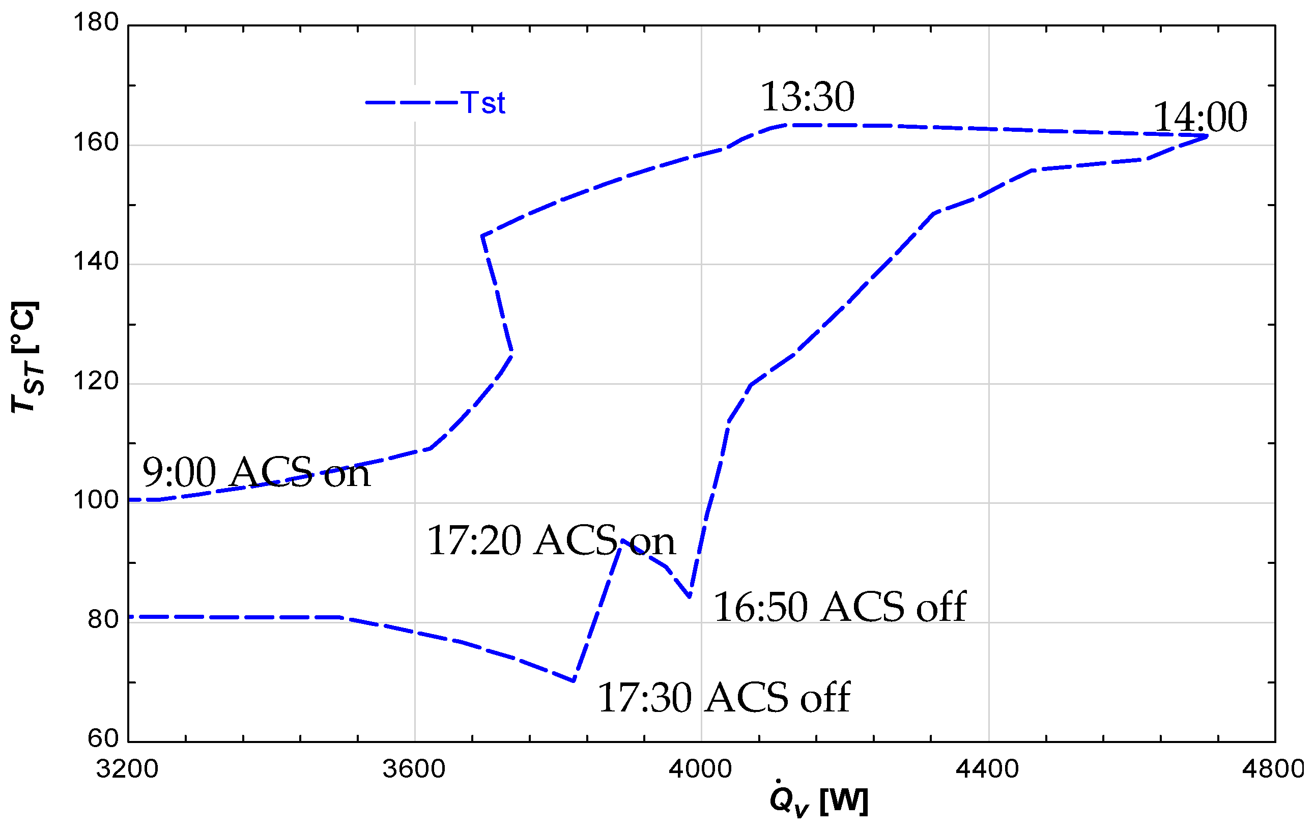
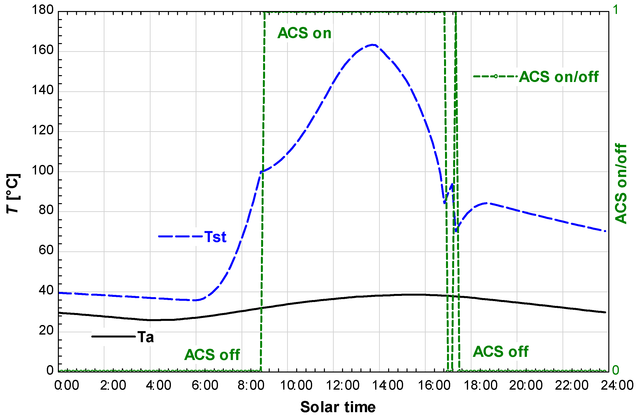
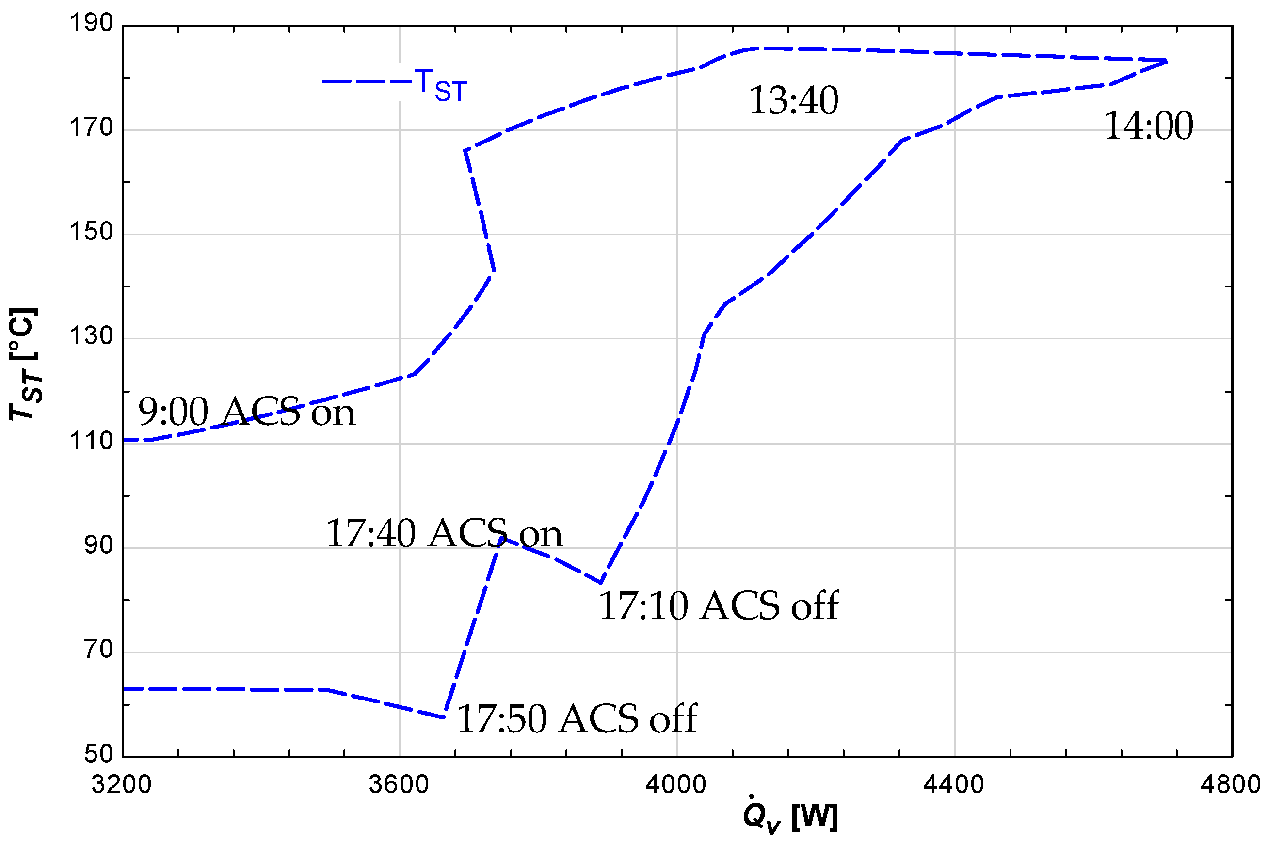
From the above results, one might think about possibilities for improving the operation of the global system. One of them is to reduce the storage tank temperature so that the exergetic efficiency of the ACS increases. Thus, a simulation was done considering exactly the same parameters except the length of the PTC which was reduced from 10 m to 9.8 m. In this case, the results emphasize a smaller value of the maximum storage tank temperature, but the ACS is turned off automatically earlier, at 16:50, since the desorber temperature has dropped to an insufficient value for the ACS operation (84 °C). As solar radiation is still available, storage tank temperature increases enough to turn on ACS at 17:20, but as it is not sufficiently high, 10 min after, the ACS is turned off again. This is shown in Figure 10 and Figure 11. This case emphasize the instability in ACS operation on the last part of the day. Obviously, such variations should be avoided.

Another improving solution would be to extend the ACS operation period by storing a higher quantity of thermal energy. This could be done by reducing the quantity of storage tank water. When doing a simulation with 0.14 m³ of water instead of 0.16 m³, a similar behavior as in the previous case was met. The storage tank temperature reached a higher maximum value (185 °C) in comparison to the previous two cases, but the temperature dropped rapidly so that at 17:10 the ACS was turned off, too. A second attempt of turning on was met at 17:40 but only for 10 min. Results are presented in Figure 12.

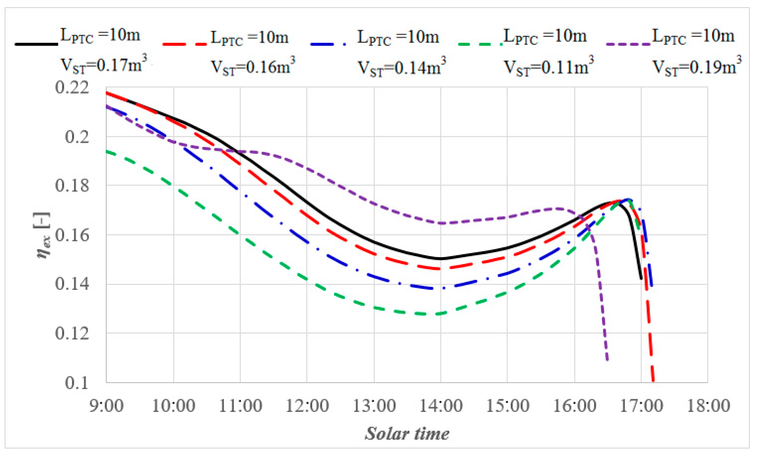
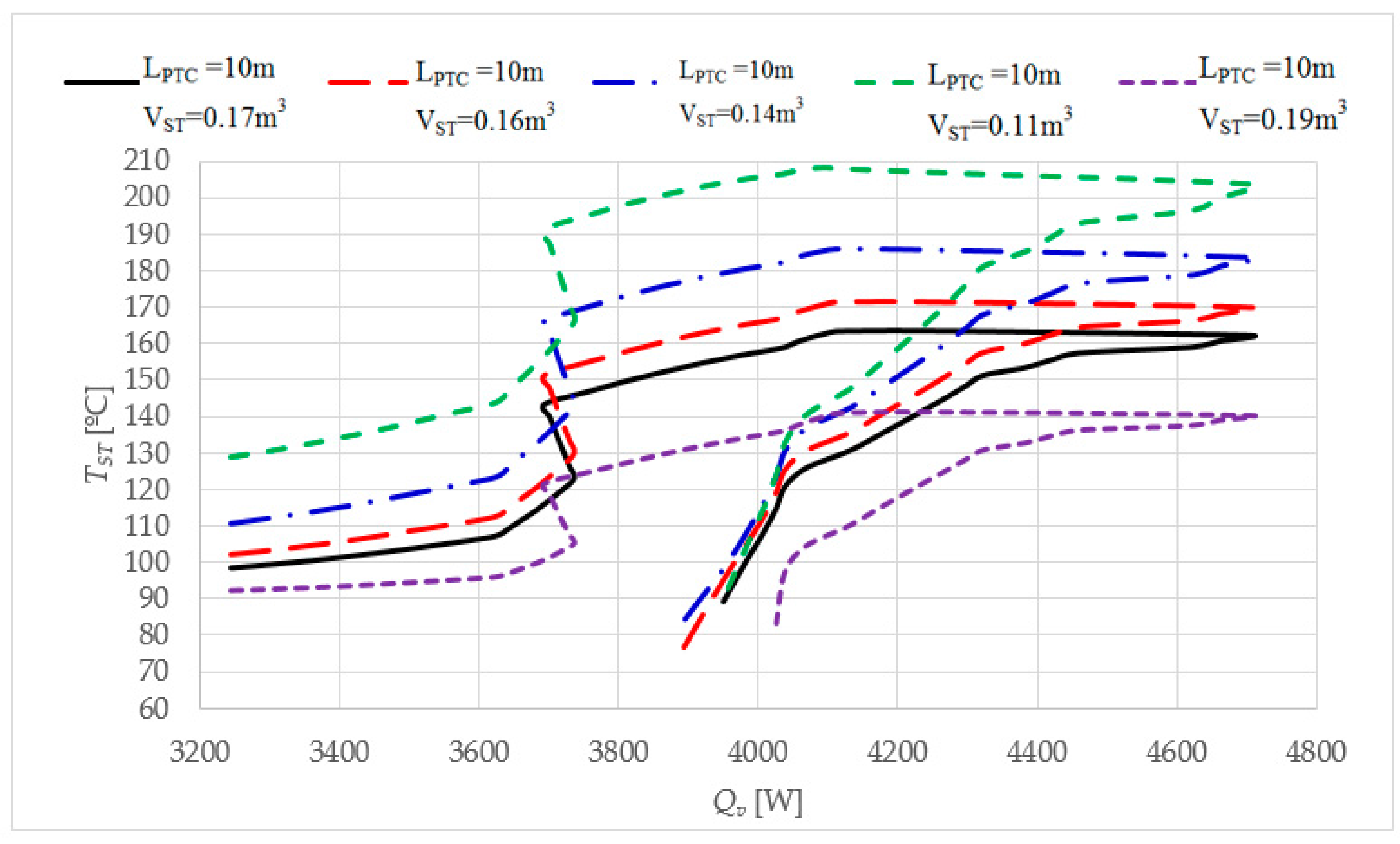
One may conclude that the ACS operation is very sensitive to storage tank temperature and consequently to design parameters. There should be a narrow range of PTC and storage tank dimensions that fits the ACS operation. In this regard, a sensitivity study with respect to storage tank dimensions for a given PTC length is emphasized in Figure 13 for the ACS exergetic efficiency and in Figure 14 for the dependence of the storage tank temperature on the cooling load.

One may see that the best ACS exergetic efficiency is obtained when the storage tank temperature is the lowest (the dotted magenta curve in Figure 13 and Figure 14, corresponding to 0.19 m³ storage tank). In this case, the cooling load is not entirely covered on the targeted period 9:00–17:00. The system is turned off at 16:30 as the storage tank water temperature dropped under the desorber operation level. Increasing more the storage tank dimension leads to a lower level of the storage tank water temperature along the day and the ACS operation cannot be covered at all at the required cooling load.

Another important aspect regards the optimum dimensions of the PTC-ST systems for continuous operation. There is a specific storage tank dimension associated to a specific PTC dimension that could ensure the longest possible operation with a good ACS exergetic efficiency (the red dotted curve corresponding to 10 m × 2.9 m PTC and 0.16 m³ water storage tank). The results emphasized the optimum dimensions of the solar collector and storage tank required for a fully solar startup of the system.

8. Conclusions

A solar driven NH₃-H₂O absorption cooling system was analyzed from the point of view of the best sizing of solar-storage part of the global system for the longest possible daily operation in July, at 44.25° N latitude. Measured meteorological data have been employed, generated by Meteonorm software. Cooling load was time dependent computed for a two storeys residential building. A fully mixed hot water storage tank was used to fuel the desorber of the cooling system from the heat collected by a fixed oriented parabolic trough collector. The results emphasized that there is a specific storage tank dimension associated to a specific PTC dimension that could ensure the longest continuous operation of the ACS when constant mass flow rates inside the system are assumed. An initial solar start-up was considered, meaning that the initial temperature of storage tank water was close to the ambient one. The longest continuous operation of the NH₃-H₂O cooling system (from 9 a.m. to 5:10 p.m.) was obtained for a 10 m × 2.9 m PTC aperture dimensions with a 0.16 m³ storage tank volume. The simulations emphasized that the ACS operation was very sensitive to these values. Any change in PTC or ST dimensions would diminish the operation time of the ACS.

From the best exergetic efficiency point of view, a 0.19 m³ storage tank capacity is preferred, and as a result, the ACS operation period is reduced by 40 min. Thus, different optima lead to different sets of PTC and ST dimensions.

Further analyses may be thought implementing a control-command unit for variable mass flow rates to the PTC and ACS system, regulating the desorber temperature as needed. A comparative analysis may be envisaged between this studied case and the corresponding fully solar startup with a previous stored thermal energy from an earlier operation of the PTC-ST modules alone.