A Mixed Logical Dynamical-Model Predictive Control (MLD-MPC) Energy Management Control Strategy for Plug-in Hybrid Electric Vehicles (PHEVs)

Abstract

Plug-in hybrid electric vehicles (PHEVs) can be considered as a hybrid system (HS) which includes the continuous state variable, discrete event, and operation constraint. Thus, a model predictive control (MPC) strategy for PHEVs based on the mixed logical dynamical (MLD) model and short-term vehicle speed prediction is proposed in this paper. Firstly, the mathematical model of the controlled PHEV is set-up to evaluate the energy consumption using the linearized models of core power components. Then, based on the recognition of driving intention and the past vehicle speed data, a nonlinear auto-regressive (NAR) neural network structure is designed to predict the vehicle speed for known driving profiles of city buses and the predicted vehicle speed is used to calculate the total required torque. Next, a MLD model is established with appropriate constraints for six possible driving modes. By solving the objective function with the Mixed Integer Linear Programming (MILP) algorithm, the optimal motor torque and the corresponding driving mode sequence within the speed prediction horizon can be obtained. Finally, the proposed energy control strategy shows substantial improvement in fuel economy in the simulation results.

1. Introduction

Focusing on plug-in hybrid electric vehicles (PHEVs), which are a typical hybrid system (HS) [1], an accurate system model is mandatory to study their control strategy. Commonly used hybrid system modeling methods include hierarchical model [2], Petri net model based on the proposed network diagram [3], the “unified model” of hybrid dynamic systems by Branicky et al. [4] and the Piecewise Affine (PWA) switching model [5]. All these models are relatively complex and inconvenient compared to the conventional control technology. In [6], Bemporad and Morari proposed the mixed logical dynamical (MLD) model that includes interdependent physical laws, logic rules and operational constraints, to apply the conventional control methods (e.g., optimization and prediction) to the hybrid system. The MLD model also uses differential equations to avoid the complex conditions in hybrid systems and could be transferred into mixed integer linear programming (MILP) [7] for a solution.

The control strategy for PHEVs aims to find an appropriate power and torque distribution between the combustion engine and the electric motor to improve the fuel economy and emission performance [8]. Among various control strategies, the rule-based control method [9] is the most widely used, but it relies on experience to a greater extent, which makes it difficult to adapt to dynamic changes in the driving cycles and to optimize the fuel economy of the vehicle. The optimization-based control strategy [10] includes instantaneous optimization and global optimization. The instantaneous optimization control strategy [11] for an equivalent minimal fuel consumption does not give sufficient consideration to the vehicle state in the future; while for the global optimization [12], complete statistical information on driving cycles must be provided, including road conditions, which makes it hard to compute fast and it lacks adaptability, and eventually cannot be applied directly to real-time control of the vehicle. If the vehicle state information is predicted accurately beforehand, global optimization within this time could be applied to overcome the disadvantages of inadaptability. This could also form the basis of the Model Predictive Control (MPC) method for a hybrid electric vehicle. In [13], a generalized predictive optimal control framework is proposed, and MILP methodology is utilized, which enables the control strategy to get better economy than instantaneous strategies. However, it assumes the traffic pattern and terrain are known in advance without any prediction.

In this paper, the required vehicle torque is calculated based on the predicted vehicle speed. Commonly used vehicle speed prediction methods are the model-based method [14], Kalman filter [15], hidden Markov models [16] and neural network models [17], etc. The non-linear auto-regressive (NAR) model neural network [18,19] has advantages of solving time variant and nonlinear problems, making it suitable for vehicle speed prediction. For training the neural network, most researchers have only used global positioning system (GPS) data from or statistical analysis data from the vehicle driving cycle [20,21,22], but ignored the driver’s operation such as accelerator pedal and braking pedal operations which can reflect the future speed variation trends. Therefore, a vehicle speed prediction method using a NAR neutral network based on the combination of past speed data and driving intention data recognized by fuzzy inference is proposed.

Based on the analysis above, this paper focuses on a parallel plug-in hybrid electric city bus, and the powertrain model is set-up firstly. Then, the driving intention is recognized by using fuzzy inference to analyze the pedal operation. A vehicle speed prediction method using a NAR neutral network based on the combination of driving intention and the past speed data is proposed to predict the future short-term vehicle running state and calculate the required vehicle torque. Afterwards, the MLD model is established for the PHEV powertrain. Combined with MILP algorithm and aiming at the minimal equivalent fuel consumption, a mixed logic dynamical-model predictive control (MLD-MPC) strategy based on vehicle speed prediction is proposed. Finally, the simulation results are presented to validate the proposed energy control strategy.

2. Modeling of Powertrain System

In this part, the vehicle powertrain is modeled. It is used to calculate the total vehicle torque demand, and to evaluate the engine and motor energy consumption quickly for the control strategy, similar torque-speed modelling method could also be found in literature [12,23,24]. Parallel powertrain and transmission system of PHEV [25] adopted in this paper are shown in Figure 1. The mathematical models of each part in powertrain are described as follows. The speed and torque models of wheels are described in Equation (1):

$$\{\begin{array}{l}{T}_W=r_W(\frac{{\mathsf{\rho }}_a}{2}{A}_f{C}_d{v}^2+f_{r}mg\cos \mathsf{\alpha }+mg\sin \mathsf{\alpha })+\frac{J}{r_W}\frac{\mathrm{d}v}{\mathrm{d}t}\\ {\mathsf{\omega }}_W=\frac{v}{r_W}\end{array}$$

(1)

In Equation (1), $v$ is the vehicle velocity in m/s, ${\mathsf{\rho }}_{\mathrm{a}}$ is the air density (1.2258 kg/m³), $r_{\mathrm{w}}$ is the radius of wheel in m, ${\mathsf{\omega }}_w$ is the wheel rotating speed in rad/s, $T_W$ is the wheel torque in $\mathrm{N}\cdot \mathrm{m}$, $A_f$ is the frontal area in ${\mathrm{m}}^2$, $C_d$ is the drag coefficient, $f_r$ represents tire rolling resistance coefficient, m is the vehicle mass in kg, $J$ represents total vehicle rotational inertia in $\mathrm{kg}\cdot {\mathrm{m}}^2$, $\mathsf{\alpha }$ is vehicle slope angle in rad, $\mathrm{d}v/\mathrm{d}t$ is the acceleration in m/s². Model of transmission torque and speed is given in Equation (2), where ${\omega }_{in}$ is the required input rotating speed of transmission in rad/s; $i_0$ is the total transmission ratio; $T_{in}$ is the required input torque of transmission in $\mathrm{N}\cdot \mathrm{m}$; $\mathsf{\eta }$ is the efficiency from transmission input to tire [26]. The model of engine fuel consumption rate is given in Equation (3), where ${\dot{m}}_f$ is the engine fuel consumption rate, which is a function of its rotation speed ${\mathsf{\omega }}_e$ and torque $T_e$:

$$\{\begin{array}{l}{T}_{in}=\{\begin{array}{l}\frac{T_w}{i_0\mathsf{\eta }},T_w\ge 0\\ \frac{T_w}{i_0}\mathsf{\eta },T_w<0\end{array}\\ {\mathsf{\omega }}_{in}={\mathsf{\omega }}_W{i}_0\end{array}$$

(2)

$${\dot{m}}_f=f_{mf}({\mathsf{\omega }}_e,T_e)$$

(3)

According to the engine fuel consumption data, the relationship between fuel consumption rate ${\dot{m}}_f$ and torque under different rotating speed is curve-fitted using the least squares method and is plotted in Figure 2. In Equation (4), $a_0$ and $a_1$ are the fitting coefficients in linear expression (see Appendix A).

$${\dot{m}}_f=a_1({\mathsf{\omega }}_e)T_e+a_0({\mathsf{\omega }}_e)$$

(4)

$${\dot{m}}_m=\{\begin{array}{l}\mathsf{\lambda }{U}_{0}I({\mathsf{\omega }}_m,T_m)/R,T_m>0\\ 0,T_m=0\\ \mathsf{\lambda }{U}_{0}I({\mathsf{\omega }}_m,T_m)R,T_m<0\end{array}$$

(5)

$$\mathsf{\lambda }=(P_e/3600/1000/{\mathsf{\eta }}_c)/(P_o/R/\mathsf{\rho })$$

(6)

Equation (5) is the model of equivalent fuel consumption rate of electric motor, where ${\dot{m}}_m$ is the rate of fuel consumption which is equivalent to the electric power the motor used, $R$ is the mass calorific value of diesel (43,000 kJ/kg), ${\mathsf{\omega }}_m$ is the motor speed in rad/s, and $T_m$ is the motor torque in N·m, $U_0$ is the open-circuit voltage in V, I is the battery output current in A. $\mathsf{\lambda }$ is the equivalent fuel factor of the battery power, it is decided by the ratio of electricity and fuel price as can be seen in Equation (6), $P_o$ is the fuel price (5.6 RMB/L), $P_e$ is the electricity price (1 RMB/kWh), $\mathsf{\rho }$ is the fuel density (835 kg/L), ${\mathsf{\eta }}_c$ is the efficiency of the charging pile.

According to the battery output current [27] given by Equation (7), the relationship between motor torque and the rate of change of state of charge (SOC) of the battery under a certain motor speed is plotted in Figure 3, and the approximate linear function obtained using least square method is given by Equation (8), where $\dot{x}$ is the rate of change of SOC, $b_1$ and $b_0$ are the fitting coefficients (see Appendix A). $R_i$ is the equivalent resistance of the battery in $\mathrm{\Omega }$, and $Q\max$ is the capacity of the battery in C:

$$I=\{\begin{array}{l}\frac{U_0-\sqrt{U_0^2-4R_i{\mathsf{\omega }}_m{T}_m/\mathsf{\eta }}}{2R_i},T_m>0\\ 0,T_m=0\\ \frac{U_0-\sqrt{U_0^2-4R_i{\mathsf{\omega }}_m{T}_m\cdot \mathsf{\eta }}}{2R_i},T_m<0\end{array}$$

(7)

$$\dot{x}=-I/Q_{\max }=b_1{(\mathsf{\omega }}_m)T_m+b_0{(\mathsf{\omega }}_m)$$

(8)

3. Short-Term Vehicle Speed Prediction

3.1. Driving Intention Identification

Driving intention depends on the driving environment, the vehicle running state and the driver’s driving habits, etc. It is a typical empirical model with characteristics of fuzziness. Given the obvious advantages of fuzzy theory in dealing with the empirical models, a fuzzy logic inference system was developed to identify the driving intention.

Driving intention, in general, can be divided into acceleration intention and braking intention. Based on the urgency of accelerating, accelerating intention is divided into slow acceleration, relatively slow acceleration, normal acceleration, relatively rapid acceleration, and rapid acceleration. When no operation on the accelerator pedal it can be considered as braking intention and is divided into general braking and coasting based on whether the braking pedal is operated or not. Based on the urgency of general braking, general braking intention is divided into slow braking, relatively slow braking, normal braking, relatively rapid braking, and rapid braking.

Drivers operate the accelerator pedal and braking pedal directly according to the driving environment and the running state of the vehicle, so as to realize their driving intention. Therefore, the acceleration pedal travel and the braking pedal travel are used as the two main identification parameters. However, the pedal travel cannot completely reflect the urgency of driving intention. Hence the rate of change of acceleration pedal travel and braking pedal travel are also considered to identify the driving intention.

The acceleration intention is identified by fuzzy inference, and its identification parameters are acceleration pedal travel and rate of change of acceleration pedal travel, membership functions of which are shown in Figure 4a,b respectively. The membership functions of the acceleration intention are shown in Figure 4c. The fuzzy rules for the acceleration intention identification are shown in

Table 1. The fuzzy rules for identification of the acceleration intention.

Pedal Travel	Rate of Change of Acceleration Pedal
	Negative Big	Negative Small	Small	Middle	Big
Small	slow	slow	relatively slow	relatively slow	normal
Relatively Small	slow	relatively slow	relatively slow	normal	relatively rapid
Middle	relatively slow	normal	normal	relatively rapid	rapid
Relatively Big	relatively slow	normal	relatively rapid	relatively rapid	rapid
Big	normal	normal	relatively rapid	rapid	rapid

.

The braking intention is identified by fuzzy inference, and its identification parameters are braking pedal travel and rate of change of braking pedal travel, membership functions of which are showed in Figure 5a,b respectively. The membership functions of the braking intention are shown in Figure 5c. The fuzzy rules for the braking intention identification are shown in

Table 2. The fuzzy rules for identification of the braking intention.

Pedal Travel	Rate of change of Braking Pedal
	Negative Big	Negative Small	Small	Middle	Big
Small	slow	slow	relatively slow	relatively slow	normal
Relatively Small	slow	relatively slow	relatively slow	normal	normal
Middle	relatively slow	relatively slow	normal	normal	relatively rapid
Relatively Big	relatively slow	normal	relatively rapid	relatively rapid	rapid
Big	normal	normal	relatively rapid	rapid	rapid

.

In this paper, the United Kingdom Bus (UKBUS) driving cycle is considered as an example, and the driving intention identification is carried out. Figure 6 shows the speed segment of UKBUS driving cycle. The acceleration intention identification results are in the range of 0–1, the closer that this value is to 1, the more urgent the acceleration intention is. The braking intention identification results are in the range of −1–0, the closer that this value is to −1, the more urgent the braking intention is. Besides, the driving intention is identified as coasting when there are no operations on both accelerator pedal and braking pedal. The resultant values are a continuous time sequence ranging from −1 to 1, based on which the driving intention can be distinguished between acceleration or braking at each and every moment, as well as the urgency of the driving intention. Then the obtained driving intention time sequence, as well as the vehicle speed time sequence, are given as inputs to the NAR neural network. The acceleration calculated through the real velocity is normalized in −1–1 and it is used as the real driving intention intensity. The comparison of the driving intention identified by fuzzy inference and the real driving intention intensity is shown in Figure 7. The mean absolute error (MAE) of the driving intention recognition result is 0.16 when the data ranges from −1 to 1. This fuzzy recognition result with sufficient accuracy could be used as input for the speed prediction neural network to improve the prediction precision.

3.2. Short-Term Vehicle Speed Prediction Using Nonlinear Auto-Regressive Neural Network

The NAR neural network is a kind of dynamic neural network, which could add the output memory to the input automatically to calculate the output at the next instance. As the driver’s operation can reflect the future speed variation trend, the obtained time series of driving intention are provided as input to the network together with the past vehicle speed data.

Definition of the prediction model is given in Equation (9):

$$\mathbf{Y}(t+1)=f\left(\mathbf{Y}\right(t),\mathbf{Y}(t-1),\mathrm{...}\mathbf{Y}(t-d_y+1\left)\right)$$

(9)

where $\mathbf{Y}(t)$ is the output at a time t, f is the nonlinear mapping, $dy$ is the output memory order. The output at the time (t + 1), i.e., $\mathbf{Y}(t+1)$ depends on the former $dy$ steps of output $\mathbf{Y}(t)$, as the predicted values could be fed back to the input, the long-term predictions can be achieved.

The NAR neural network structure, consisting a hidden layer, an output layer, and an output feedback layer, is given in Figure 8. As shown in Figure 8, the hidden and the output layer include 15 and 1 neurons respectively. The order of output memory is 5. $w_1$ is the connection weight between input and output layer neuron, $b_1$ is the threshold of the layer, $f_1$ is the transfer function of the hidden layer, $w_2$ is the connection weight between hidden layer and output layer, $b_2$ is the threshold of output layer and $f_2$ is the transfer function of output layer.

This paper uses a Bayesian algorithm to train the network, choosing Tan-sigmoid transfer function as hidden layer function, and purelin linear function for the output layer. In this paper, a plug-in hybrid electric city bus is studied which is running on pre-determined routes, thus the speed prediction method is for known driving profiles. Taking the UKBUS driving cycle as an example, the driving intention time series corresponding to the conditions are obtained by the aforementioned driving intention identification method. A total of 3288 samples of vehicle speed-intention data, choosing 2788 samples as training samples among which 75% is considered as training data, and the remaining 25% is used as validation data and test data. The remaining 500 samples which didn’t participate in the training are used to test the network’s predictive ability.

The predicted speed segmentation with a receding horizon of 5 s is shown in Figure 9. As can be observed, the NAR-based speed predictor predicts the micro-trip behaviors effectively.

Root mean square error (RMSE) is used in this paper to estimate the error between the prediction value and the actual value. Smaller the RMSE means higher prediction accuracy. In Figure 10, the comparison between the real value and the single-step prediction value of vehicle velocity segment is given. It can be seen in the figure that the error falls into (−2.5, 2.5) km/h and has good prediction results, based on which the length of the step is increased further. The RMSE results within different prediction horizon are shown in

Table 3. Prediction results comparison of NAR neural network at different prediction horizon.

Model Input Type	Prediction Horizon and Result Type	Prediction Results
NAR Model Using Driving Intention Data	Prediction Horizon (s)	1	2	5	10	20	30	40	50
	RMSE	0.6416	1.1260	2.8917	5.6310	9.0878	10.9024	12.0005	12.6537
NAR Model not Using Driving Intention Data	Prediction Horizon (s)	1	2	5	10	20	30	40	50
	RMSE	0.8757	1.4081	3.1606	6.0167	10.0957	12.6161	13.9765	14.5821

. Along with the increase in estimation time of vehicle velocity, the prediction error is in the increasing trend. And in order to verify the effect of introducing driving intention data as NAR input, the RMSE results of the NAR prediction model with the same parameters which only use the past speed data are also shown in Table 3. As can be seen, the RMSE results of prediction model without using driving intention data is higher, which reflects that the introduction of driving intention recognition results as NAR input can improve the prediction accuracy.

4. Mixed Logic Dynamical Model Predictive Control Strategy

4.1. Modeling of Mixed Logic Dynamical Predictive Control Strategy

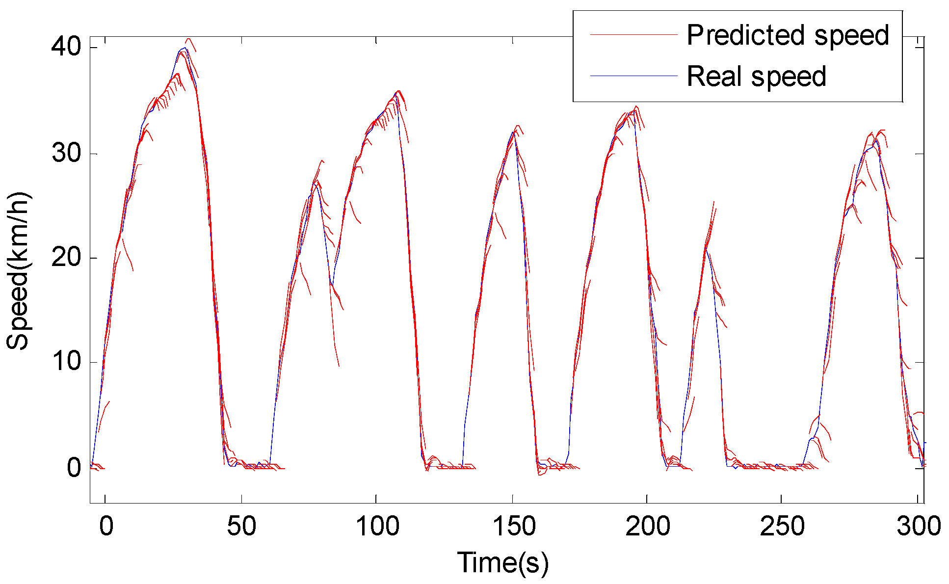
The short-term future vehicle speed in each receding horizon can be obtained through the proposed speed prediction method in Section 3. Then the predicted vehicle speed is used to calculate the vehicle required torque at each moment within the receding horizon. The proposed MLD-MPC control strategy aims to distribute the vehicle required torque between motor and engine reasonably at each moment within the prediction horizon to achieve optimal fuel economic. Thus MLD model is established to tackle this optimization problem with the objective function of equivalent fuel consumption, the control variable of motor torque u(k) and the state variable of SOC x(k). The optimal control variable sequence are obtained by minimizing the total equivalent fuel consumption in the receding horizon through MLD model and only the first control variable need to be applied in the controlled PHEV model at the present moment. The MLD-MPC receding horizon control procedure is described as follows:

(1)

at time k, predict the short-term future speed profile for the current control horizon (k–k + N, where N is the receding horizon) and calculate the corresponding required torque through Equations (1) and (2);

(2)

the MLD model calculates the optimal control policy (u(k)–u(k + N)) for the current prediction horizon (k–k + N);

(3)

apply the first time-step of the optimal control policy u(k) in the controlled PHEV model;

(4)

update the state variable and system constraints, repeat the computation procedure 1–3 at the next time instant (time k + 1).

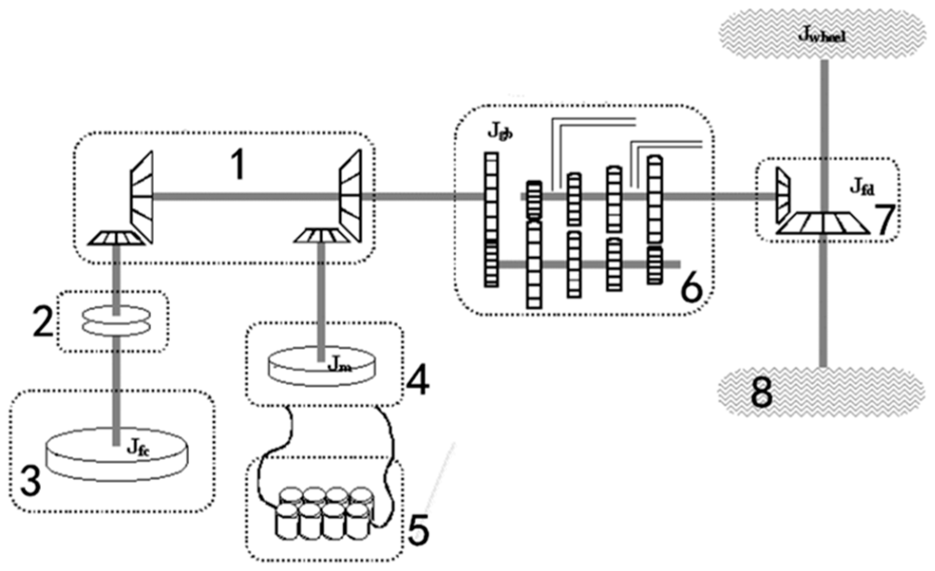
MLD model is suitable for solving problems combining binary variables and continuous variables. In [28], a constrained optimal problem is formulated and solved based on MPC using the simplified MLD model for DC-DC boost converter. Similarly, in our PHEV energy management control strategy, based on the simplified powertrain model in Section 2, the state transition equation and evaluation equation of MLD model can be described in Equation (10):

$$\{\begin{array}{l}x(k+1)=x(k)+B_1\mathsf{\delta }(k)+{\mathbf{B}}_2\mathbf{z}(k)\\ y(k)=D_1\mathsf{\delta }(k)+{\mathrm{D}}_2\mathbf{z}(k)\end{array}$$

(10)

where,

• $\begin{array}{cc}\hfill B_1& =[b_0(k)0b_0(k)b_0(k)b_0(k)0]\hfill \end{array}$
• $\begin{array}{cc}\hfill B_2& =[b_1(k)0b_1(k)b_1(k)b_1(k)0]\hfill \end{array}$
• $\begin{array}{cc}\hfill D_1& =[-\mathsf{\lambda }{U}_0{b}_0(k)Q_{\max }/R,a_0(k)+a_1(k)T_{in}(k),-\mathsf{\lambda }{U}_0{b}_0(k)Q_{\max }/R+a_0(k)+a_1(k)T_{in}(k),\hfill \\ & -\mathsf{\lambda }{U}_0{b}_0(k)Q_{\max }/R+a_0(k)+a_1(k)T_{in}(k),0,0]\hfill \end{array}$
• $\begin{array}{cc}\hfill D_2& =[-\mathsf{\lambda }{U}_1{b}_0(k)Q_{\max }/R,0,-\mathsf{\lambda }{U}_0{b}_1(k)Q_{\max }/R-i_t{a}_1(k),\hfill \\ & -\mathsf{\lambda }{U}_0{b}_1(k)Q_{\max }/R-i_t{a}_1(k)-\mathsf{\lambda }{U}_0{b}_1(k)Q_{\max }/R,0]\hfill \end{array}$

where $x(k)$ is the SOC of battery at time k, $y(k)$ is the equivalent rate of fuel consumption at time k, $\mathsf{\delta }(k)$ is the operation mode matrix at time k, which is a $6\times 1$ matrix whose entries are either 0 or 1 (logic variables), and only one of the six elements of the matrix is 1 and others are all 0. $\mathbf{z}(k)$ is the auxiliary variable, $\mathbf{z}(k)=\mathsf{\delta }(k)\cdot u(k)$, in which u(k) is the control variable which represents the torque of electric motor, and its inequality constraints are described in Equation (11). $i_t$ is the transmission ratio of the torque coupler which connects the engine to the motor. In the equation, the variables are obtained based on the linearized engine and battery model in Section 2. 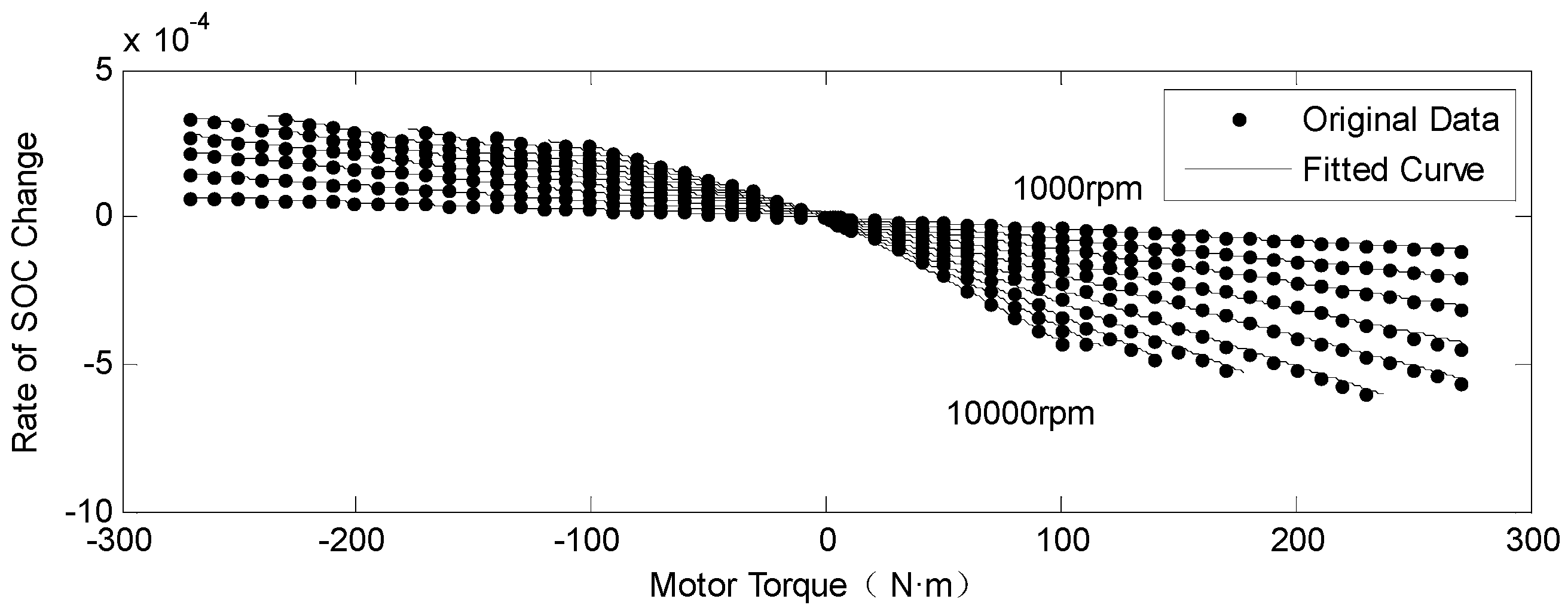B₁, B₂ is used to calculate the SOC change corresponding to the specific motor torque, b₀(k) and b₁(k) are the fitting coefficients for the specific motor speed at time k, and they are obtained from Equation (8). 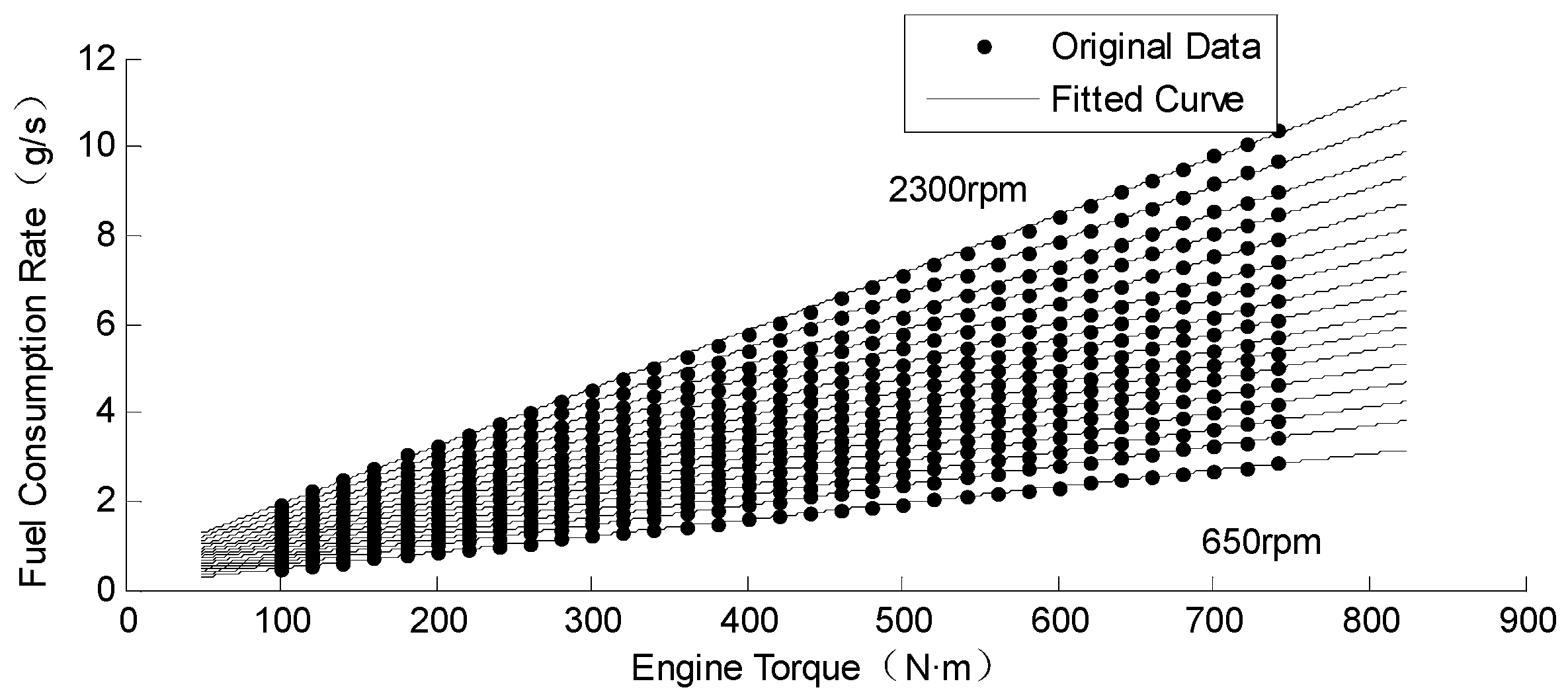Similarly, D₁ and D₂ is used to calculate the sum of engine fuel consumption and motor equivalent fuel consumption, a₀(k) and a₁(k) are from Equation (4):

$$\begin{array}{l}-T_M\mathsf{\delta }(k)+\mathbf{z}(k)\le 0\\ -T_M\mathsf{\delta }(k)-\mathbf{z}(k)\le 0\\ T_M\mathsf{\delta }(k)+\mathbf{z}(k)-u(k)\le T_M\\ T_M\mathsf{\delta }(k)-\mathbf{z}(k)+u(k)\le T_M\end{array}$$

(11)

The inequality constraint of the six operation modes for PHEV presented in

Table 4. Constraints during various operation mode for PHEV.

Electric Power Mode	Drive Charging Mode
$\{\begin{array}{c}{M}_{in}{\mathsf{\delta }}_1\le M_{in}+T_{in}-\mathsf{\epsilon }\hfill \\ M_{in}{\mathsf{\delta }}_1\le M_{in}-T_{in}+i_t{T}_{m\_\max }\hfill \\ -T_{in}{\mathsf{\delta }}_1+i_t{z}_1\le 0\hfill \\ T_{in}{\mathsf{\delta }}_1-i_t{z}_1\le 0\hfill \end{array}$	$\{\begin{array}{c}{M}_{in}{\mathsf{\delta }}_4\le -i_{t}u+M_{in}+T_{in}-\mathsf{\epsilon }\hfill \\ M_{in}{\mathsf{\delta }}_4\le i_{t}u+M_{in}-T_{in}+T_{e\_\max }\hfill \\ M_m{\mathsf{\delta }}_4\le u+M_m+T_{m\_\max }\hfill \\ M_m{\mathsf{\delta }}_4\le -u+M_m-\mathsf{\epsilon }\hfill \end{array}$
Fuel Consumption Mode	Regenerate Braking Mode
$\{\begin{array}{c}{M}_{in}{\mathsf{\delta }}_2\le M_{in}+T_{in}-\mathsf{\epsilon }\hfill \\ M_{in}{\mathsf{\delta }}_2\le M_{in}-T_{in}+T_{e\_\max }\hfill \\ z_2\le 0\hfill \\ -z_2\le 0\hfill \end{array}$	$\{\begin{array}{c}{M}_{in}{\mathsf{\delta }}_5\le M_{in}-T_{in}-\mathsf{\epsilon }\hfill \\ -T_{acc\_\max }{\mathsf{\delta }}_5+z_5\le 0\hfill \\ T_{acc\_\max }{\mathsf{\delta }}_5-z_5\le 0\hfill \end{array}$
Mixed Driven Mode	Stopping Mode
$\{\begin{array}{c}{M}_{in}{\mathsf{\delta }}_3\le -i_{t}u+M_{in}+T_{in}-\mathsf{\epsilon }\hfill \\ M_{in}{\mathsf{\delta }}_3\le i_{t}u+M_{in}-T_{in}+T_{e\_\max }\hfill \\ M_m{\mathsf{\delta }}_3\le u+M_m-\mathsf{\epsilon }\hfill \\ M_m{\mathsf{\delta }}_3\le -u+M_m+T_{m\_\max }\hfill \end{array}$	$\{\begin{array}{c}{T}_{in}{\mathsf{\delta }}_6\le 0\hfill \\ -T_{in}{\mathsf{\delta }}_6\le 0\hfill \\ z_6\le 0\hfill \\ -z_6\le 0\hfill \end{array}$

includes electric power mode, fuel consumption mode, mixed driven mode, drive charging mode, regenerate braking mode and stopping mode. The constraint describes the relationship of motor torque u and the vehicle required torque $T_{in}$ in each operation mode. In Table 4, $M_m$ and $M_{in}$ are the maximum motor torque and vehicle required torque respectively; $T_{e\_\max }$ and $T_{m\_\max }$ are the maximum engine torque and motor torque respectively; $T_{dec\_\max }$ is the maximum regenerative braking torque; $T_{dec\_\max }=\max (T_{in}/i_t,-T_{m\_\max })$; $\mathsf{\epsilon }$ is the machine accuracy, $\mathsf{\epsilon }$ = 0.0001; $T_{in}$ is the required torque, which can be can be calculated from Equations (1) and (2); ${\mathsf{\delta }}_i$ is the logic variable representing the operation mode of the vehicle (if ${\mathsf{\delta }}_i=1$, it means that the vehicle is running under the operation mode i); Consider the inequality constraints above into time sequence k and transfer them into the unified matrix inequality as follows, where E₁, E₂, E₃ and E₄ are all the coefficients in the form of Matrix converted from Table 4.

Applying receding horizon optimization based predictive control theory to the MLD model, and the optimal model is set-up as given in Equations (13) and (14), where the optimization metric is the sum of equivalent fuel consumption in the receding horizon at time k, the state transition and evaluation equality constraint are from Equation (10), the inequality constraints are taken from Equation (12):

$$E_1\mathsf{\delta }(k)+{\mathbf{E}}_2\mathbf{z}(k)\le E_{3}u(k)+E_4$$

(12)

$$\underset{\left\{u_k^k，u_k^{k+1}，u_k^{k+2}\mathrm{...}{u}_k^{k+N}\right\}}{\min }J={\displaystyle \sum _{i=0}^{N}y(k+i)}$$

(13)

s.t.

$$\{\begin{array}{l}{x}_{\min }(k)\le x(k)\le x_{\max }(k)\\ x(k+1)=x(k)+{\mathbf{B}}_1\mathsf{\delta }(k)+{\mathbf{B}}_2\mathbf{z}(k)\\ y(k)={\mathrm{D}}_1\mathsf{\delta }(k)+{\mathrm{D}}_2\mathbf{z}(k)\\ {\mathbf{E}}_1\mathsf{\delta }(k)+{\mathbf{E}}_2\mathbf{z}(k)\le {\mathbf{E}}_{3}u(k)+{\mathbf{E}}_4\end{array}$$

(14)

within it, B₁, B₂, D₁, D₂ is the same as Equation (10), and E₁, E₂, E₃, E₄, is defined as follows:

$${\mathbf{E}}_1=\left[\begin{array}{cccccc}{M}_{in}& 0& 0& 0& 0& 0\\ M_{in}& 0& 0& 0& 0& 0\\ -T_{in}& 0& 0& 0& 0& 0\\ T_{in}& 0& 0& 0& 0& 0\\ 0& M_{in}& 0& 0& 0& 0\\ 0& M_{in}& 0& 0& 0& 0\\ 0& 0& 0& 0& 0& 0\\ 0& 0& 0& 0& 0& 0\\ 0& 0& M_{in}& 0& 0& 0\\ 0& 0& M_{in}& 0& 0& 0\\ 0& 0& M_m& 0& 0& 0\\ 0& 0& M_m& 0& 0& 0\\ 0& 0& 0& M_{in}& 0& 0\\ 0& 0& 0& M_{in}& 0& 0\\ 0& 0& 0& M_m& 0& 0\\ 0& 0& 0& M_m& 0& 0\\ 0& 0& 0& 0& M_{in}& 0\\ 0& 0& 0& 0& -T_{acc\_\max }& 0\\ 0& 0& 0& 0& T_{acc\_\max }& 0\\ 0& 0& 0& 0& 0& T_{in}\\ 0& 0& 0& 0& 0& -T_{in}\\ 0& 0& 0& 0& 0& 0\\ 0& 0& 0& 0& 0& 0\\ -M_m& -M_m& -M_m& -M_m& -M_m& -M_m\\ -M_m& -M_m& -M_m& -M_m& -M_m& -M_m\\ M_m& M_m& M_m& M_m& M_m& M_m\\ M_m& M_m& M_m& M_m& M_m& M_m\end{array}\right]$$

In the equation, N is the prediction horizon, k is the specific second in the prediction horizon, $x_{\min }\left(k\right)$ and $x_{\max }\left(k\right)$ are the upper and lower limit of SOC accessible domains respectively at time k. Considering the values of matrices B₁, B₂, D₁, D₂, E₁, E₂, E₃ and E₄ at every sampling time k and according to the objective function of minimal equivalent fuel consumption, Equations (13) and (14) can be converted into a MILP problem.

4.2. Solution of Mixed Integer Linear Programming

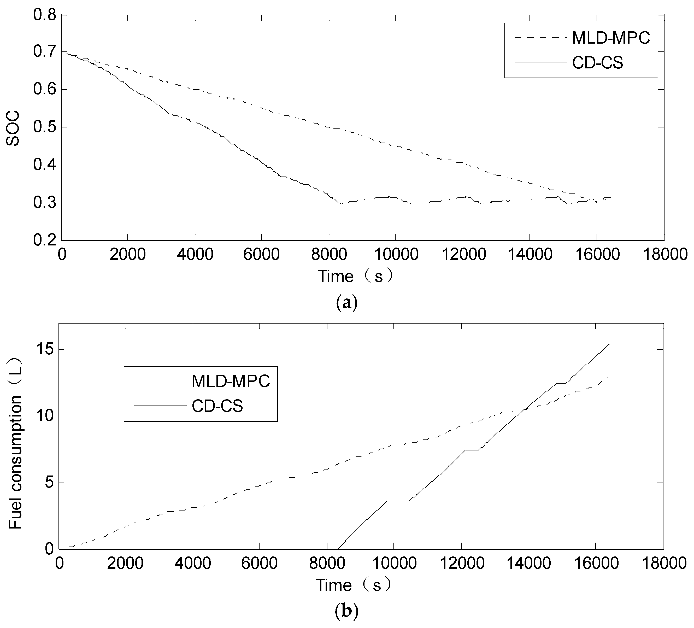
The MILP problem can be modeled using YALMIP toolbox in the Matlab platform and solved using the Gurobi optimizer. The optimal control variable sequence (u(k)–u(k + N)) in the prediction horizon (k–k + N) can be calculated at time k, and the first value of the optimal control variable sequence u(k) is applied to the controlled object. Then utilizing the receding horizon optimization method, the former solving steps are repeated to get a new control value at time k + 1 to realize the PHEV MPC. In the process of updating the model state variable, SOC, the original nonlinear model as shown in Equation (6) is used instead of the simplified linear equality constraint model in MILP to obtain a better estimate of the true SOC value at the end of the control time domain. The obtained value is considered as the initial state value to the next receding horizon optimization, so as to realize the feedback correction in predictive control.

Heuristic rules for some special driving conditions are set to reduce the range of feasible solution of MILP and improve the real-time performance of the control strategy. The introduced heuristic rules are presented in

Table 5. Heuristic rules.

Driving Condition	Operation Mode	Motor Torque Decision
$T_{in}=0$	${\mathsf{\delta }}_6=1$	$u=0$
$T_{in}<0$	${\mathsf{\delta }}_5=1$	$u=T_{in}/i_t$
$SOC<SO{C}_{\min }$	${\mathsf{\delta }}_4=1$	$u=(T_{in}-T_{e\max })/i_t$
$T_{in}>T_{e\_\max }$	${\mathsf{\delta }}_3=1$	$u>0,0<T_{in}-i_{t}u<T_{e\_\max }$
Else	${\mathsf{\delta }}_1=1$	$u=T_{in}/i_t$
	${\mathsf{\delta }}_2=1$	$u=0$
	${\mathsf{\delta }}_3=1$	$u>0,0<T_{in}-i_{t}u<T_{e\_\max }$
	${\mathsf{\delta }}_4=1$	$u<0,0<T_{in}-i_{t}u<T_{e\_\max }$

. While the condition in the first column is satisfied, the corresponding operation mode $\mathsf{\delta }(k)$ and motor torque can be decided respectively. Total required torque $T_{in}$ can be used as a measure to judge whether the car is braking or stopping. Based on the value of total required torque, whether it is less than or equal to zero, the vehicle can choose regenerate braking mode or stop mode directly, and the corresponding control variable value can be determined directly. When the vehicle is in urgent acceleration or at high speed, and the total inquired torque is larger than the maximum engine torque at that speed, the vehicle can choose mixed driven mode directly. Otherwise, the control strategy can switch among four modes, i.e., electric power mode, fuel consumption mode, mixed driven mode, drive charging mode. The control variable value in electric power mode and fuel consumption mode can be directly obtained. The control variable in the mixed driven mode and drive charging mode can be selected through the optimization of the objective function. These heuristic rules can significantly reduce the search space of MILP and thus improve the efficiency of the algorithm.

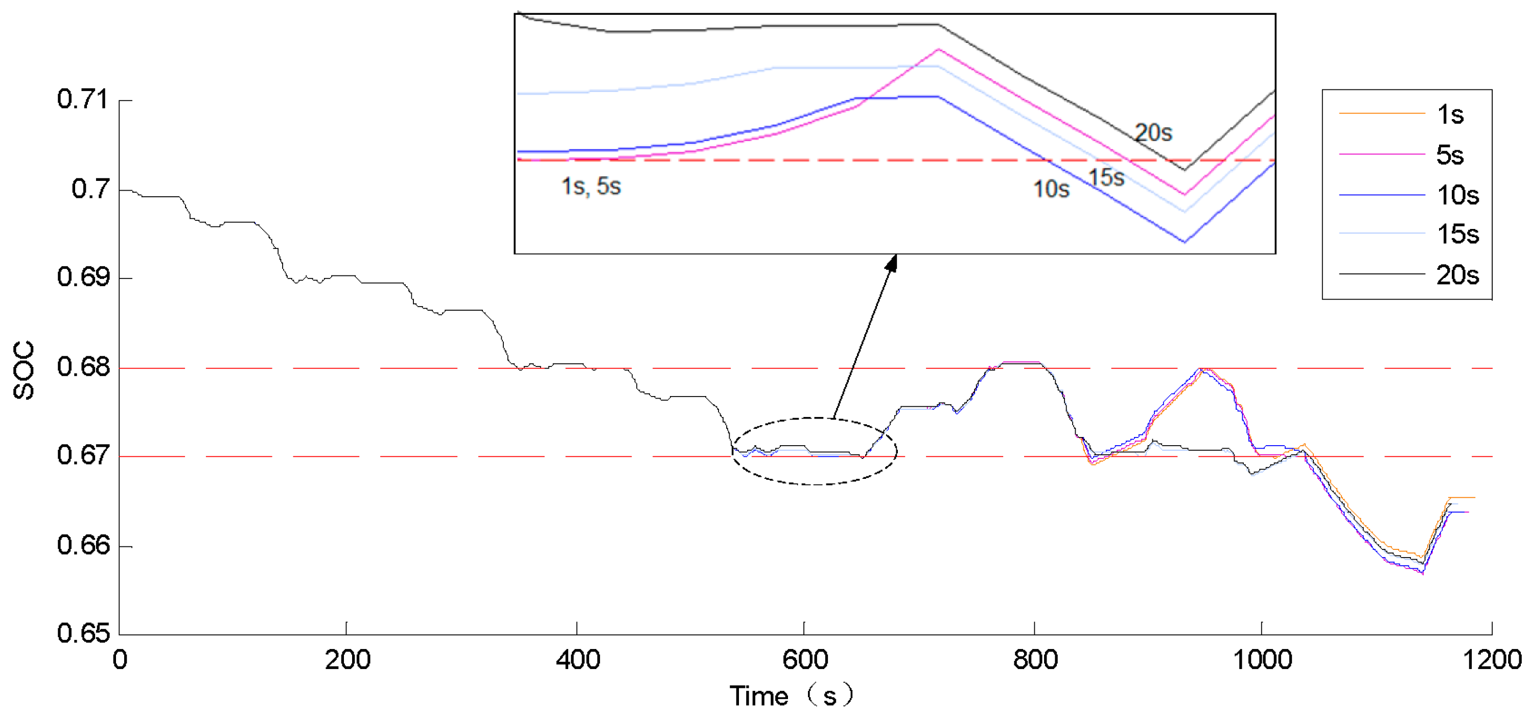
When SOC approaches to the lower limit, once the required torque is larger than the maximum torque of the engine and the objective function in MLD-MPC is not modified, the motor needs to output the power which would make the SOC of the battery to exceed the lower limit. This violates the constraints defined in MILP problem and cannot find a feasible solution. Thus, when SOC is around the lower limit, the heuristic rule is applied to solve the control problem. First, estimate the highest SOC at each step in the prediction horizon under the assumption that the engine outputs its maximum torque. If the estimated highest SOC is higher than the lower limit of SOC, the current SOC constraints are imposed in MILP, otherwise the corresponding SOC constraints will be removed. When the current SOC is lower than the lower limit of SOC, the algorithm will stop solving the MILP problem and change to the heuristic solver mode. In this mode, the maximum charging torque (or the minimum discharging torque) of the motor is calculated directly while the engine is set to output its maximum torque. After the SOC rises to a certain value higher than the lower limit of SOC, the MILP solver will be restarted.

5. Simulation Experiments and Analysis

5.1. Simulation Experiments

Parameters of the PHEV are given in

Table 6. Parameters of the PHEV.

Parameter	Value	Unit
Maximum mass	13,485	kg
Air resistance coefficient	0.79	-
Frontal area	7.24	m2
Wheel rolling radius	0.5	m
Rolling resistance coefficient	0.0094	-
Wheel base	6.85	m
Final ratio	1	-
Rotational inertia of wheels in total	20.5215	$\mathrm{kg}\cdot {\mathrm{m}}^2$
Rotational inertia of engine and motor	2.2511	$\mathrm{kg}\cdot {\mathrm{m}}^2$

. The diesel engine displacement is 7.3 L with a rated power of 177 kW, and maximum engine speed is 2300 r/min.

The type of motor is AC induction motor, with rated power of 124 kW, and maximum motor speed of 10,000 r/min. The type of battery used is a lithium battery with a rated capacity of 90 $\mathrm{A}\cdot \mathrm{h}$. M_m is 272 N·m, and M_in is 1170 N·m. Fitting coefficients of engine and motor are listed in the Appendix A. ADVISOR (Advanced Vehicle Simulator, 2002, National Renewable Energy Laboratory, Golden, CO, USA) is used to simulate the UKBUS driving cycle as shown in Figure 11, with an initial SOC value of 0.7 ($0.3\le SOC\le 0.8$), prediction horizon N of 15 s and sampling period of 1 s (the effect of predict time domain is discussed in Section 5.2). The simulation results are presented in Figure 12. Figure 12a is the comparison of the SOC curves between the MLD-MPC control strategy proposed in this paper and Charge Depleting-Charge Sustaining (CD-CS) control strategy. As can be observed, the CD-CS strategy consumes the battery energy within 8000 s, and then sustains SOC around 0.3 for the remainder of the trip. In the MLD-MPC control strategy, the battery energy is completely consumed by the end of the trip. Compared to CD-CS control strategy, the proposed MLD-MPC strategy can make more reasonable use of battery energy. Figure 12b is the comparison of the fuel consumption between the MLD-MPC control strategy presented in this paper and CD-CS control strategy. As seen in the picture, the CD-CS control strategy makes full use of battery energy and does not consume fuel within the first 8000 s, then the fuel consumption grow rapidly during the Charge-Sustaining mode, while the MLD-MPC control strategy maintains a relatively slow fuel consumption rate. Up to the end of the whole driving cycle, the fuel consumption is 12.93 L, and the end value of SOC is 0.3043 for the MLD-MPC control strategy, while the fuel consumption is 15.39 L, and the end value of SOC is 0.3125 for the CD-CS control strategy. It can be concluded from this results that under the same driving cycle conditions, the MLD-MPC control strategy reduces the fuel consumption of a PHEV. Figure 13 shows the comparison of engine operation points of these two control strategies. As can be observed, the engine operation points of the CD-CS control strategy spread out on a much larger area, and a lot of operation points in the low efficiency area. While the engine operation points of MLD-MPC control strategy is relatively centralized and most of them are in the high efficiency area which will improve fuel economic.

Besides the simulation of UKBUS driving cycle, driving cycles of Orange County Bus Cycle (OCC) and New European Drive Cycle (NEDC) are simulated as well. The results can be seen in

Table 7. Fuel consumption under two control strategies. NEDC: New European Drive Cycle; OCC: Orange County Bus Cycle.

Driving Cycle	Control Strategy	Final SOC	Fuel Consumption (L)	Fuel Saved
5 × UKBUS	MLD-MPC	0.3043	12.93	15.98%
	CD-CS	0.3125	15.39
8 × NEDC	MLD-MPC	0.2939	12.46	14.36%
	CD-CS	0.2743	14.55
8 × OCC	MLD-MPC	0.2959	15.95	7.27%
	CD-CS	0.3023	17.20

, which shows that the fuel economy of PHEV under these driving cycles is improved to a noticeable extent.

5.2. Influence of Prediction Horizon for Mixed Logic Dynamical-Model Predictive Control (MLD-MPC) Strategy

Two key steps are included in the MLD-MPC control strategy proposed in this paper, which are NAR neural network based vehicle speed prediction and minimal fuel consumption objective function-based MLD model prediction control. With an increase in prediction horizon, the accuracy of prediction results will decrease compared to the actual speed and thus affect the accuracy of the MPC solution and increase the fuel consumption. The MPC uses the online receding horizon optimization within the limited horizon, and when the optimal horizon increases, the optimization performance index also increases which leads to better results. Therefore, it is important to find out the proper prediction horizon for the optimal fuel consumption simulation.

Here, NEDC is used to study the effect of prediction horizon length on target equivalent fuel consumption. And the same NAR neural network training method as for UKBUS is utilized for NEDC. With a total of 1190 samples of vehicle speed-intention data, the first 900 samples are chosen as training samples, and the remaining 290 samples which didn’t participate in the training are used to test the network’s predictive ability. When the value of SOC does not drop to the lower limit value, the constraints of state variable SOC are not activated. The optimal control variable can be solved independently, and the function of prediction horizon cannot be reflected, as the state association of each second is not restricted by constraints within the prediction horizon. The function of prediction horizon is realized only when the value of SOC is going to cross the lower limit. Therefore, initial SOC value of 0.7 is selected and the lower limit of SOC is set to 0.67 to simulate the condition that SOC is going to reach the lower limit. In this phase, heuristic solver mode will be activated to recharge the batteries up to 0.68 when SOC falls below 0.67 and then MILP solver mode will be selected.

Figure 14 shows the battery SOC curve under different prediction horizons, and the corresponding time to reach the lower limit of SOC value is shown in

Table 8. SOC bottoming time under different prediction horizons.

	Bottoming Time	First Bottoming	Second Bottoming
Prediction Horizon
1 s		643 s	847 s
5 s		643 s	849 s
10 s		650 s	851 s
15 s		650 s	976 s
20 s		651 s	976 s
25 s		651 s	976 s
30 s		675 s	1040 s

. It can be seen that the time to reach the lower limit of SOC is extended as the prediction horizon increases. That is to say, in the process of optimization with MILP, it can predict in advance that SOC is about to reach the lower limit so the strategy can choose to save electricity in advance and improve the fuel efficiency. Figure 15 shows the equivalent fuel consumption per hundred kilometers corresponding to the different prediction horizons.

The change of RMSE of the predicted speed with different prediction horizons is shown in Figure 16. Compared to Figure 15, with an increase in prediction horizon, the equivalent fuel deceases continuously until the prediction horizon reaches 15 s, while the equivalent fuel consumption deceased only a little when the prediction horizon is increased from 15 s to 30 s. However, RMSE of the predicted speed is significant increased when the prediction horizon is increased from 15 s to 30 s. Therefore, a prediction horizon of 15 s is chosen in this paper.

6. Conclusions

A MPC strategy for PHEV based on a MLD model and vehicle speed prediction was proposed in this paper. Firstly, to convert the PHEV control problem into a linear programming problem, the energy consumption model of engine and motor were both linearized. After that, focusing on a city bus which usually has determined routes and known velocity profiles, a vehicle speed prediction method using a NAR neural network based on the combination of driving intention and historical speed data was proposed, in which the driving intention is recognized by using fuzzy inference to analyze the driver’s pedal operation. Then, a vehicle MLD model is established with constraints in six possible driving modes and an objective function of minimum equivalent fuel consumption. With the predicted vehicle speed, a MPC method was utilized and the energy management problem was converted to a MILP problem, and the optimal motor torque and the corresponding driving mode sequence within the speed prediction horizon can be solved. The simulation was carried out under three driving cycles, and the effect of prediction horizon on the result of the simulation is analyzed, the simulation results verified the feasibility and effectiveness of the vehicle speed prediction based MLD-MPC strategy.