
A Frequency Control Approach for Hybrid Power System Using Multi-Objective Optimization

 ,
,  ,
,
Abstract
:1. Introduction
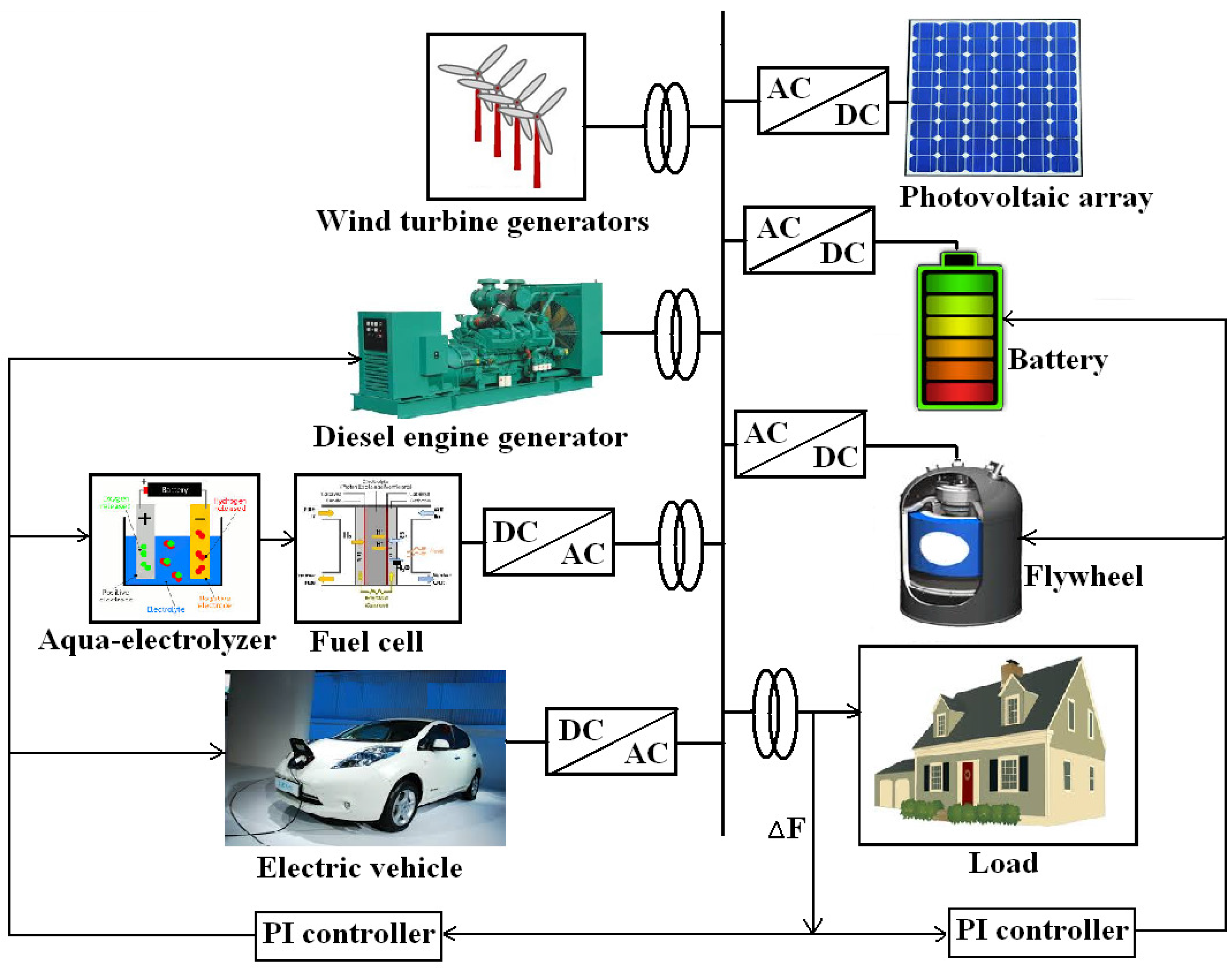
2. Hybrid Power System Configuration
2.1. Wind Turbine Generator Model
2.2. Photovoltaic Model
2.3. Power and Frequency Deviations
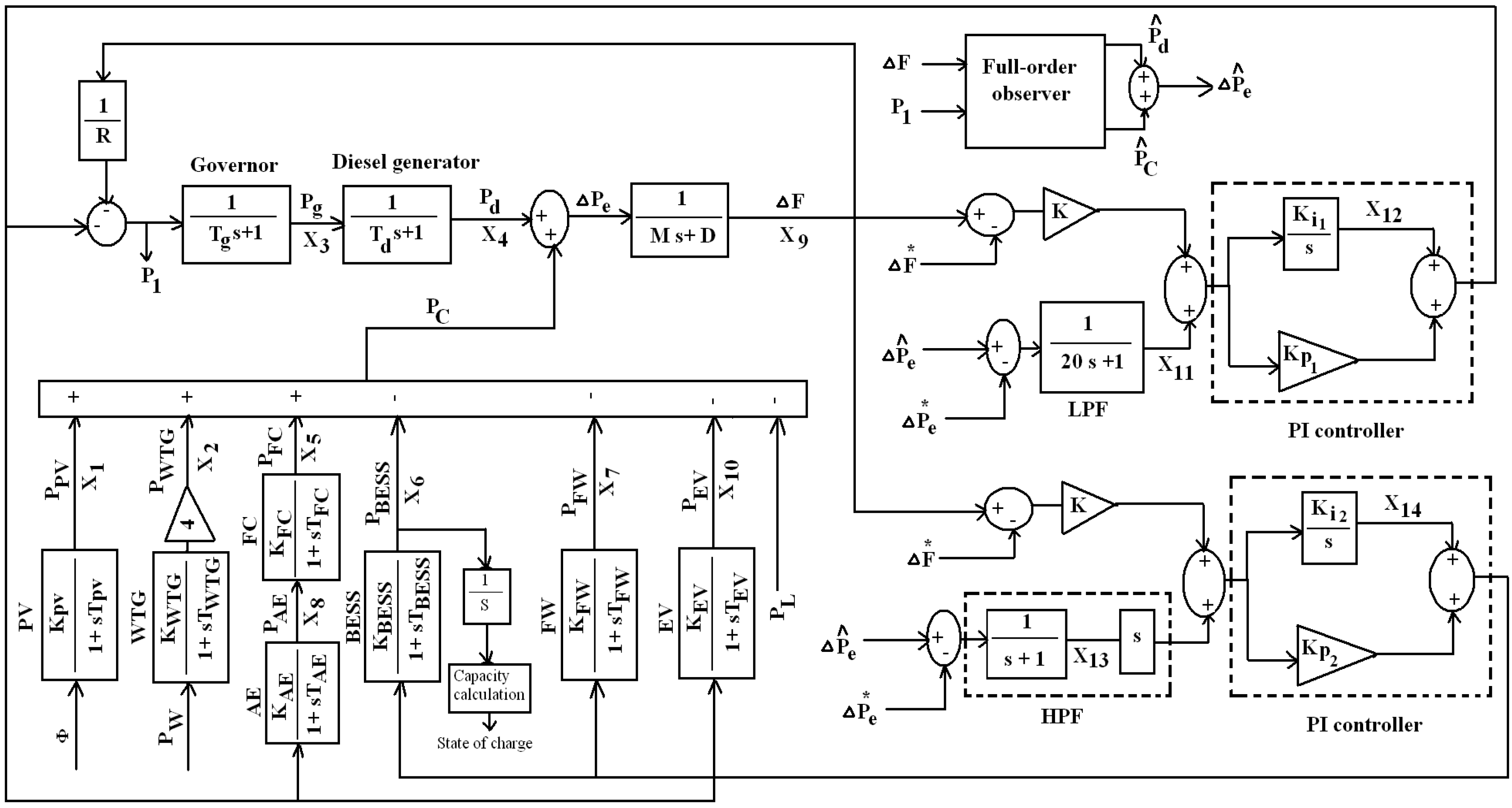
3. Controllers’ Design Approach
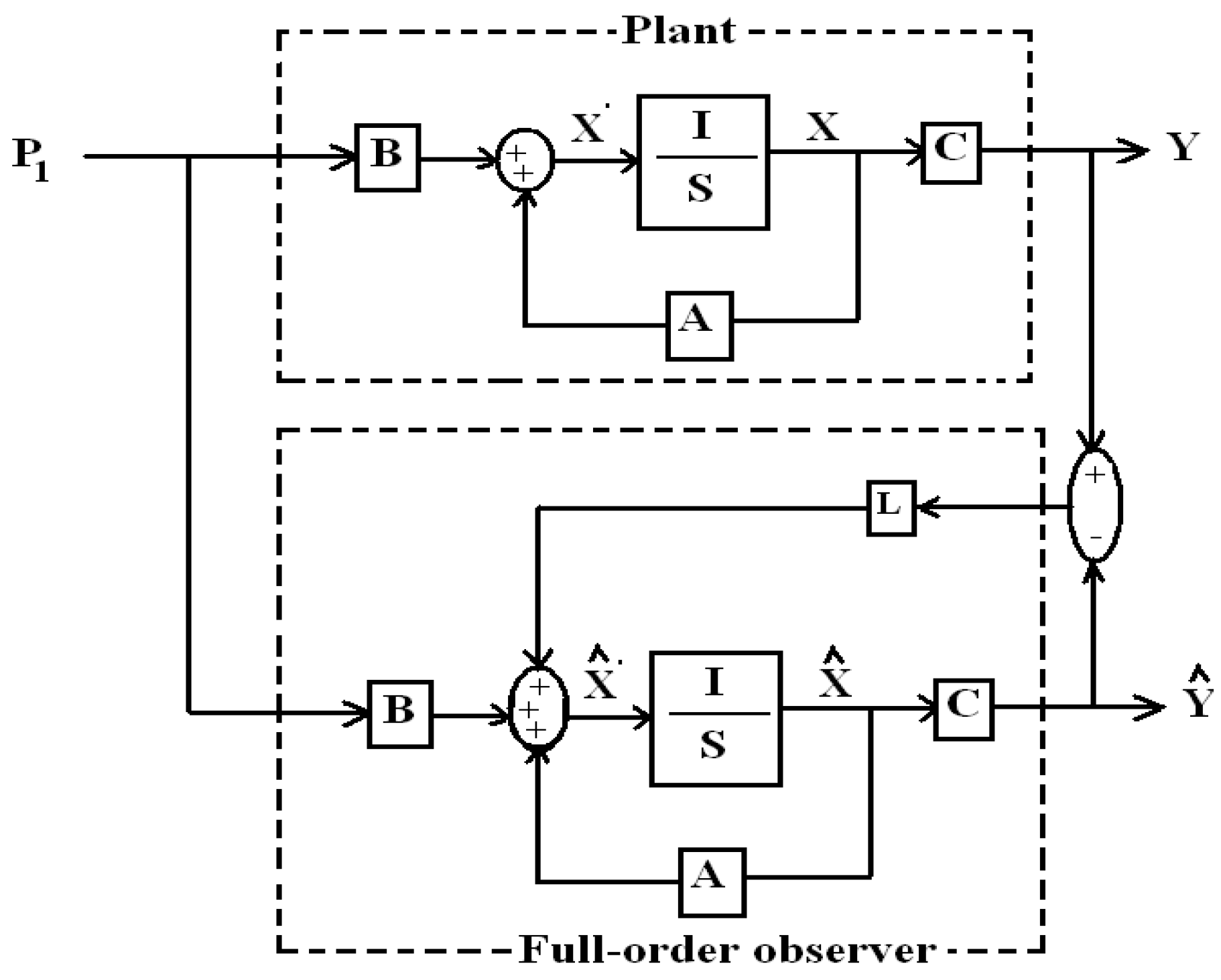
3.1. Full-Order Observer Implementation
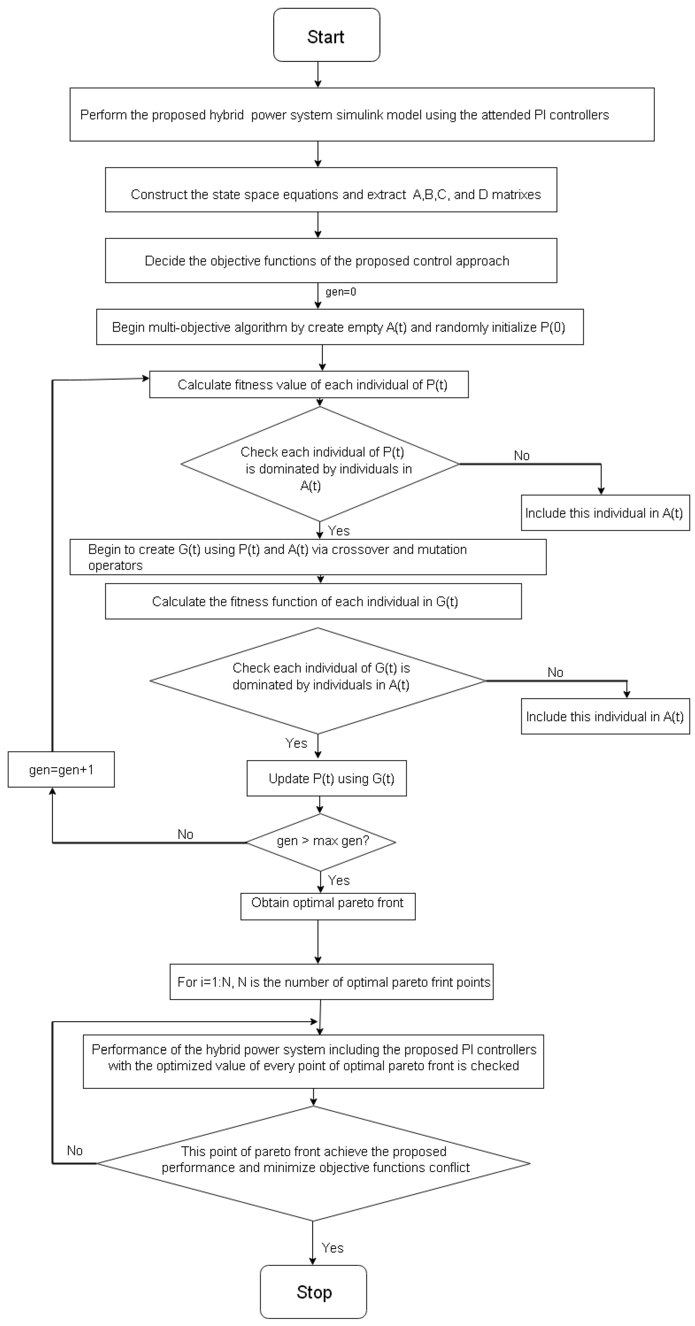
3.2. Epsilon Multi-Objective Genetic Algorithm (-MOGA) Theory
- Step 1.
- Begin and create empty A(t).
- Step 2.
- P(0) is initialized with individuals that have been randomly selected from .
- Step 3.
- Calculate the function value of each individual in P(t).
- Step 4.
- Check individuals in P(t) that might be included in A(t), as follows:
- (1)
- Non-dominated individuals in P(t) are detected, .
- (2)
- Pareto front limits and are calculated from (x), ∀ x .
- (3)
- Individuals in are analyzed, and those that are not -dominated by individuals in A(t) are included in A(t).
- Step 5.
- Create G(t) as follows:
- (1)
- Two individuals are randomly selected, from P(t) and from A(t).
- (2)
- A random number u [0…1] is generated.
- (3)
- If u > (probability of crossing/mutation), and are crossed over by means of the extended linear recombination technique.
- (4)
- If u < , and are mutated using Gaussian distribution and then included in G(t).
- Step 6.
- Calculate the function value of each individual in G(t).
- Step 7.
- Checks, one by one, which individuals in G(t) must be included in A(t) on the basis of their location in the objective space.
- Step 8.
- Update P(t) with individuals from G(t). Every individual from G(t) replaces an individual that is randomly selected from the individuals in P(t) that are dominated by . However, will not be included in P(t) if there is no individual in P(t) dominated by .Finally, individuals from A(t) compose the smart characterization of the Pareto front, .
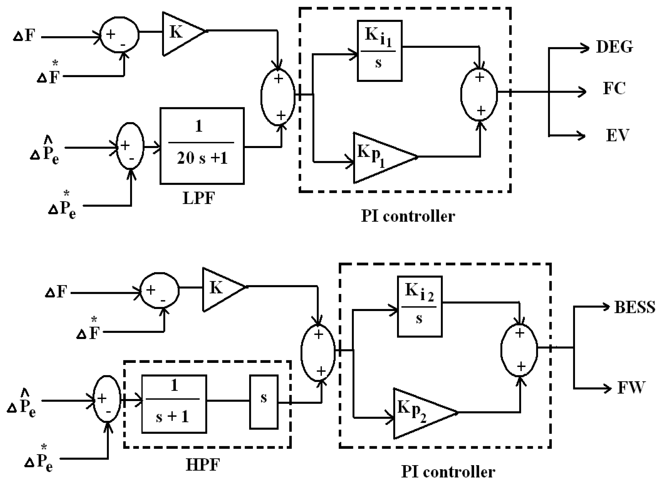
3.3. Epsilon Multi-Objective Genetic Algorithm (-MOGA)-Based PI Controllers’ Scheme
- = 10, = 25,000, = 0.25.
- Number of generations 12,000.
- = = 600.
4. Results
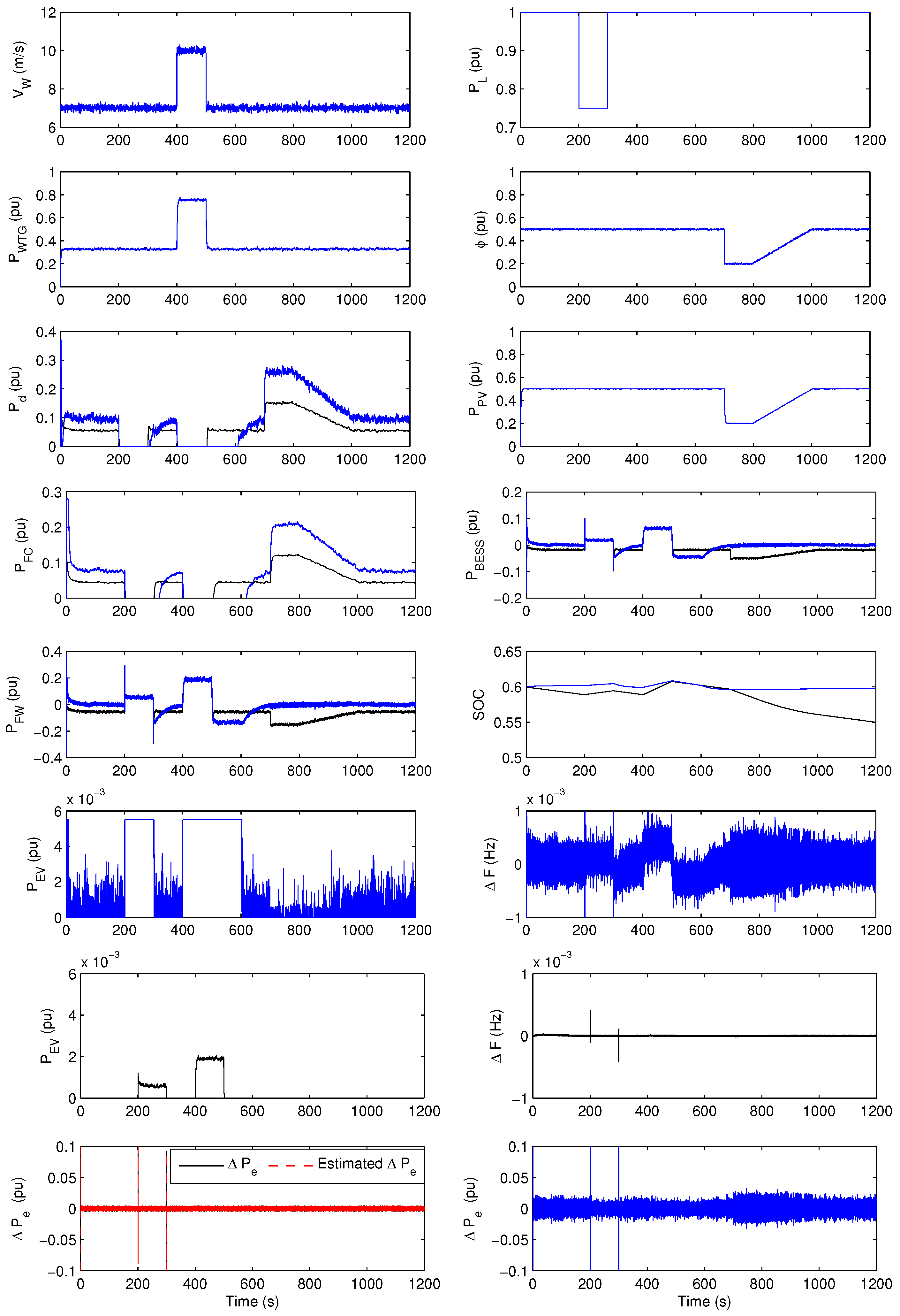
4.1. Case 1
- (1)
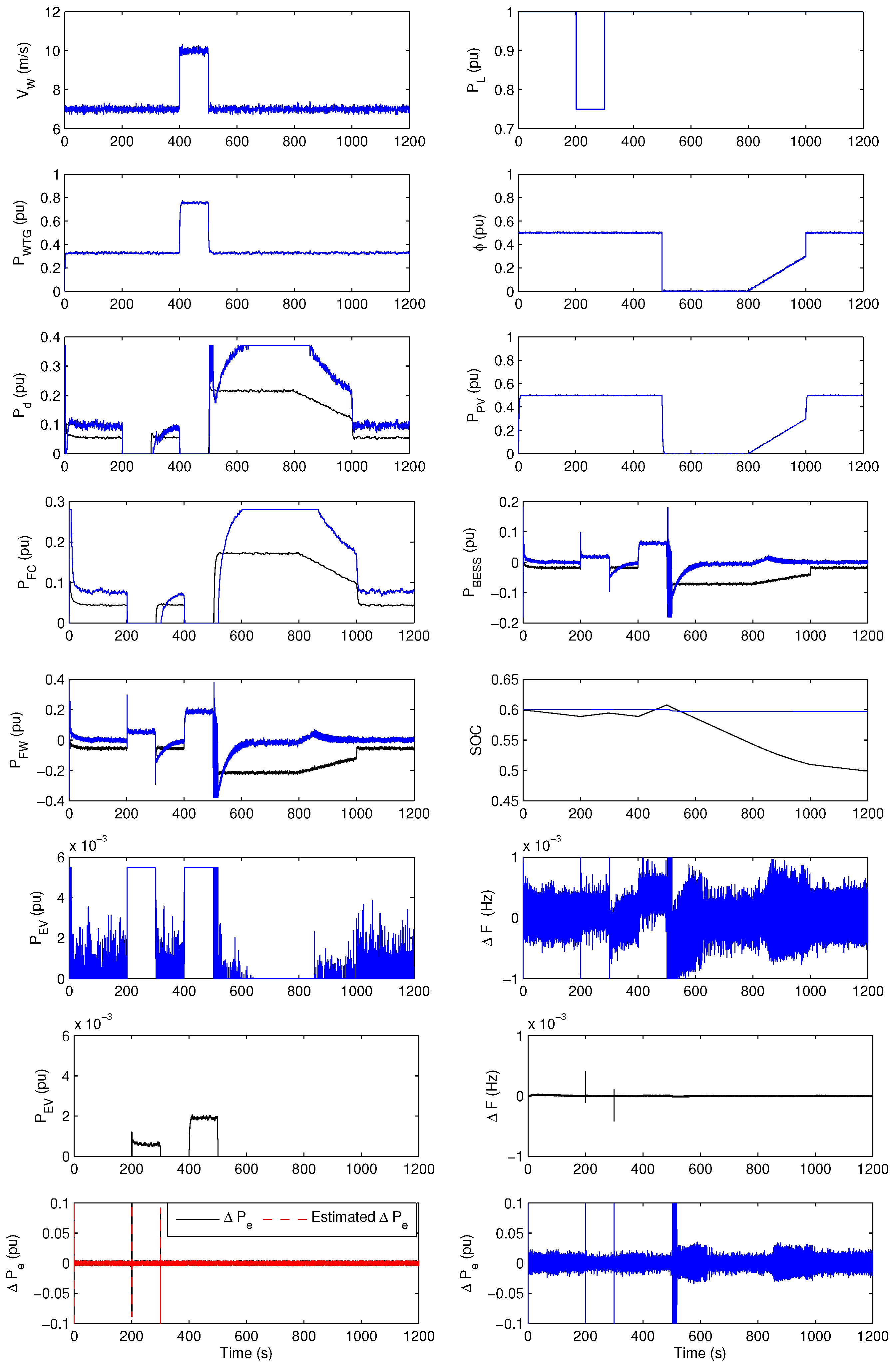
- Base case: Through 0 s < t < 200 s and 1000 s < t < 1200 s, the average solar radiation and wind speed are about 0.5 pu and 7.5 m/s, respectively. Depending on this, the average output powers of WTG units and the PV array are around 0.3 pu and 0.5 pu, respectively, with equal to 1 pu. Since with are not sufficient yet to meet demand alone, DEG and FC are connected automatically to the system at t = 0 s. Furthermore, BESS and FW begin to release power to the system trying to decrease the power shortage in this time. No surplus power can be used to charge EV in this interval, as shown in Figure 8. The proposed control scheme succeeded to suppress ΔF and also Δ fluctuations with a good estimate of the full-order observer as indicated in the figure, which illustrates Δ and estimated Δ. However, for the conventional approach, DEG and FC produce a larger amount of power compared to that of the proposed scheme with high fluctuations and overshoot, as shown in the figure. Therefore, BESS and FW decrease their released power in this interval, but still with high fluctuations. Furthermore, the charged power of EV fluctuates significantly. In addition, the conventional approach has clear oscillations for ΔF and Δ compared to the proposed one.
- (2)
- Sudden load drop: At 200 s < t < 300 s, and have the same values of the base case, but drops suddenly from 1 pu to 0.75 pu at t = 200 s. Consequently, and produce sufficient output power to meet in this case. Therefore, DEG and FC are automatically disconnected from the system at t = 200 s. EV starts to charge power from the system. Furthermore, BESS and FW begin to store excess power. In spite of the sudden load decrease, the proposed control approach still ensures adequate damping performance for ΔF and Δ deviations with a suitable estimate of the full-order observer. On the other hand, for the conventional control approach, EV charges to its capacity limit during this interval. Large fluctuations of ΔF and Δ still appear compared to the proposed approach.
- (3)
- Sudden load rise: During 300 s < t < 400 s, and still have the same values of the base case, but rises suddenly from 0.75 pu to 1 pu at t = 300 s. The hybrid power system returns to the same operating point of the base case. Therefore, all responses are the same as those in the interval 0 s < t < 200 s. The control technique still has the ability to damp ΔF and Δ fluctuations with robust performance of the observer, while the conventional control approach has a clear amount of fluctuations for ΔF and Δ.
- (4)
- Sudden wind speed rise: When 400 s < t < 500 s, the values of and are still 0.5 pu and 1 pu, respectively. However, suddenly increases from 7.5 m/s to 10 m/s at t = 400 s. Therefore, increases to around 0.8 pu, which is enough with to meet load demand in this period. Then, DEG and FC are totally disconnected from the system at t = 400 s. Furthermore, BESS, FW and EV start to store excess power from the system with a larger amount as compared to what happened in the interval 200 s < t < 300 s, as a result of more existing surplus power in the system due to the wind speed increase. Proposed controllers still mitigate ΔF and Δ fluctuations with effective performance of the full-order observer. For the conventional approach, oscillations of ΔF and Δ can be noticed clearly with a higher amplitude than that of the proposed control scheme.
- (5)
- Sudden wind speed drop: At 500 s < t < 700 s, suddenly decreases from 10 m/s to 7.5 m/s at t = 500 s. Therefore, returns to around 0.3 pu with the same values of and . The proposed power system comes back to the same operating condition of the base case. The simulation results are the same ones in the interval 0 s < t < 200 s. ΔF and Δ deviations are still in the acceptable limits, as shown in Figure 8, during this interval with the proper estimate of the full-order observer. However, for the conventional approach, the speed of response of DEG and FC was very slow to the sudden decrease of wind speed, while BESS and FW increase their released power to overcome this shortage. There are still large fluctuations of ΔF and Δ compared to the proposed approach.
- (6)
- Solar radiation sudden drop: During 700 s < t < 800 s, the values of and are still 7.5 m/s and 1 pu, respectively. However, drops to 0.2 pu suddenly. Therefore, also drops to 0.2 pu. Accordingly, DEG and FC are connected automatically to the system producing a larger amount of output power compared with previous intervals to compensate the drop in . Furthermore, BESS and FW begin to release power to the system. There is no surplus power to charge EV in this period. The proposed controllers damp all fluctuations of and with the perfect estimate of the full-order observer. On the other hand, for the conventional approach, DEG and FC produce output more power than that of the proposed approach. Therefore, BESS and FW decrease their released power during this interval. Large fluctuations appear for the charged power of EV,ΔF and Δ compared to the proposed approach.
- (7)
- Solar radiation linear increase: When 800 s < t < 1000 s, linearly increases in this interval from 0.2 pu to 0.5 pu, while and have constant values of 7.5 m/s and 1 pu, respectively. Hence, linearly increases also from 0.2 pu to 0.5 pu. Then, , and the released powers of BESS and FW linearly and slightly decrease to meet the power balance condition. There is no excess power to feed EV also in this period. The proposed control scheme still suppress and fluctuations, and the full-order observer has a good performance in this interval. For the conventional approach, no response for BESS and FW happened in this period, and large fluctuations still exist for ΔF, Δ and the charged power of EV.
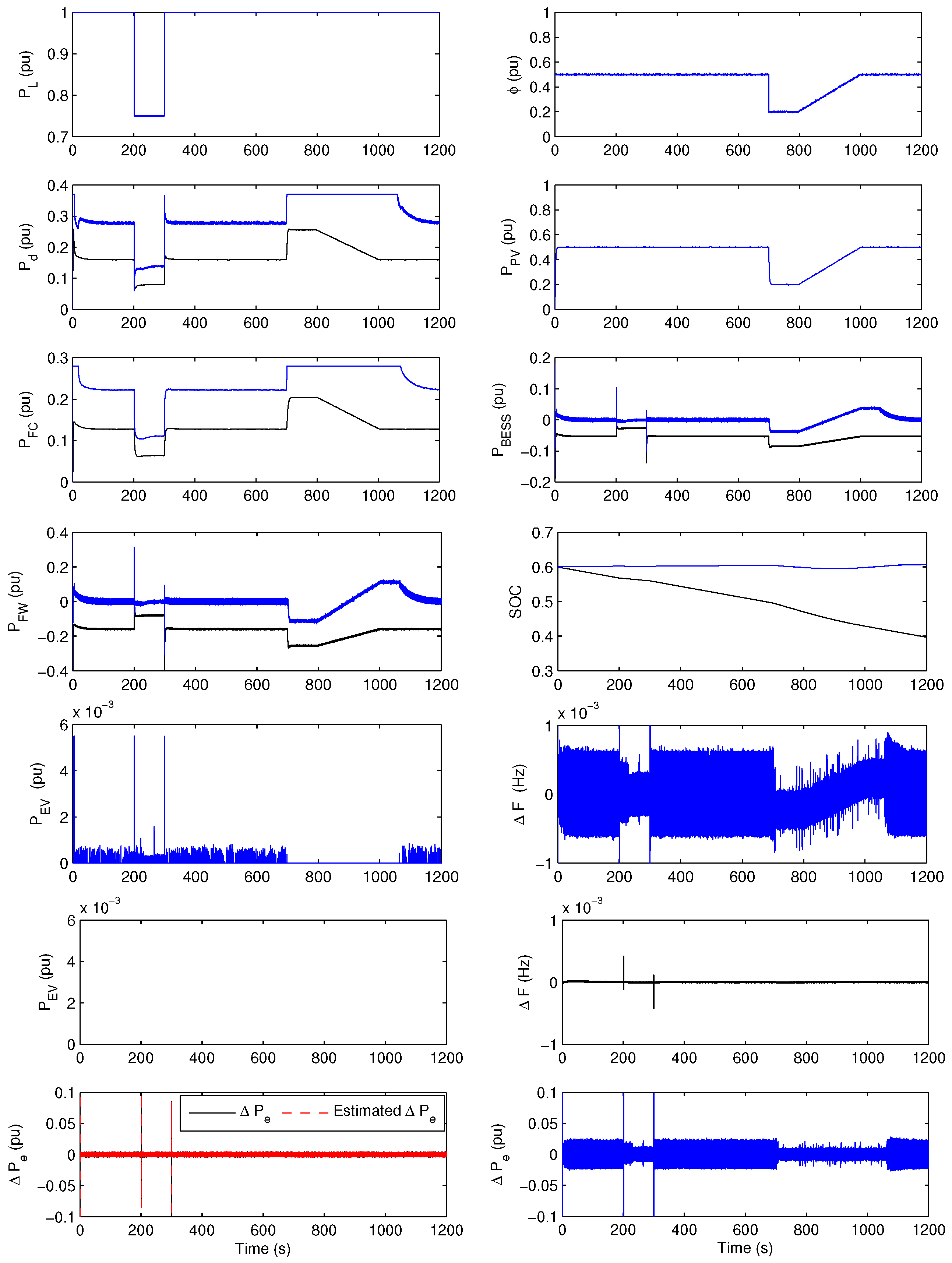
4.2. Case 2
- (1)
- Base case: Through 0 s < t < 200 s and 1000 s < t < 1200 s, the values of and are 0.5 pu and 1 pu, respectively. Therefore, the average output power of the PV array is about 0.5 pu. Due to the WTG units’ outage, is not enough to meet load demand. Therefore, DEG and FC are connected automatically to the system at t = 0 s, generating higher output power compared to the same interval in Case 1 to compensate the lack of generated power due to the outage of WTG units. Furthermore, BESS and FW start to release power to the system to face the shortage of generated power in this period. There is no excess power that can be utilized to charge EV, as shown in Figure 9. The proposed control approach damps all of the ΔF and Δ fluctuations with a good estimate of the full-order observer. On the other hand, for the conventional control approach, DEG and FC produce a larger amount of power with high fluctuations and overshoot compared to that of the proposed scheme, as shown in the figure. Therefore, BESS and FW decrease their released power in this interval. Furthermore, high fluctuations appear clearly for the charged power of EV, ΔF and Δ.
- (2)
- Sudden load drop: At 200 s < t < 300 s, the value of is still 0.5 pu. Therefore, has the same previous value of 0.5 pu, but decreases suddenly from 1 pu to 0.75 pu at t = 200 s. As a result, DEG and FC decrease their generated output power as the mismatch between generation and demand powers is reduced due to the sudden load drop. Furthermore, BESS and FW begin to decrease their released power to the system. No surplus power exists even in this period to charge EV. The proposed control technique still has the ability to mitigate ΔF and Δ deviations with a suitable estimate of the full-order observer, as shown in Figure 9. However, for the conventional control approach, large fluctuations still exist for ΔF, Δ and the charged power of EV compared to that of the proposed control scheme.
- (3)
- Sudden load rise: During 300 s < t < 700 s, increases suddenly from 0.75 pu to 1 pu at t = 300 s, and the value of is still 0.5 pu. Therefore, the power system comes back to the same operating point of the base case. All simulation responses are the same as those in the interval 0 s < t < 200 s. The control scheme succeeded to damp the ΔF and Δ fluctuations with the effective estimate of the observer, while the conventional control technique fails to damp the oscillations of charged power of EV, ΔF and Δ, as shown in Figure 9.
- (4)
- Solar radiation sudden drop: During 700 s < t < 800 s, is still 1 pu, but suddenly drops to 0.2 pu at t = 700 s. Therefore, also decreases to 0.2 pu. Consequently, DEG and FC increase their output power to compensate the sudden drop of and with values more than that in the same period of Case 1 due to the WTG units’ outage. Furthermore, BESS and FW release more power to meet the load demand in this interval. Still, there is no excess power to charge EV in this period. The proposed control approach still ensures keeping the ΔF and Δ deviations within the acceptable limits with the robust estimate of the full-order observer. For the conventional approach, fluctuations of ΔF and Δ still appear with a large value compared to that of the proposed technique.
- (5)
- Solar radiation linear increase: When 800 s < t < 1000 s, still has a constant value of 1 pu. However, linearly increases from 0.2 pu to 0.5 pu in this period. Therefore, also linearly rises from 0.2 pu to 0.5 pu. Accordingly, , and the discharged power of BESS and FW linearly decrease to achieve balance between generation and load demand in this interval. There is no surplus power to charge EV, as shown in Figure 9. The control mechanism is still able to suppress the ΔF and Δ fluctuations, and the full-order observer has adequate performance during this interval, as indicated in Figure 9. However, for the conventional approach, there is no response of DEG and FC due to the linear increase in solar radiation, and they still produce their maximum power. Figure 9 shows large fluctuations of ΔF and Δ compared to that of the proposed control scheme in this interval.
4.3. Case 3
- (1)
- Base case: When 0 s < t < 200 s and 1000 s < t < 1200 s, the values of , and are 7.5 m/s, 0.5 pu and 1 pu, respectively. Hence, the averages output powers of WTG units and the PV array are around 0.3 pu and 0.5 pu, respectively. DEG and FC are connected automatically to the system, supplying their output power due to the fact that and cannot meet the load demand alone in this interval. Furthermore, BESS and FW start to release their power to achieve the power balance condition. There is no excess power to charge EV in this period. The control approach is capable of damping ΔF and Δ fluctuations with a good estimate of the full-order observer, as shown in Figure 10. However, for the conventional control scheme, DEG and FC produce higher power with large fluctuations compared to that of the proposed one, as shown in the figure. As a result, BESS and FW decrease their released power in this interval. Figure 10 indicates the clear fluctuations of the charged power of EV, ΔF and Δ in this period.
- (2)
- Sudden load drop: During 200 s < t < 300 s, suddenly decreases from 1 pu to 0.75 pu at t = 200 s, while and have constant values of 7.5 m/s and 0.5 pu, respectively. Therefore, and still also have the same values of the base case. Now, DEG and FC are automatically disconnected from the system because and can produce sufficient power to meet the load demand in this period. Furthermore, BESS and FW begin to store the excess power from the system. In the same time, EV starts to charge part of the surplus power. The proposed control scheme still has the ability to keep the ΔF and Δ deviations around zero with robust performance of the observer, while the conventional control approach still has high fluctuations for ΔF and Δ, as shown in Figure 10.
- (3)
- Sudden load rise: At 300 s < t < 400 s, suddenly rises from 0.75 pu to 1 pu at t = 300 s, while and still have their same previous values. Therefore, the hybrid power system came back safely to the operating point of the base case. All time domain simulation results are the same as those in the interval 0 s < t < 200 s. In spite of these sudden changes, the control technique still holds ΔF and Δ fluctuations at about zero. Furthermore, the full-order observer guarantees an effective estimate in this interval. On the other hand, Fluctuations of the charged power of EV, ΔF and Δ still exist using the conventional control approach.
- (4)
- Sudden wind speed rise: During 400 s < t < 500 s, suddenly increases from 7.5 m/s to 10 m/s at t = 400 s. Hence, rises to around 0.8 pu. The values of and are still 0.5 pu and 1 pu, respectively. Now, and are sufficient to meet the load demand in this period. Therefore, DEG and FC are totally disconnected from the system at t = 400 s. All of BESS, FW and EV start to store surplus power from the system with higher values compared to those in the period 200 s < t < 300 s due to more excess power existing in the hybrid system in this interval, as a result of wind speed increase. The control mechanism still succeeds to suppress the ΔF and Δ deviations with the adequate estimate of the full-order observer. For the conventional approach, EV charges to its capacity limit in this interval with clear fluctuations of ΔF and Δ.
- (5)
- Sudden wind speed drop with solar radiation complete shading: At 500 s < t < 800 s, suddenly decreases from 10 m/s to 7.5 m/s at t = 500 s. Furthermore, complete shading of solar radiation occurs at this interval. Therefore, drops to 0 pu. As a result, and decrease to about 0.3 pu and 0 pu, respectively while is still 1 pu. Therefore, DEG and FC are automatically connected to the system to meet the load demand and withstand this severe operating condition. Furthermore, BESS and FW start to release power to the system to achieve the power balance condition. There is no excess power in this period to charge EV. Simulation results indicate that the proposed control approach still damps the ΔF and Δ fluctuations with robust performance of the full-order observer even in such a harsh operating condition, while the conventional approach cannot withstand this large change of power balance, and large fluctuations appear in the beginning of this interval in the output power of DEG, released powers of BESS and FC, the charged power of EV, ΔF and Δ, as shown in Figure 10. Furthermore, the speed response of FC due to this change of power balance is low compared to that with the proposed control scheme.
- (6)
- Solar radiation linear increase: When 800 s < t < 1000 s, the values of and are still 7.5 m/s and 1 pu, respectively. linearly increases from 0 pu to 0.5 pu in this interval. Therefore, also increases linearly from 0 pu to 0.5 pu. Hence, , and the released powers of BESS and FW linearly decrease due to the increase to meet the power balance between generation and load demand. No surplus power exists for charging EV in this period. The proposed control technique is still able to mitigate ΔF and Δ deviations with an efficient estimate of the full-order observer. However, the conventional control approach still fails to damp the fluctuations of the charged power of EV, ΔF and Δ.
4.4. Case 4
- (1)
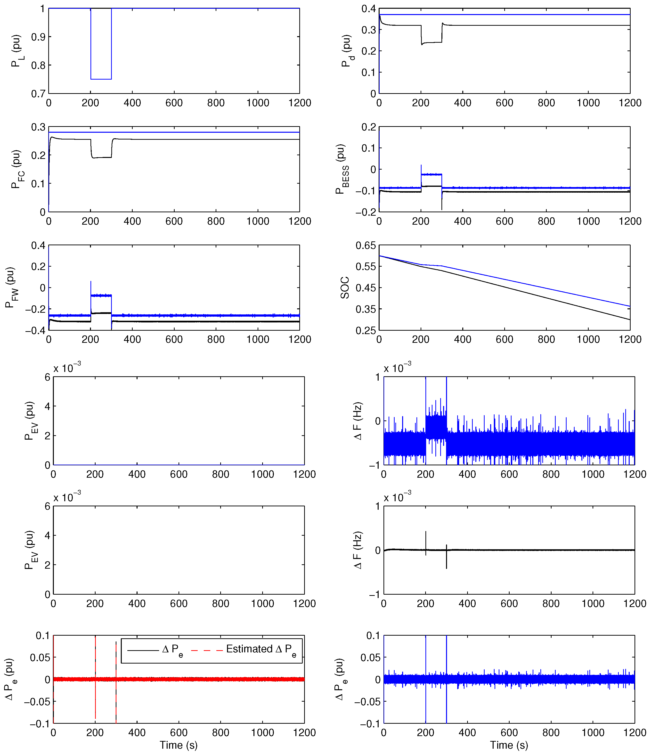
- Base case: At 0 s < t < 200 s, the value of is 1 pu. Therefore, DEG and FC start to feed the power system by their output powers with more amounts than those in the same period of all of the previous cases to compensate the WTG units and PV array outages. Furthermore, BESS and FW begin to release power to the hybrid power system trying to achieve the power balance condition in this severe operating condition. No excess power exists to charge EV in this interval. Simulation results shown in Figure 11 confirm the ability of the proposed control scheme to damp the ΔF and Δ fluctuations with a robust estimate of the full-order observer. On the other hand, for the conventional control approach, DEG and FC produce their maximum limit of power in this period. Therefore, BESS and FW release less power compared to that of the proposed control scheme. Furthermore, there is no excess power to charge EV. However, large fluctuations of ΔF and Δ still appear compared to that of the proposed approach.
- (2)
- Sudden load drop: During 200 s < t < 300 s, suddenly drops from 1 pu to 0.75 pu at t = 200 s. Hence, DEG and FC begin to decrease their output power as the difference between generation and load demand reduces. Furthermore, BESS and FW start to decrease their released power to the system. Though load reduction occurred, there is no surplus power to charge EV in this interval. The control technique keeps ΔF and Δ fluctuations within the acceptable limits. Furthermore, the full-order observer guarantees an effective estimate for Δ, as shown in Figure 11. For the conventional control approach, there is no response for DEG and FC due to the sudden load drop, and they keep producing their maximum limit of power. As a result, BESS and FW continue to decrease their released power in this interval. Furthermore, there is no surplus power to charge EV. Figure 11 shows clearly the fluctuations of ΔF and Δ with using the conventional control scheme in this period.
- (3)
- Sudden load rise: At 300 s < t < 1000 s, suddenly increase from 0.75 pu to 1 pu at t = 300 s. Therefore, the hybrid power system returns safely to the operating condition of the base case. All simulation responses are the same as those in the period 0 s < t < 200 s. Despite these sudden changes and severe operating conditions, the control approach is still capable of holding ΔF and Δ deviations around zero with efficient performance of the observer as indicated in Figure 11. However, the conventional control approach still fails to damp fluctuations of ΔF and Δ in this interval, as shown in Figure 11.
4.5. Case 5
- (1)
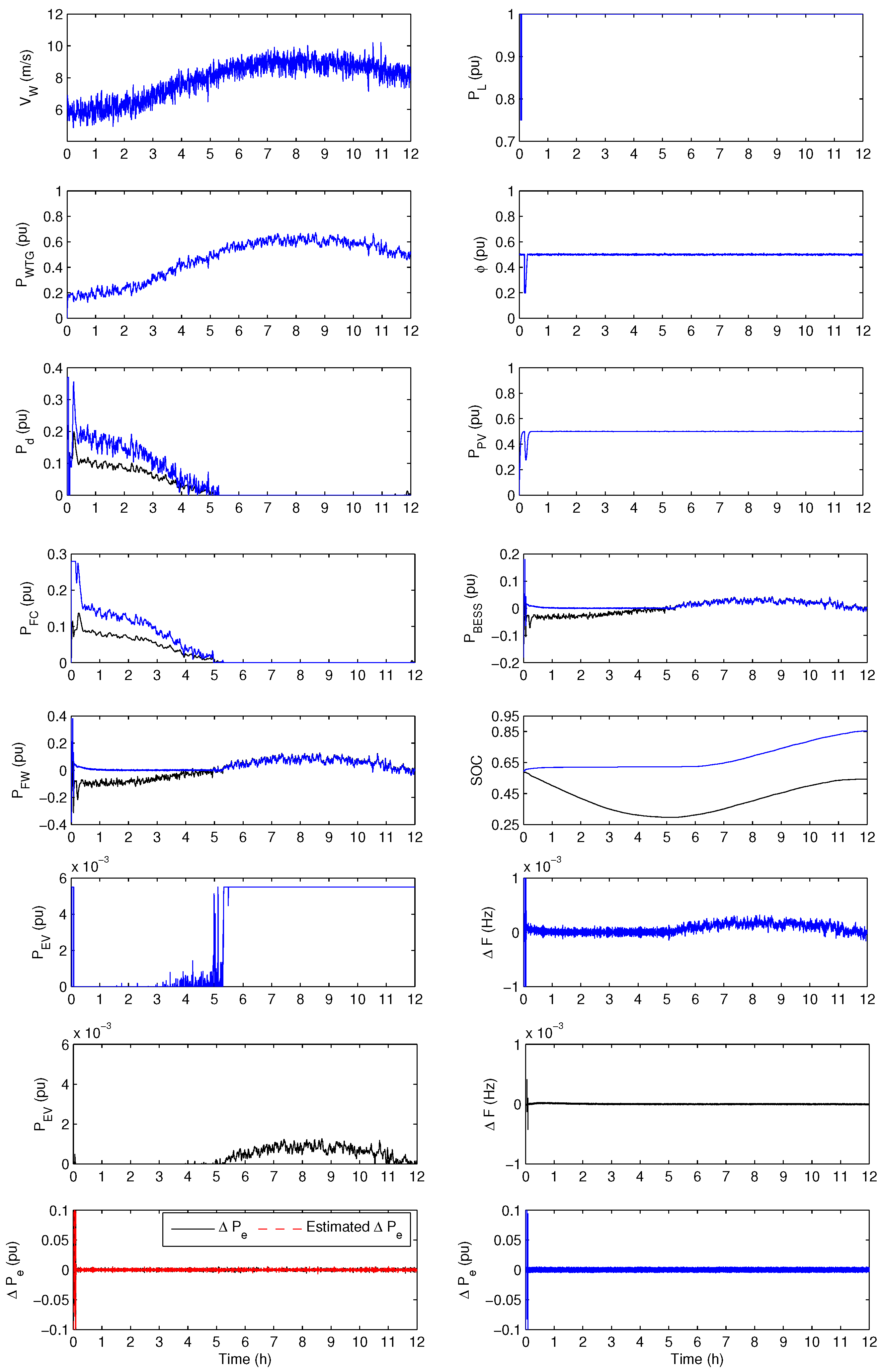
- At 0 h < t < 5 h, starts near 6 m/s and increases till reaching around 8 m/s at t = 5 h. Therefore, begins to rise also from about 0.2 pu to 0.5 pu in the same period. However, with is not sufficient yet to meet the load demand. Hence, DEG and FC are automatically connected to feed the power system with decreasing output power as increases. Furthermore, BESS and FW start to release their power to the system trying to achieve the power balance condition. No surplus power exists to charge EV in this interval. Simulation results clarify that the proposed control scheme can keep ΔF and Δ fluctuations near zero with the effective performance of the proposed full-order observer. For the conventional control approach, DEG and FC produce a larger amount of power with higher overshoot and fluctuations compared to that of the proposed approach. Therefore, BESS and FW decrease their released power in this interval. Clear fluctuations for the charged power of EV, ΔF and Δ compared to the that of the proposed scheme can be noticed in Figure 12 in this period.
- (2)
- When 5 h < t < 9 h, begins to exceed 8 m/s at t = 5 h. At this time, with begins to be enough to meet the load demand. Therefore, DEG and FC are totally disconnected from the system. Furthermore, BESS and FW start to charge the excess power. At the same time, EV begins to store part of the surplus power from the hybrid power system. The proposed control approach still has the ability to damp the ΔF and Δ fluctuations as indicated in Figure 12. Furthermore, the full-order observer ensures robust estimate performance during this period, while higher fluctuations of ΔF and Δ still appear in Figure 12 for using the conventional control approach.
- (3)
- During 9 h < t < 12 h, begins to decrease. Therefore, also starts to drop, but still is sufficient with to feed the load demand. Hence, DEG and FC are still totally disconnected from the power system. BESS, FW and EV begin to reduce their stored power from the hybrid power system as decreases. The proposed control technique succeeded to mitigate ΔF and Δ deviations within the acceptable limits with adequate performance of the full-order observer, as shown in Figure 12. However, the conventional control scheme is still unable to damp the fluctuations of ΔF and Δ compared to the proposed control approach.
5. Conclusions
- (1)
- Control the flow of the output powers of DEG and FC, the stored and released powers of BESS and FW and the charged power of EV at any time according to the variations of wind speed, solar radiation and load demand, so as to suppress the system frequency and supply error fluctuations.
- (2)
- Withstand harsh operating conditions, such as complete shading of the PV array, fast wind speed variation and WTG units and/or PV array outage keeping the system frequency and supply error values within acceptable limits.
- (3)
- Decrease the fluctuations of the energy supply and storage systems (DEG, FC, FW, BESS and EV). Therefore, if this control approach is used, a lesser size of these energy sources will be needed, which improves the overall system efficiency and decreases its cost.
Author Contributions
Conflicts of Interest
References
- Al-Alawi, A.; Al-Alawi, S.; Islam, S. Predictive control of an integrated PV-diesel water and power supply system using an artificial neural network. Renew. Energy 2007, 32, 1426–1439. [Google Scholar] [CrossRef]
- Amin, H.; Maoud, A. Control of hybrid fuel cell/energy storage distributed generation system against voltage sag. Int. J. Electr. Power Energy Syst. 2010, 32, 488–497. [Google Scholar]
- Nander, C. Robust PI control of smart controllable load for frequency stabilization of microgrid power system. Renew. Energy 2013, 56, 16–23. [Google Scholar] [CrossRef]
- Ali, R.; Mohamed, T.; Qudaih, Y.; Mitani, Y. A new load frequency control approach in an isolated small powe systems using cofficient diagram method. Int. J. Electr. Power Energy Syst. 2014, 56, 110–116. [Google Scholar] [CrossRef]
- Howlder, A.; Izumi, Y.; Uehara, A.; Urasaki, N.; Senjyu, T.; Saber, A. A robust H∞ controller based frequency control approach using the wind-battery coordination strategy in a small power system. Int. J. Electr. Power Energy Syst. 2014, 58, 190–198. [Google Scholar] [CrossRef]
- Pan, I.; Das, S. Kriging based surrogate modeling for fractional order control of microgrids. IEEE Trans. Smart Grid 2015, 6, 36–44. [Google Scholar] [CrossRef]
- Lee, D.; Wang, L. Small-signal stability analysis of an autonomous hybrid renewable energy power generation/energy storage system Part I: Time-domain simulations. IEEE Trans. Energy Convers. 2008, 23, 311–320. [Google Scholar] [CrossRef]
- Pahasa, J.; Ngamroo, I. Coordinated control of wind turbine blade pitch angle and PHEVs using MPCs for load frequency control of microgrid. IEEE Syst. J. 2016, 10, 97–105. [Google Scholar] [CrossRef]
- Yang, J.; Zeng, Z.; Tang, Y.; Yan, J.; He, H.; Wu, Y. Load frequency control in isolated micro-grids with electrical vehicles based on multivariable generalized predictive theory. Energies 2015, 8, 2145–2164. [Google Scholar] [CrossRef]
- Zhang, S.; Mishra, Y.; Shahidehpour, M. Fuzzy-logic based frequency controller for wind farms augmented with energy storage systems. IEEE Trans. Power Syst. 2016, 31, 1595–1603. [Google Scholar] [CrossRef]
- Manjarres, P.; Malik, O. Frequency regulation by fuzzy and binary control in a hybrid islanded microgrid. J. Mod. Power Syst. Clean Energy 2015, 3, 429–439. [Google Scholar] [CrossRef]
- Palmer, M.; Tachibana, M.; Senjyu, T.; Funabashi, T.; Saber, A.; Datta, M. Grid stabilization with decentralized controllable loads using fuzzy control and droop characteristics. Int. J. Emerg. Elect. Power Syst. 2014, 15, 357–365. [Google Scholar] [CrossRef]
- Ronilaya, F.; Miyauchi, H. A load frequency control in an off-grid sustainable power system based on a parameter adaptive PID-type fuzzy controller. Int. J. Emerg. Elect. Power Syst. 2014, 15, 429–441. [Google Scholar] [CrossRef]
- Han, Y.; Young, M.; Jain, A.; Zimmerle, D. Robust control for microgrid frequency deviation reduction with attached storage system. IEEE Trans. Smart Grid 2015, 6, 557–565. [Google Scholar] [CrossRef]
- Bevrani, H.; Feizi, M.; Ataee, S. Robust frequency control in an islanded microgrid: H∞ and μ-synthesis approaches. IEEE Trans. Smart Grid 2016, 7, 706–717. [Google Scholar]
- Sekhar, P.; Mishra, S. Storage free smart energy management for frequency control in a diesel-PV-fuel cell-based hybrid ac microgrid. IEEE Trans. Neural Netw. Learn. Syst. 2016, 27, 1657–1671. [Google Scholar] [CrossRef] [PubMed]
- Bevrani, H.; Habibi, F.; Babahajyani, P.; Watanabe, M.; Mitani, Y. Intelligent frequency control in an AC microgrid: Online PSO-based fuzzy tuning approach. IEEE Trans. Smart Grid 2012, 3, 1935–1944. [Google Scholar] [CrossRef]
- Pan, I.; Das, S. Fractional order fuzzy control of hybrid power system with renewable generation using chaotic PSO. ISA Trans. 2016, 62, 19–29. [Google Scholar] [CrossRef] [PubMed]
- Vachirasricirikul, S.; Ngamroo, I. Robust LFC in a smart grid with wind power Penetration by Coordinated V2G Control and Frequency Controller. IEEE Trans. Smart Grid 2014, 5, 371–380. [Google Scholar] [CrossRef]
- Shankar, G.; Mukherjee, V. Load frequency control of an autonomous hybrid power system by quasi-oppositional harmony search algorithm. Int. J. Electr. Power Energy Syst. 2016, 78, 715–734. [Google Scholar] [CrossRef]
- Mi, Y.; Fu, Y.; Li, D.; Wang, C.; Loh, P.; Wang, P. The sliding mode load frequency control for hybrid power system based on disturbance observer. Int. J. Electr. Power Energy Syst. 2016, 74, 446–452. [Google Scholar] [CrossRef]
- Yoshimoto, K.; Nanahara, T.; Koshimizu, G.; Uchida, Y. New method for regulating state-of-charge of a battery in hybrid wind power/battery energy storage system. In Proceedings of the IEEE PES Power Systems Conference and Exposition, Atlanta, GA, USA, 29 October–1 November 2006; pp. 1244–1251.
- Senjyu, T.; Nakaji, T.; Uezato, K.; Funabashi, T. A hybrid power system using alternative energy facilities in isolated island. IEEE Trans. Energy Convers. 2005, 20, 406–414. [Google Scholar] [CrossRef]
- Herrero, J. Non-Linear Robust Identification Using Evolutionary Algorithms. Ph.D. Thesis, Polytechnic University of Valencia, Valencia, Spain, 2006. [Google Scholar]
- Laumanns, M.; Thiele, L.; Deb, K.; Zitzler, E. Combining convergence and diversity in evolutionary multi-objective optimization. Evolut. Comput. 2002, 10, 263–282. [Google Scholar]
- Herrero, J.; Meza, G.; Martinez, M.; Blasco, X.; Sanchis, J. A smart-distributed Pareto front using the ev-MOGA evolutionary algorithm. Int. J. Artifi. Intell. Tools 2014, 23. [Google Scholar] [CrossRef]
- Herrero, J.; Blasco, X.; Martinez, M.; Sanchis, J. Multiobjective tuning of robust PID controllers using evolutionary algorithms. In Lectuer Notes Computer Science; Springer: Berlin, Germany, 2008; pp. 515–524. [Google Scholar]
- Herrero, J.; Blasco, X.; Sanchis, J.; Redondo, J. Design of sound phase diffusers by means of multiobjective optimization approach using ev-MOGA evolutionary algorithm. Struct. Multidiscip. Optim. 2016, 53, 861–879. [Google Scholar] [CrossRef]


| = 0, Speed Regulation R = 2.4 Hz/puMW and K = 500 | M = 0.2 puMW/Hz and D = 0.012 puMW/Hz |
|---|---|
| = 0.1 s and = 2 s | = 1, = 1.85 s, = 0.2 s and = 1/100 |
| = 1 and = 1.5 s | = 1/25, = 0.5 s, = 1/5 and = 4 s |
| = 1/300 and = 0.15 s | = 1/100 and = 0.1 s |
© 2017 by the authors; licensee MDPI, Basel, Switzerland. This article is an open access article distributed under the terms and conditions of the Creative Commons Attribution (CC-BY) license (http://creativecommons.org/licenses/by/4.0/).
Share and Cite
Lotfy, M.E.; Senjyu, T.; Farahat, M.A.-F.; Abdel-Gawad, A.F.; Yona, A. A Frequency Control Approach for Hybrid Power System Using Multi-Objective Optimization. Energies 2017, 10, 80. https://doi.org/10.3390/en10010080
Lotfy ME, Senjyu T, Farahat MA-F, Abdel-Gawad AF, Yona A. A Frequency Control Approach for Hybrid Power System Using Multi-Objective Optimization. Energies. 2017; 10(1):80. https://doi.org/10.3390/en10010080
Chicago/Turabian StyleLotfy, Mohammed Elsayed, Tomonobu Senjyu, Mohammed Abdel-Fattah Farahat, Amal Farouq Abdel-Gawad, and Atsuhi Yona. 2017. "A Frequency Control Approach for Hybrid Power System Using Multi-Objective Optimization" Energies 10, no. 1: 80. https://doi.org/10.3390/en10010080