Numerical Investigation of the Time-Dependent and the Proppant Dominated Stress Shadow Effects in a Transverse Multiple Fracture System and Optimization

Abstract

In this paper, a numerical study is conducted to investigate the stress shadow effects (stress reorientation and change) during hydraulic fracturing in a transverse multiple fracture system. A numerical model is used for the numerical study. It is a 3D model and can simulate the fracture operation from injection begin to full closure (fracture contact). Therefore, there is no need to assume the fracture geometry for the investigation of the stress shadow effects (unlike previous studies). In the numerical study, the first and second operations in a fictive transverse multiple fracture system are simulated, meanwhile the stress shadow effects and their influences on the propagation and proppant placement of the second fracture are investigated. According to the results, the following conclusions are discerned: (1) most proppants are located in the lower part of the reservoir, even below the perforation; (2) the stress shadow effects are time-dependent and proppant dominated; (3) the stress shadow effects affect the fracture propagation and the proppant placement of the second fracture, and also the fracture conductivity of the first fracture; (4) the time-dependent stress shadow effects can be divided into four phases, fracture enlargement, closure without proppant contact, closure with proppant contact and full closure; and (5) the superposition effect of the stress shadow in a transverse multiple fracture system exists. According to the conclusions, some optimizations are recommended.

1. Introduction

Hydraulic fracturing is currently a hot topic in petroleum engineering. It is now the key technology to enhance the gas recovery in tight and shale gas reservoirs, especially when combined with horizontal well bores. During fracturing operations, reservoirs are artificially cracked. With the support of injected solid proppant, a huge highly conductive channel is then created; thus, gas can be economically produced. On the other hand, a horizontal well bore makes it possible to set a fracture cluster in a reservoir; then a large stimulated reservoir volume (SRV) is created.

At present, many researchers focus on the optimization of the transverse multiple fracture system. Meyer et al. [1] developed an analytical solution for predicting the behavior of multiple patterned transverse vertical hydraulic fractures intercepting horizontal wells. Yu and Sepehrnoori [2] used a 2D semi-analytical model to investigate the influences of reservoir permeability, porosity, fracture spacing, fracture half length, fracture conductivity, gas desorption and well spacing on the productivity and the related economic analysis. Later, in Yu and Sepehrnoori [3], the influence of geomechanical effects on the fracture conductivity was further considered. In these 2D models, each fracture in the transverse multiple fracture system has an equivalent geometry (length) and conductivity (aperture), as well as an equivalent fracture spacing to its neighboring fracture. The fracture spacing is not limited, which is unrealistic, especially when the fracture spacing is short, because the influences of the neighboring fractures during fracturing operation are significantly great. In Olson [4], it was found that the fracture spacing and operational sequence (simultaneous, sequential or alternative sequential fracturing) have great influences on the fracture pattern. In a simultaneous operation, the fractures in the middle have normally a shorter length, while, in a sequential operation, the influences of the previous fractures may cause reorientation of the subsequent fractures.

As an optimization concept for the transverse multiple fracture system, man-made fractures with limited reorientation and limited propagation resistance from neighboring fractures are generally preferred, hence, the influences of each fracture on the others must be studied in detail. In fact, the main influence is the stress shadow effect caused by stress changes (magnitude and orientation) due to fracturing operations. The stress shadow effect was first reported in Green et al. [5] and Sneddon et al. [6]. In these publications, the stress distribution of a semi-infinite 2D fracture under constant internal pressure was studied. Soliman and Addams [7] used analytical solutions for a semi-infinite 2D and a penny-shaped fracture to investigate the stress shadow effect of a transverse multiple fracture system. It was found that the stress shadow effect increases with an increasing number of sequential fractures and a decreasing fracture spacing. Cheng [8] used a 2D model based on the boundary element method to analyze the stress distributions around multiple transverse fractures (simultaneously operated) and the geometries of these fractures. It was found that the width profile is no longer elliptic, and the width of the middle fractures is strongly reduced. Nagel and Sanchez-Nagel [9] used commercial software based on the finite difference method and the distinct element method to investigate the stress shadow effect in 3D. The influences of the fracture spacing, rock mechanical properties and in-situ stress ratio were studied. Roussel and Sharma [10] used the same method as that in the work of Nagel and Sanchez-Nagel [9], however, the influence of fracture barriers (cap rock and base rock) was further considered. In that paper, it was found that an alternate fracture sequence (1-3-2-4-5, etc.) is better for creating a multiple fracture system with limited reorientation. Rafiee [11] presented an optimization concept named the modified zipper fracture. The concept is based on the reduction of the stress shadow effect calculated by an analytical solution and a 3D numerical model. In Kresse et al. [12] and Wu et al. [13], a new hydraulic fracturing model for simulating complex fracture network propagation in a formation with pre-existing natural fractures was introduced. The stress shadow effect is calculated using a 2D, plane-strain, displacement discontinuity solution with a 3D correction factor.

Although numerous studies of the stress shadow effect in a transverse multiple fracture system have been reported, there are still some problems. In these studies, an assumed final fracture pattern (semi-infinite or penny-shaped) with an assumed geometry (length, height and width) is generally used to investigate the stress shadow effect, implying that the maximum stress shadow effect has the same depth as the middle point of the fracture. Indeed, the real fracture at the closure stage does not have an ideal geometry even in a homogeneous reservoir because the final proppant distribution dominates the final fracture geometry (Zhou et al. [14]). Due to proppant settling, the propped area below the perforation is normally greater than the area above. Therefore, the magnitude and the shape of the stress shadow effect could be much different than that predicted in the previous studies. Secondly, the stress shadow effect varies from the operation stage to the closure stage.

To the author’s knowledge, there is little information available in the literature about the time dependency of the stress shadow effect and the influences of the proppant placement on the stress shadow effect. The understanding of the changing process is greatly important for the spacing, sequence, as well as operation schedule optimization etc. of a transverse multiple fracture system. The objective of this work is to investigate the temporal variation of the stress shadow effect in consideration of proppant transport and placement. A full 3D numerical model is applied, which can describe not only the fracturing operation process from injection to full closure but also its influences on the surrounding rock formations. According to the results, some optimization concepts are recommended.

2. Theoretical Background

Generally, hydraulic fracturing involves the following main physical processes: mechanical deformation induced by fluid pressure changes in fractures and pores; fluid flow within the fracture and the rock formation, including their interactions; fracture propagation; and proppant transport and settling inside a fracture. In the mathematical model, the rock deformation is described by linear elasticity theory, including the equation of motion (Equation (1)), the continuum equation (Equation (2)) and the constitutive equations (Equations (3) and (4), derived from Darcy law and mass conservation, is used to describe the porous media flow process. The mathematical model of the fracture flow (Equation (5)) is similar to the one for porous media flow. The flow equations for the two processes have the same formulation but different characteristic parameters. In the fracture flow, the conductivity is derived from the simplified Navier–Stokes equation for two parallel plates. For the proppant transport, the mass conservation equation (Equation (6)) is used, in which the settling is implicitly expressed in terms of the proppant velocity. The numerical formulation is described in Appendix A.

$${\sigma }_{ij,j}+\rho (b_i-\frac{d{v}_i}{dt})=0,$$

(1)

$$\Delta {\epsilon }_{ij}=\frac{1}{2}\left(\Delta u_{i,j}+\Delta u_{j,i}\right),$$

(2)

$$\Delta {\sigma }^{\prime }=D\Delta \epsilon ,$$

(3)

$$Q_{leak}+\alpha \frac{\partial e}{\partial t}+\frac{1}{M_b}\frac{\partial P_p}{\partial t}=\nabla \cdot [\frac{K_m}{\mu }\nabla (P_p+{\rho }_{f}gZ)],$$

(4)

$$w(Q_{inje.}-Q_{leak})+\frac{\partial w}{\partial t}=\nabla \cdot [\frac{w^3}{12\mu }\nabla (P_f+{\rho }_{f}gZ)],$$

(5)

$$\frac{\partial (Cw)}{\partial t}+\nabla \cdot (C{v}_{p}w)+w{C}_{inje.}{Q}_{inje.}=0,$$

(6)

where σ = σ′ + αIP_p and σ is the total stress (Pa); ρ is the rock density (kg/m³); b_i is the volumetric acceleration (m/s²); v_i is rock the mass velocity (m/s); Δε is the strain increment (unitless); u is the displacement (m); Δσ′ is effective the stress increment (Pa); α is the Biot coefficient (unitless); I is the unit matrix; D is the physical matrix, i, j ∈ (x,y,z); Q_leak is the leak off rate (1/s); Q_inje. is the fluid injection rate (1/s); K_m is the permeability (m²); e is the volumetric strain (unitless); t is the time (s); M_b is the Biot modulus (Pa); μ is the viscosity (Pa*s); P_p is the pore pressure (Pa); P_f is the fracture pressure (Pa); ρ_f is the fluid density (kg/m³); g is the gravity (m/s²); C is the proppant concentration (%); w is the fracture width (m); v_p is the proppant velocity (m/s); and C_inje. is the proppant injection concentration (unitless).

Most hydraulic fracturing models and commercial software used today, for instance FracPro based on a Pseudo 3D model (Cleary [15] and Cleary et al. [16]), MFrac based on a modified Pseudo 3D model (Meyer [17]) and StimPlan3D based on a Planar 3D model (Peirce et al. [18] and Siebrits et al. [19]) do not consider all of the physical processes mentioned above, e.g., fluid leak off, pore fluid flow, and stress variation in the surrounding rocks. Furthermore, they cannot describe the contact conditions (fracture–fracture contact and fracture–proppant contact) under full fracture closure.

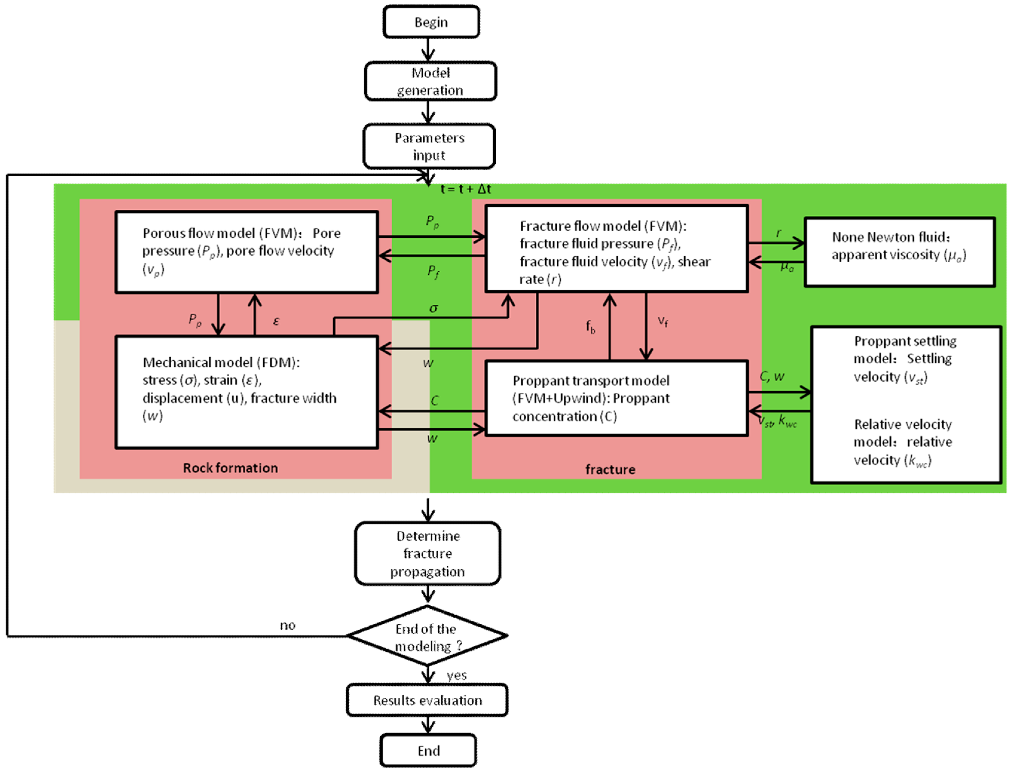
Zhou [14,20] developed a full 3D model based on the governing equations. The simulations of hydraulic fracturing from fracture propagation to full closure (including fracture contact) and proppant transport were verified through comparison of a semi-analytical solution and the results of a proppant transport experiment. Therefore, it can be used to investigate the time-dependent and the proppant dominated stress shadow effect in a transverse multiple fracture system. In the model, these hydro-mechanical coupled equations are numerically solved in a sequential schema (Figure 1), in which the coupling terms have been modified to maintain the conservation of the fluid mass in the fracture. In a computational loop of this method, Equations (4) and (5) are solved independently using the finite volume method at first. In the numerical formulation (Appendix A), the variation of the fracture width in Equation (5) is substituted by a developed constitutive equation (Equation (7)), which describe the aperture variation induced by pressure and stress variation normally acting on the fracture plane Zhou et al. [14]. Then, the fluid pressure and velocity in the fracture and pores as well as the fracture width are estimated. A contact condition is introduced to determine the fracture contact (Equation (7)). If the fracture width is smaller than the given residual width or the proppant concentration is greater than the given maximum value, then the fracture surfaces make contact with either themselves or the proppant, and a contact stress is calculated through the over-reduced fracture width.

$$\Delta w=\frac{P_f(t+1)+{\sigma }_{con}(t)+{\sigma }_n(t)}{{\alpha }_1}{l}_c,$$

(7)

where l_c is characteristic length of a fracture element (m); α₁ = K + 4G/3 is the elastic parameter (MPa); K is bulk modulus (MPa); G is the shear modulus (MPa); σ_n is the normal stress (Pa); σ_con is the contact stress $\{\begin{array}{ll}{\sigma }_{con}(t+1)=0& \mathrm{if}C\le C_{\max }\mathrm{and}w\ge w_{res}\\ {\sigma }_{con}(t+1)={\sigma }_{con}(t)+{\alpha }_1\cdot \Delta {\epsilon }_o& \mathrm{if}C>C_{\max }\mathrm{or}w<w_{res}\end{array}$ (Pa); C_max is the maximum proppant concentration (unitless); w_res is the residual width (m); and Δε_o is the over reduced strain (unitless).

With the calculated fluid velocity, as well as the proppant settling and relative velocity models, the proppant velocity can be computed according Equation (8) (Zhou et al. [14]). Then, the distribution of the proppant concentration can be estimated through solving Equation (6). The final step is the mechanical calculation. After substituting the fracture width and the pore pressure into the mechanical model, the new stress, strain and displacement fields will be computed (see Appendix A).

$$v_p=k_{wc}{v}_l+v_{pst}{c}_{corr}{w}_{corr}\cos \theta =k_{wc}{v}_l+v_{ps}\cos \theta ,$$

(8)

where v_l is the liquid velocity (m/s), v_p is the proppant velocity (m/s), k_wc is the relative velocity coefficient (unitless), v_pst is the corrected Stoke’s settling velocity for a single particle (m/s), c_corr is the influence factor of proppant concentration (unitless), and w_corr is the influence factor of well retardation (unitless).

3. Numerical Investigation

In this paper, we conduct a numerical study of a fictive transverse multiple fracture system. The main objective is to investigate the influence of time and proppant distribution on the stress shadow effect. Therefore, other influence factors such as rock mechanical properties and in-situ stress ratio are not concerned.

3.1. Modelgeneration

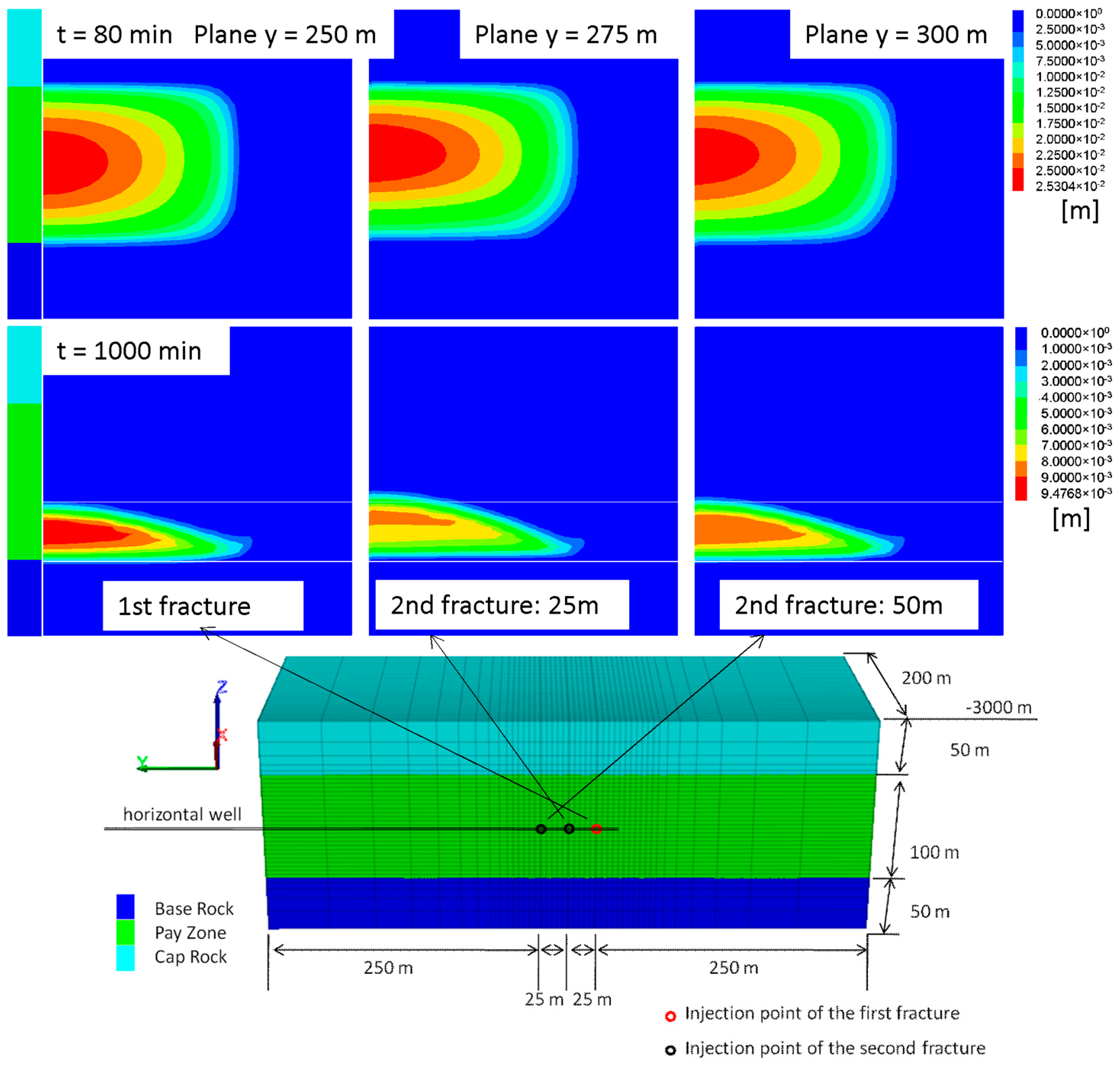
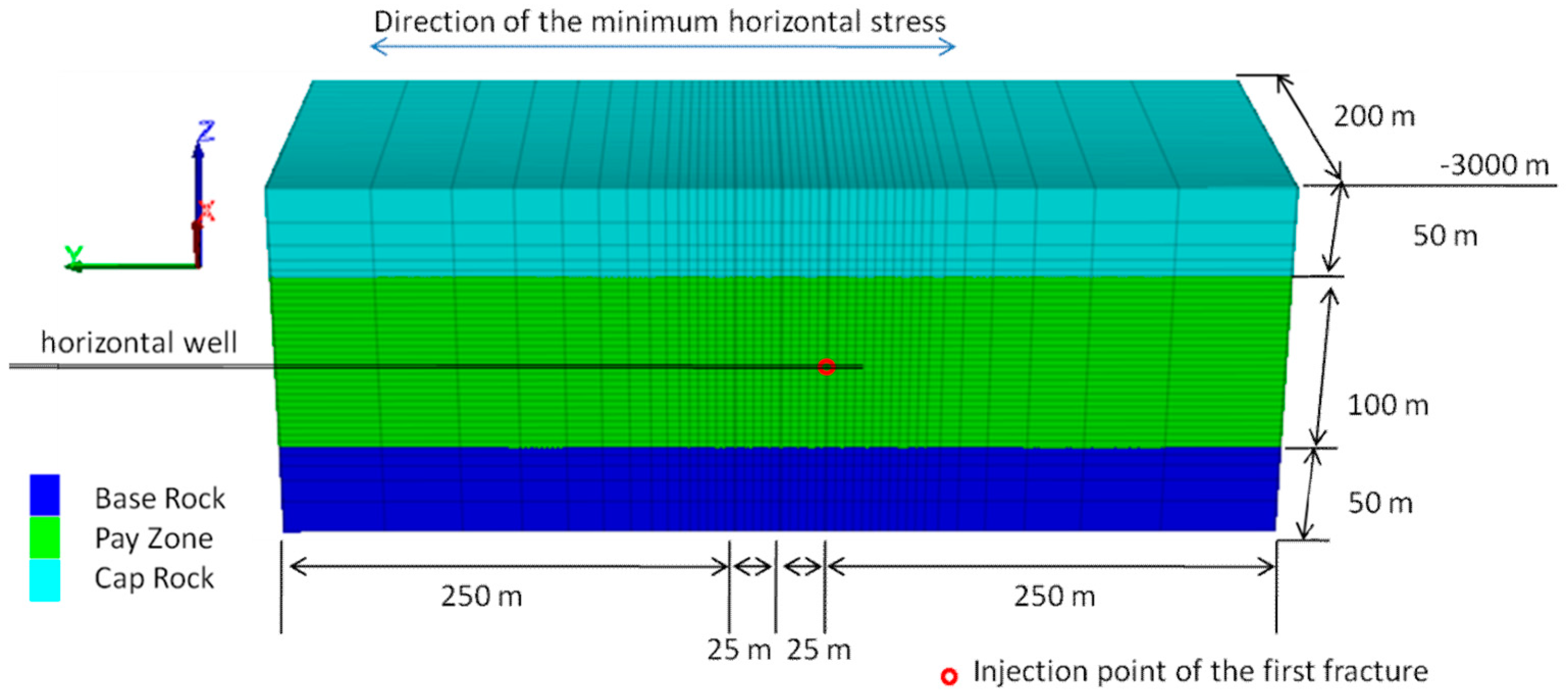
A half reservoir model is generated and illustrated in Figure 2. It has a geometry of 200 m (x) × 550 m (y) × 200 m (z) and consists of three horizontal layers: cap rock, pay zone and base rock. The mechanical and hydraulic properties of each layer are listed in

Table 1. Mechanical and hydraulic properties of the rock formations in the calculation model.

Rock Formation	Rock Density (ρ) (kg/m3)	Young’s Modulus (E) (GPa)	Poisson Ratio (υ) (unitless)	Tensile Strength (σt) (MPa)	Porosity (φ) (unitless)	Permeability (Km) (m2)
Cap Rock	2600	25	0.3	1.0	0.025	1 × 10−17
Pay Zone	2600	30	0.25	1.0	0.1	1 × 10−15
Base Rock	2600	25	0.3	1.0	0.025	1 × 10−17

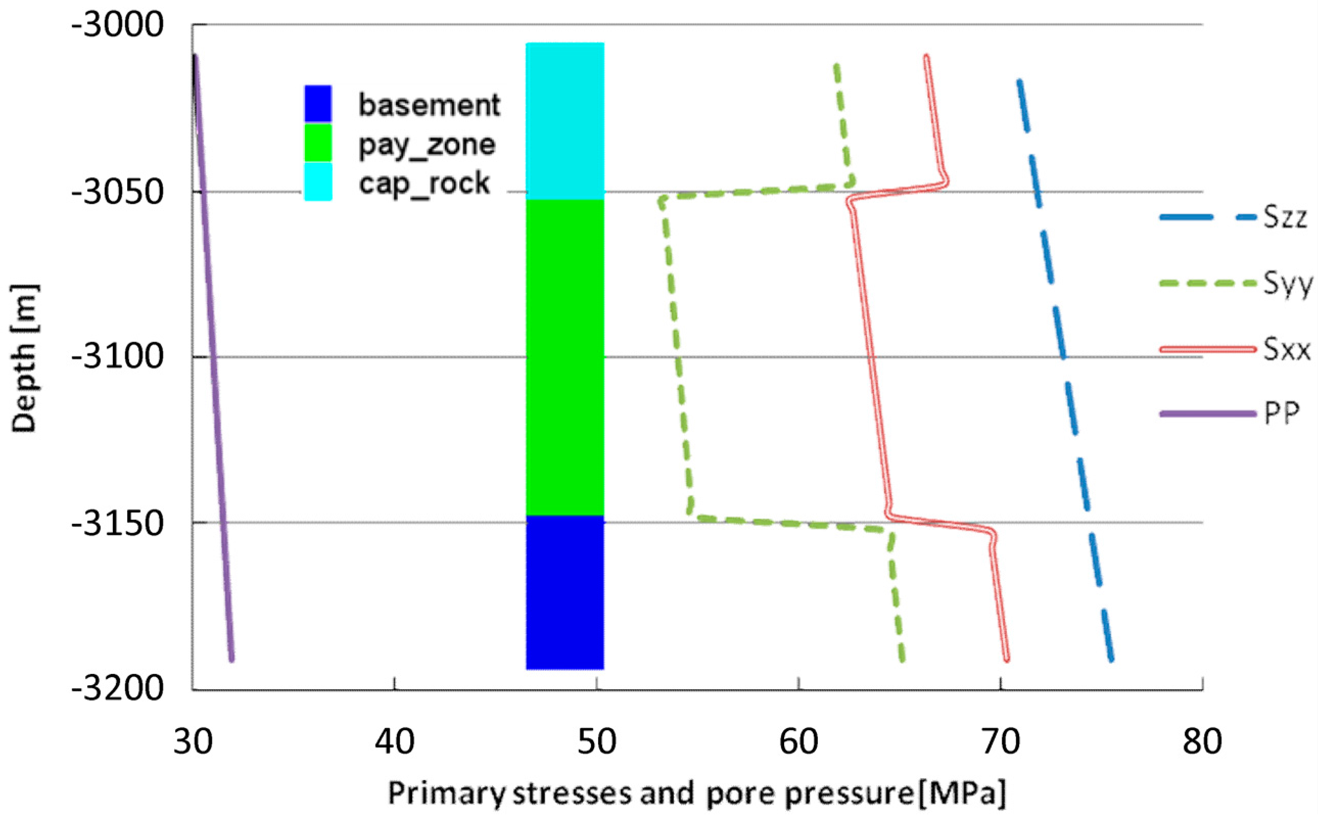
. Figure 3 shows the primary stress and pore pressure. The direction of the minimum horizontal stress is the same as that of the y-axis. A horizontal well is drilled through the middle part of the model and along the direction of the minimum horizontal stress, indicating a transverse multiple fracture system.

3.2. Numerical Results of the First Fracturing Operation

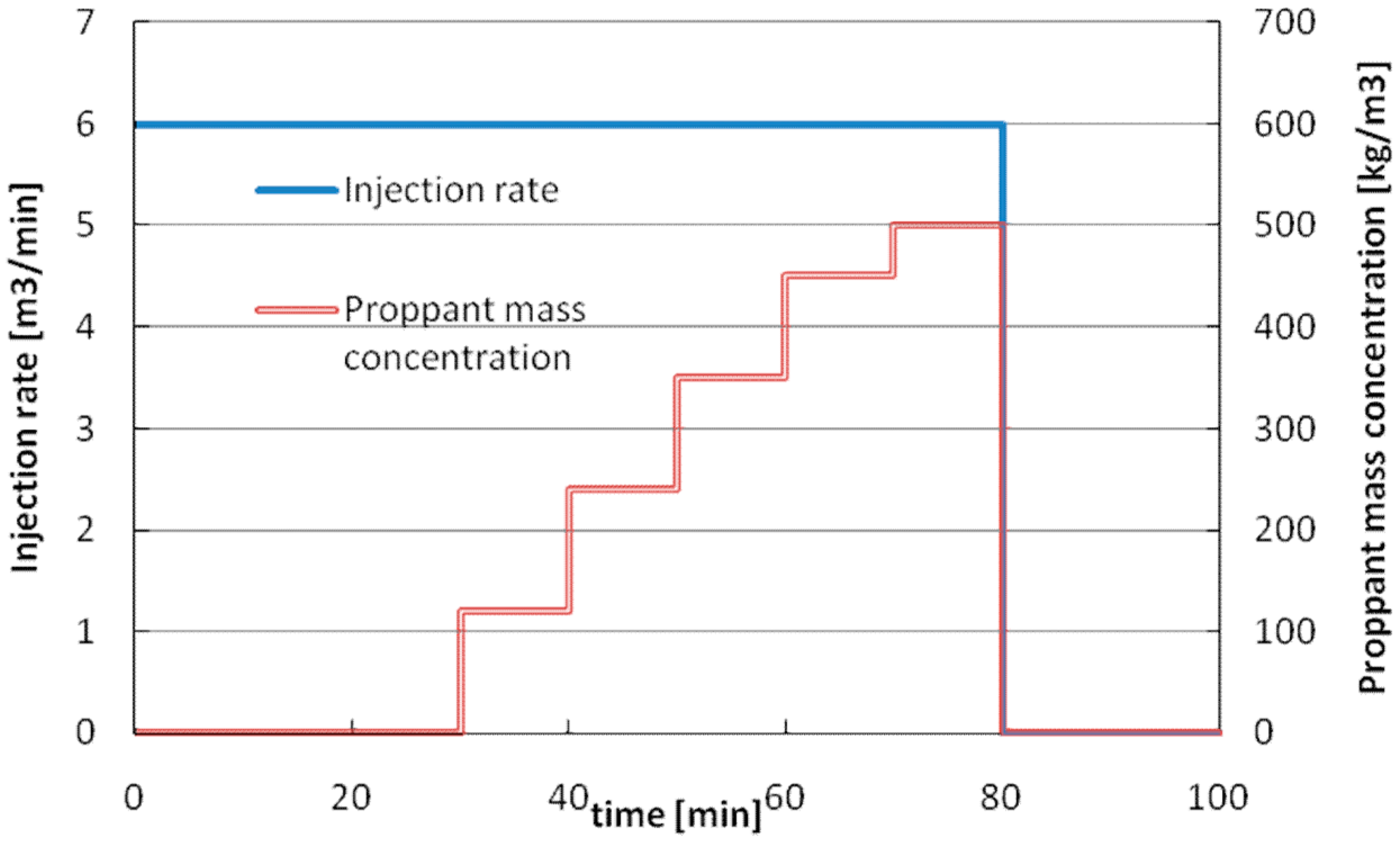
The first injection position (0, 250, −3100) is set 300 m away from the left side of the reservoir model (Figure 2). An 80 min operation with an injection rate of 6 m³/min is designed. At t = 30 min, proppant is added with a stepwise increasing concentration from 0 to 500 kg/m³ (Figure 4). The properties of the fluid and proppant are listed in

Table 2. Fluid and proppant parameters.

Parameters	Symbol	Unit	Values
Proppant density	ρp	kg/m3	3500
Fluid density	ρf	kg/m3	1040
Fluid viscosity	μl	Pa∙s	0.1
Proppant diameter	dp	mm	0.667
Power law coefficient	n	-	1
Parameter for viscosity correction	a	-	1.8
Maximum proppant concentration	Cmax	-	0.65

.

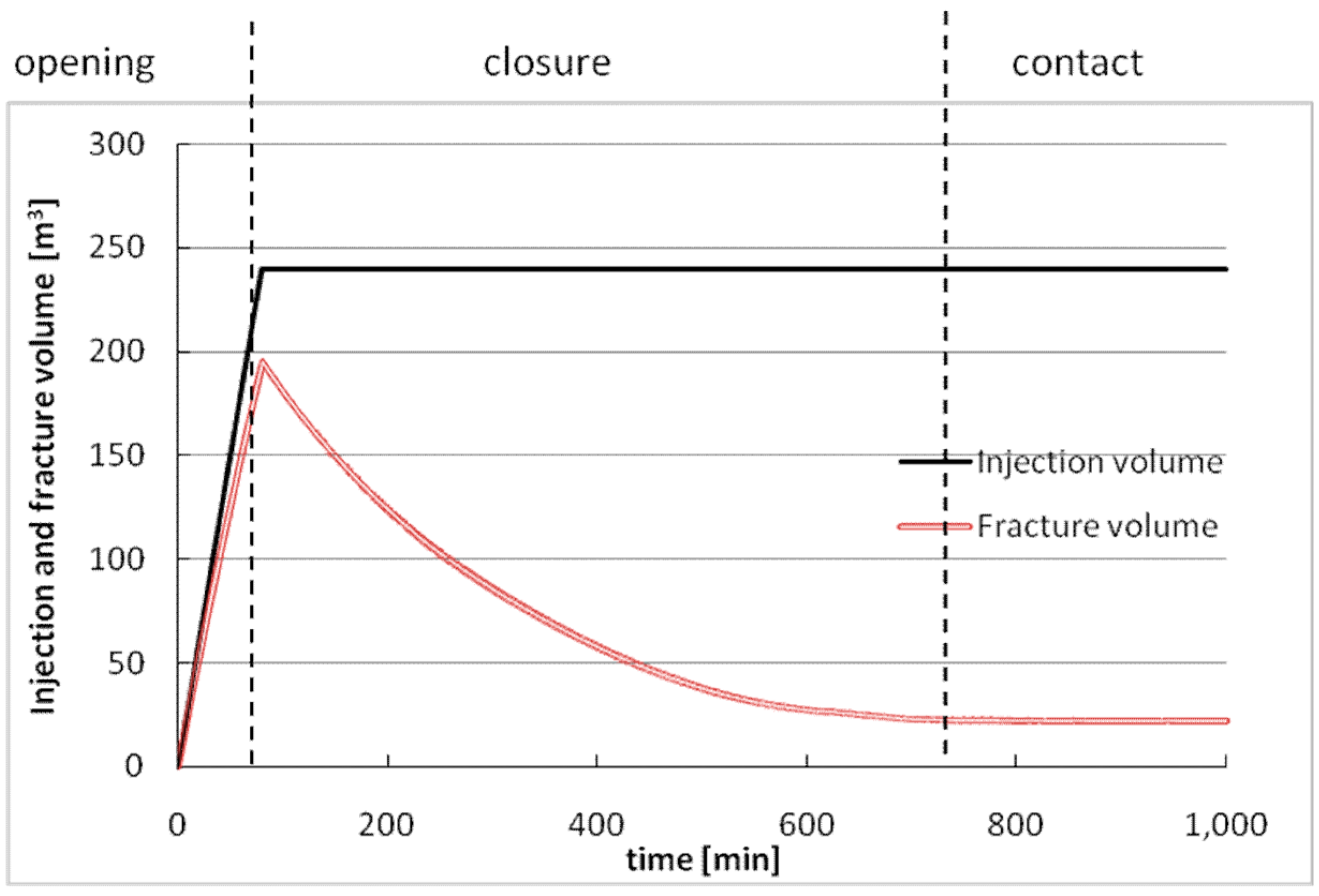
Figure 5 shows the temporal development of the fracture and injection volumes. The difference between them is the leak off volume. During the injection phase, the fracture volume increases linearly, then decreases from 80 min to ca. 710 min with a decreasing rate, and finally remains constant, indicating that the final proppant placement and full fracture closure are achieved after that time.

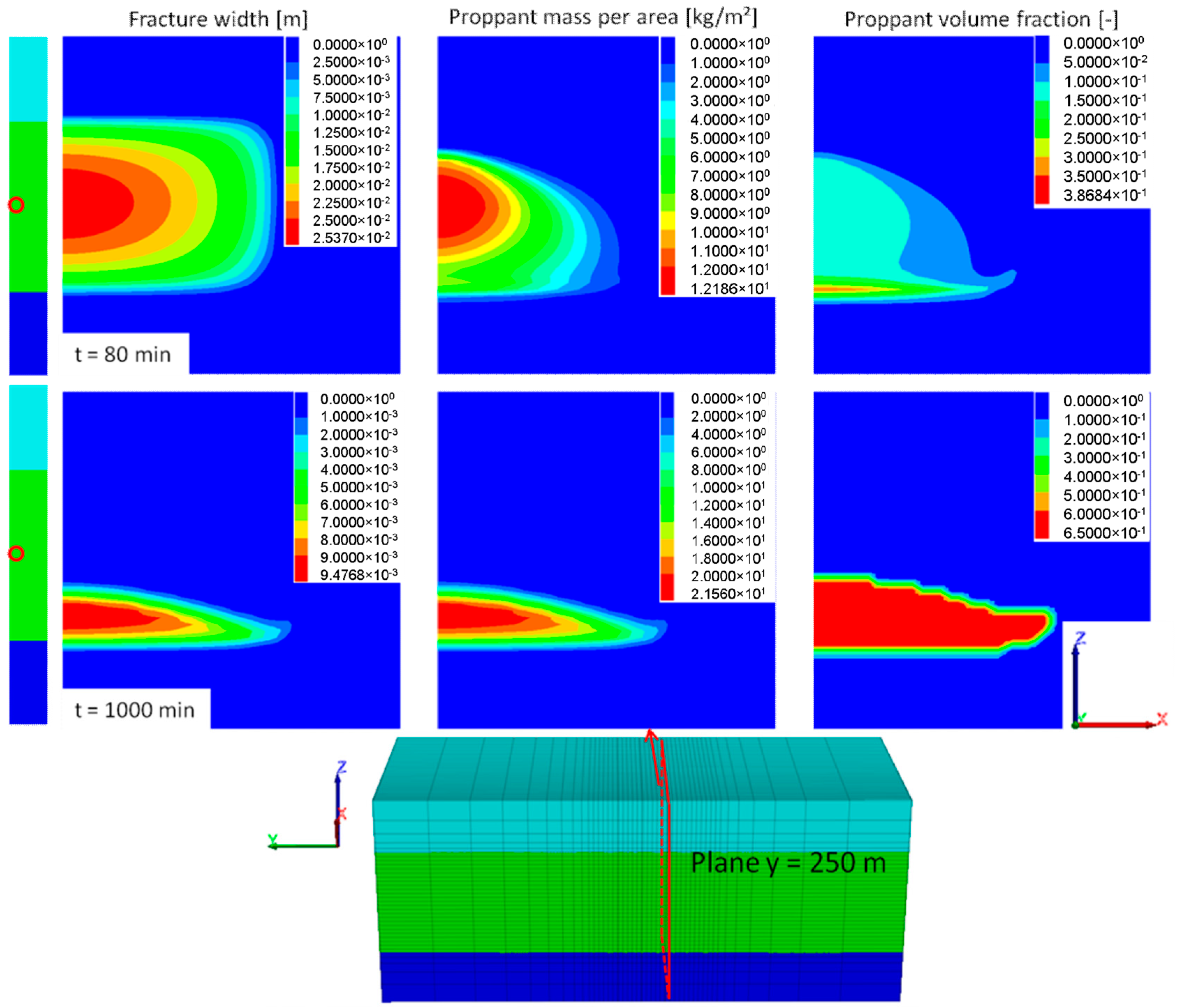
Figure 6 shows the fracture geometry in terms of the width contour, the distribution of the proppant mass per area and the proppant volume fraction. At t = 80 min, the fracture geometry is almost regular and limited between the top and the bottom barriers, which have much higher closure stress. The maximum width is located at the perforation. Unlike the fracture geometry, the proppant has an irregular distribution due to the settling effect. At t = 1000 min (920 min after shut in), the fracture width and the proppant mass per area have the same contour distribution, implying that the magnitude of the fracture width and the area of the propped fracture after full closure are dominated by the proppant placement. The maximum width is reduced from 2.53 cm to 0.95 cm and its position is 34 m deeper than the perforation. The (half) effective fracture area is also reduced from 14,998 m² to 4196 m².

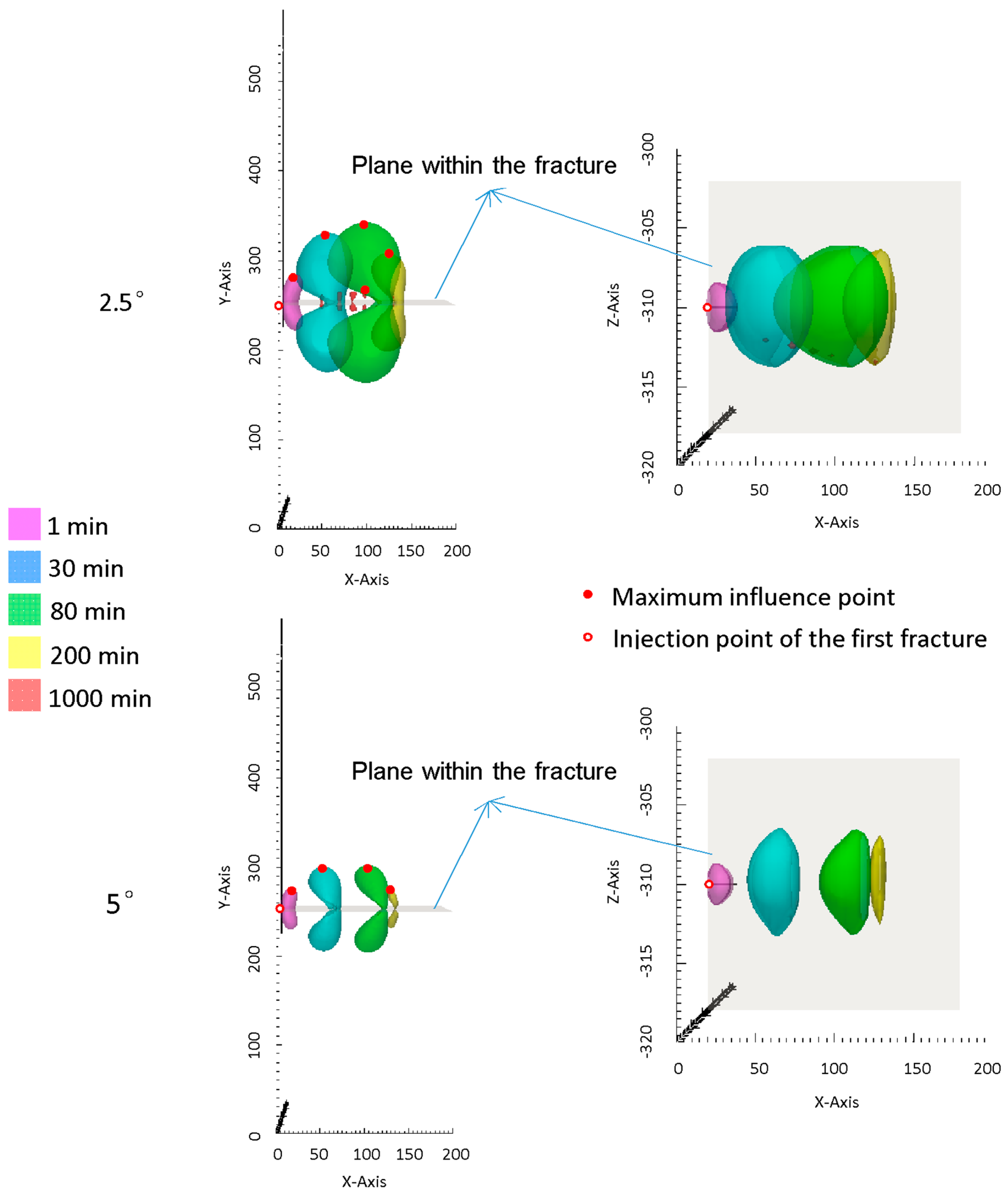
Figure 7 shows the spatial contour of the minimum horizontal stress with 2.5° and 5° reorientations at different time. The contour has two symmetric wings and its shape changes with time. In general, the shape of the contour enlarges during the injection and shrinks after shut in. At t = 1000 min, the contour with 5° reorientation disappears. For a transverse multiple fracture system, the maximum influence point of the stress reorientation with a certain grade is defined as the point on the contour furthest to the fracture plane (Figure 7). In general, its projection point is inside the created fracture (except t = 1 min).

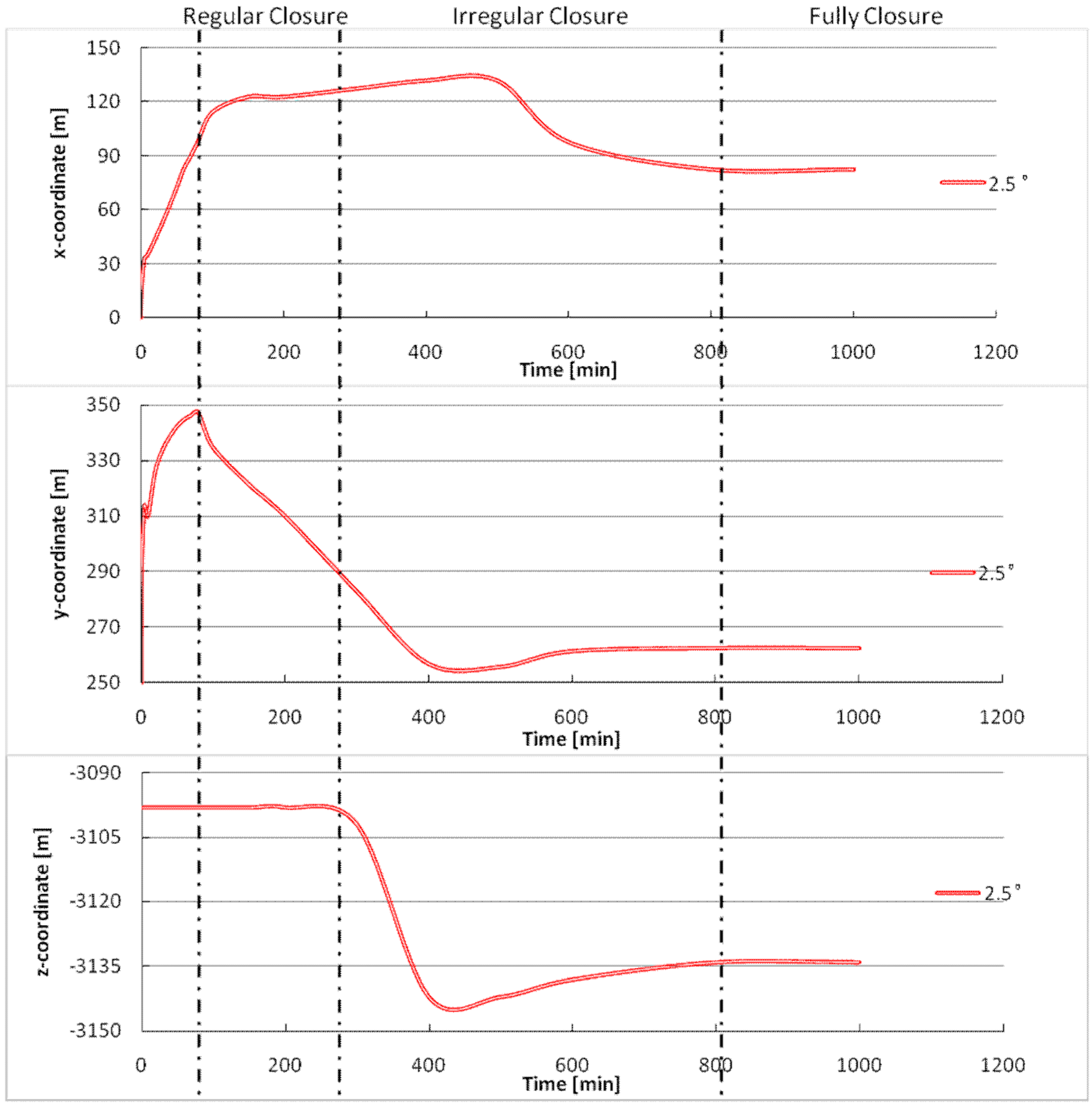
The position of the maximum influence point with a 2.5° stress reorientation varies with time. Figure 8 shows its temporal development. The x-coordinate increases quickly during the injection and slowly during the first 420 min after shut in (till 500 min). The tendency is similar to that of the fracture propagation (fast propagation during injection and slow post-propagation after shut in). Then, it decreases until full closure. The decrease is due to the full closure of the front region, where no proppant is placed. The y-coordinate also increases during the injection, decreases after shut in (from ca. 300 m to 262.5 m) and remains unchanged after full closure. The tendency is similar to that of the fracture volume (Figure 5), indicating that the y-coordinate of the maximum influence point is strongly dependent on the created fracture volume. The z-coordinate remains unchanged before t = 300 min because the fracture has an enlargement and closure without influence of proppant until that time. Then, it decreases rapidly followed by a slight increase. The final z-coordinate is 34 m below the perforation because of the irregular fracture closure due to the proppant redistribution and placement. As a result of the settling effect, the proppant is located in the lower part of the fracture. It prevents the created fracture from fully closing. Conversely, the upper part without proppant can be fully closed. When the proppant in the lower part contacts with the fracture, closure with proppant contact occurs.

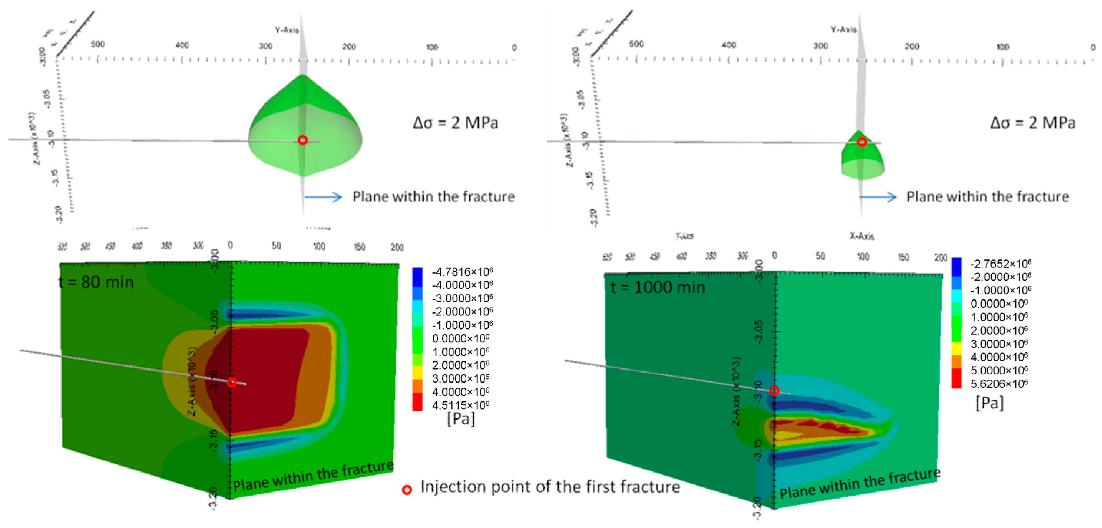
Figure 9 shows the change of the minimum horizontal stress at t = 80 min and 1000 min. In general, the stresses increase in the region perpendicular to the opened fracture and, meanwhile, decrease outside the fracture front. The contour shape of the stress increase (i.e., 2 MPa in Figure 9) is similar to a cone whose bottom is perpendicular to the fracture plane. The cone-like contour shrinks during the closure process, implying that the influence decreases.

3.3. Numerical Results of the Second Fracturing Operation after Full Closure of the First Fracture

In a transverse multiple fracture system, the previous fracture may cause new fractures to deviate from the trajectory of the previous fracture. A minimum fracture spacing to ensue transverse multiple fracture growth is desirable for efficient gas production. To avoid strong direction deviations, a minimum fracture spacing must be characterized, i.e., the distance from the maximum influence point with a 2.5° stress reorientation to the previous fracture represents the minimum fracture spacing with a fracture reorientation smaller than 2.5°.

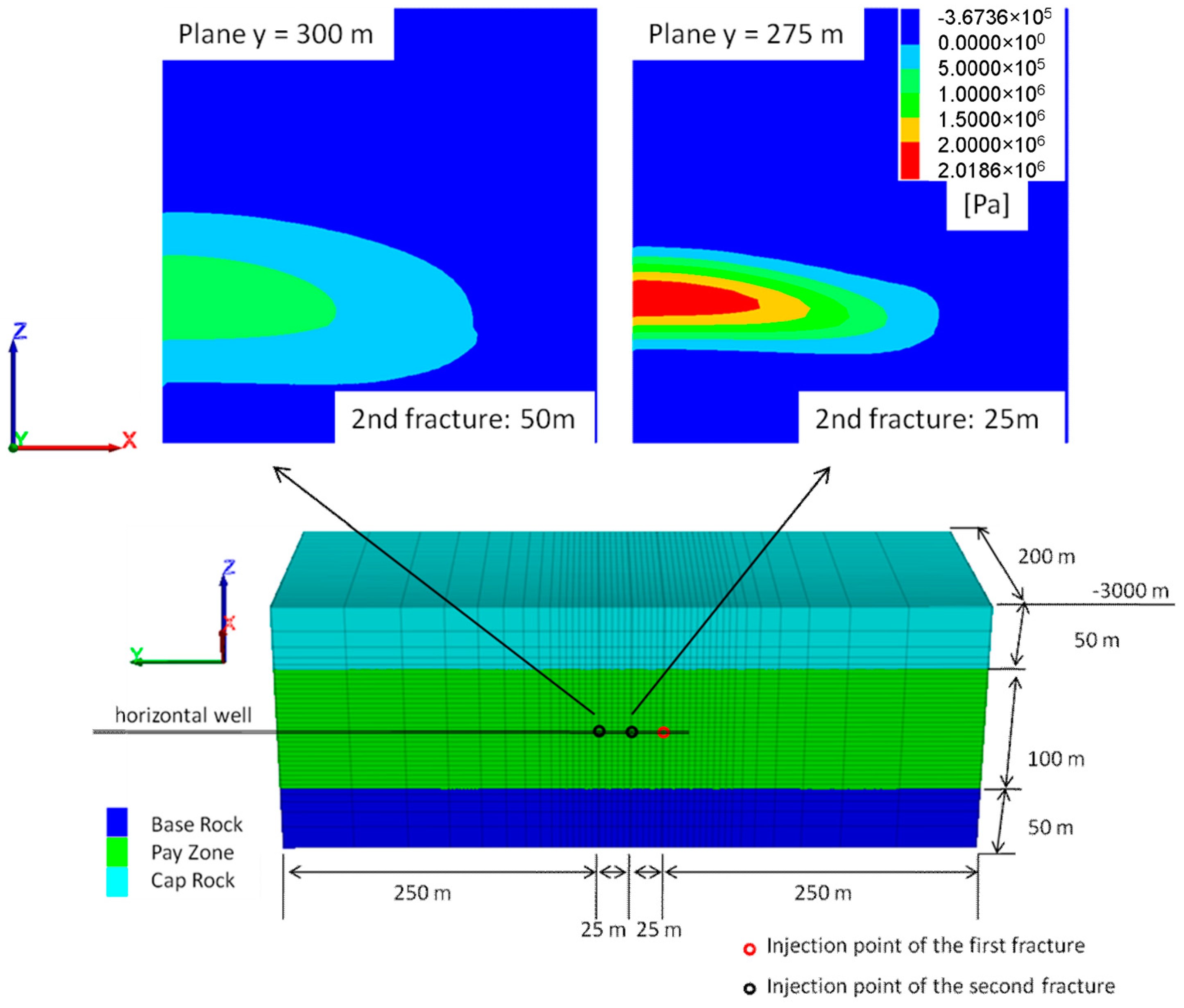
Two fracture spacings (25 m and 50 m) are chosen to investigate the influences of the stress shadow effect on the second operation. The maximum stress reorientation on the plane with 25 m and 50 m spacing are 1.5° and 0.8°, respectively. Due to the small stress reorientation and for simplification, the propagation direction of the second fracture is assumed to be parallel to that of the first operation. The stress shadow effect is then the change of the minimum horizontal stress shown in Figure 10.

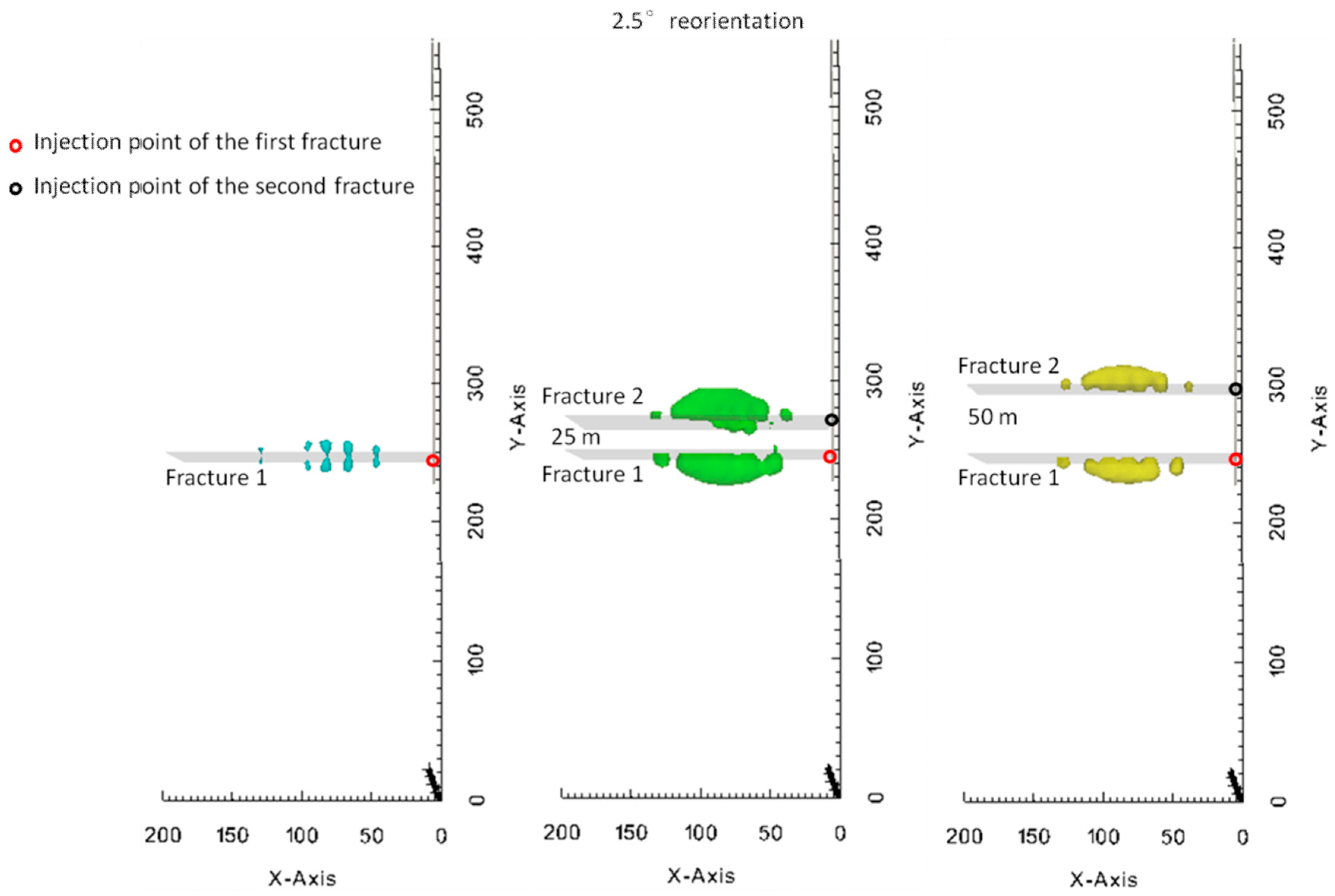
Figure 11 shows the comparison of the fracture propagation before shut in and the propped fracture after final closure of the first and the second operations. Although the created fracture areas are similar, the propagation of the second fracture before shut in becomes irregular due to the stress shadow effect. The lower part has a smaller propagation rate and a smaller fracture width than the upper part because the minimum horizontal stress increased in the lower part and decreased in the upper part (Figure 10). This is more obvious with the 25 m fracture spacing because the stress change is greater. The finial fracture patterns are also similar, but they have different areas and width distributions (Figure 11). In general, the propped area increases (

Table 3. Comparison of the fracture and the propped area of the first and the second operations.

	First Operation	Second Operation: Spacing 25 m	Second Operation: Spacing 50 m
Fracture area (m2)	14,998	15,006	15,016
Propped area (m2)	4196	4349	4367

), the width decreases and its distribution becomes uniform, and the final fracture pattern shifts upward. Due to the stress shadow effect, the lower part of the second fracture has a higher closure stress and a smaller fracture width, which leads to the reduction of the proppant settling, the acceleration of the fracture closure in the lower part and finally upward-shift of the proppant location. The upward-shift effect decreases with increasing fracture spacing (25 m spacing with a 10 m upward-shift and 50 m spacing with a 4 m upward-shift).

Figure 12 shows the comparison of the spatial contours with a 2.5° stress reorientation of the first and the second operation after full closure. In general, the stress reorientation effect between the two fracture planes (inside the fracture system) is strongly reduced (25 m) or even disappears (50 m); conversely, its range of the influence on both sides of the fracture system increases. The results can be explained by the superposition principle: between the two fractures, the stress reorientation effect from the two fractures has opposite directions, whereas it has the same direction outside the fractures. The distance from the maximum influence point to the fracture plane increases from 12.5 m to 24.5 m and 20.1 m for the 25 m and 50 m spacings, respectively.

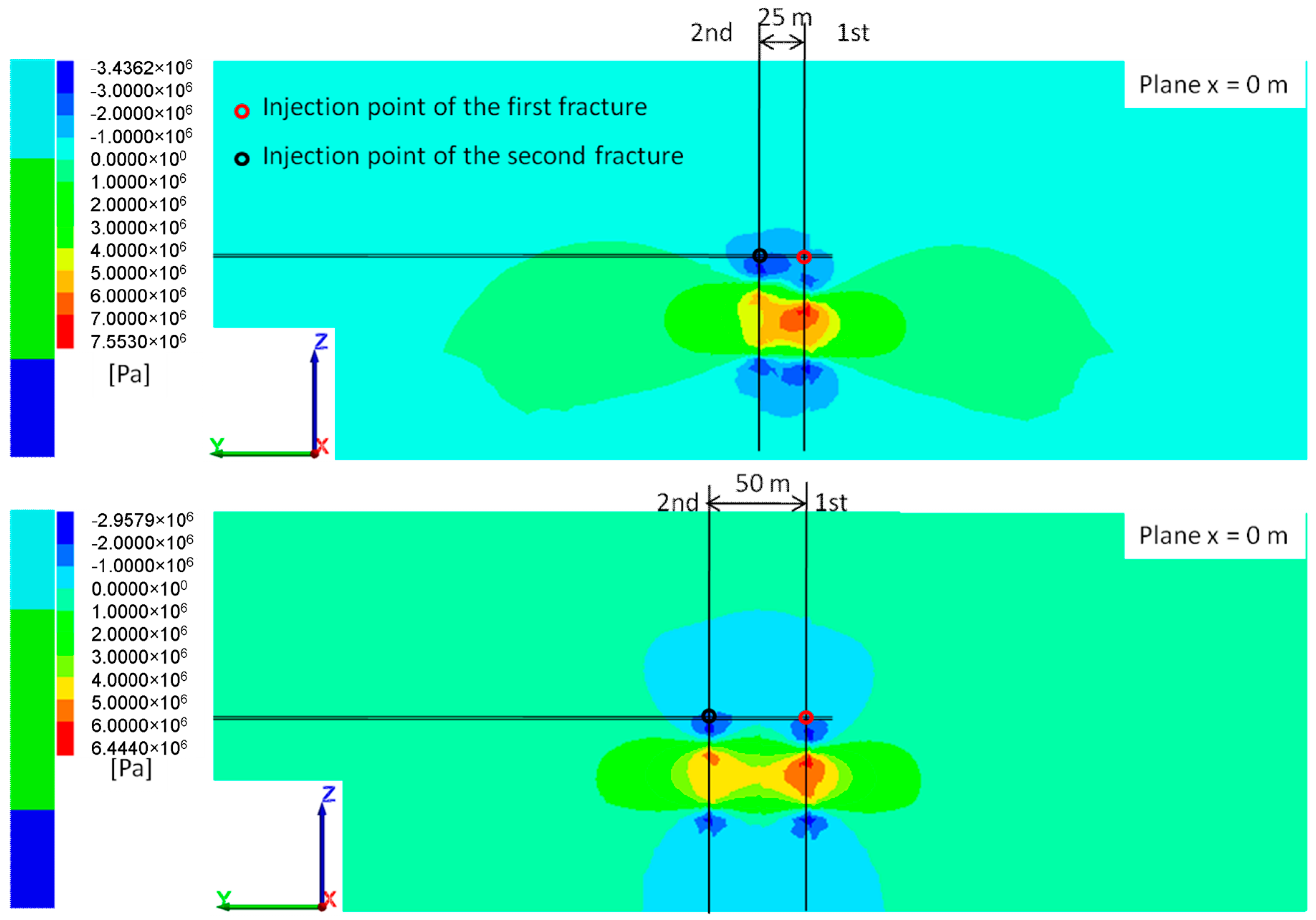
Figure 13 shows the change of the minimum horizontal stress after fully closure of the second fracture. The contour changes from asymmetric to symmetric with increasing fracture spacing. The minimum horizontal stress increases due to the superposition effect. The maximum change is on the first fracture plane. It increases from 5.82 MPa to 7.55 MPa and 6.44 MPa for 25 m and 50 m spacings, respectively, indicating that the created conductivity of the first fracture can also be influenced by the second fracture (conductivity reduction caused by increasing contact stress).

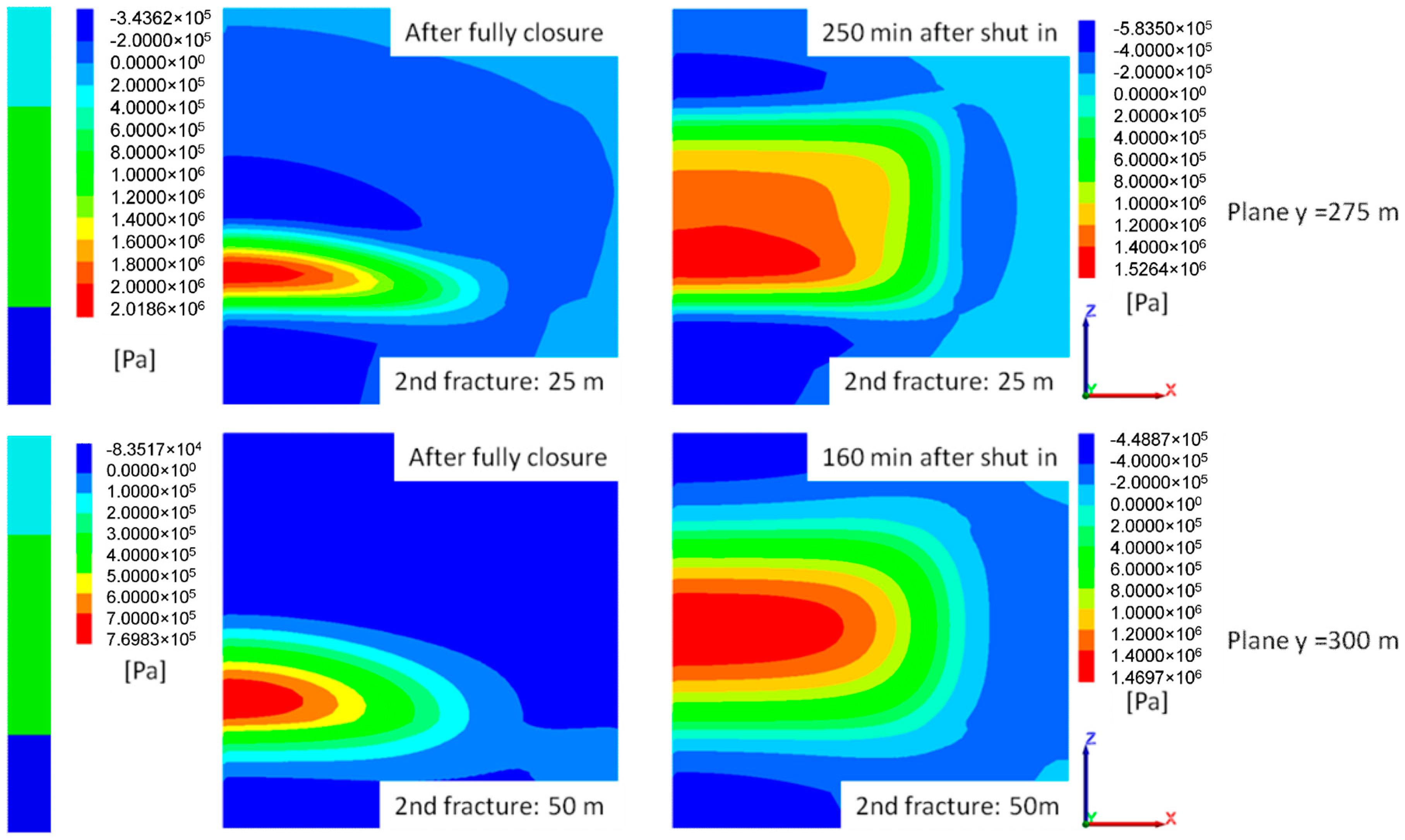
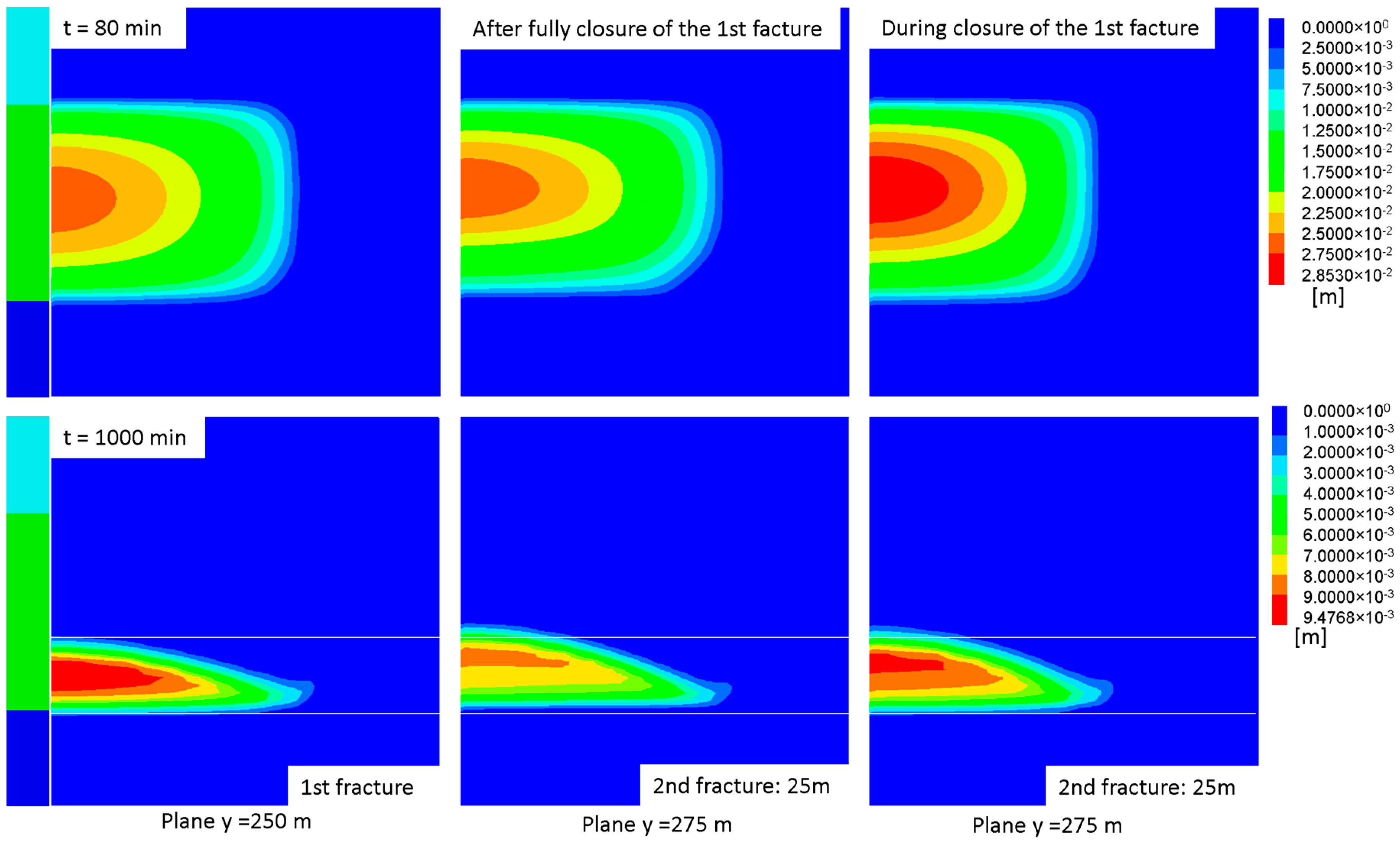
3.4. Numerical Results of the Second Fracturing Operation during Closure Process of the First Fracture

According to the results of the first operation, the stress shadow effect is time dependent. If the second fracturing operation starts during the closure process of the first fracture, then the stress shadow effect dynamically influences the second fracture. In this study, the second operation with a 25 m and 50 m spacing is set to start 250 min and 160 min after closure of the first fracture, respectively. After these times, the stress reorientation on the plane of the second fracture is smaller than 2.5° (Figure 8), which ensures a transverse multiple fracture system.

The changes of the minimum horizontal stress on the fracture plane for the 25 m and 50 m spacing are shown in Figure 14. The stress change during the closure process of the first fracture is different from the one after full closure. In general, the stress in the whole pay-zone increases. The maximum stress increase for both is ca. 15 MPa. As mentioned in Section 3.2, the first fracture begins to irregularly close after 300 min (220 min after shut in). Therefore, the stress change at t = 240 min (160 min after shut in) seems to be regular, and at t = 330 min (250 min after shut in), it seems to be irregular.

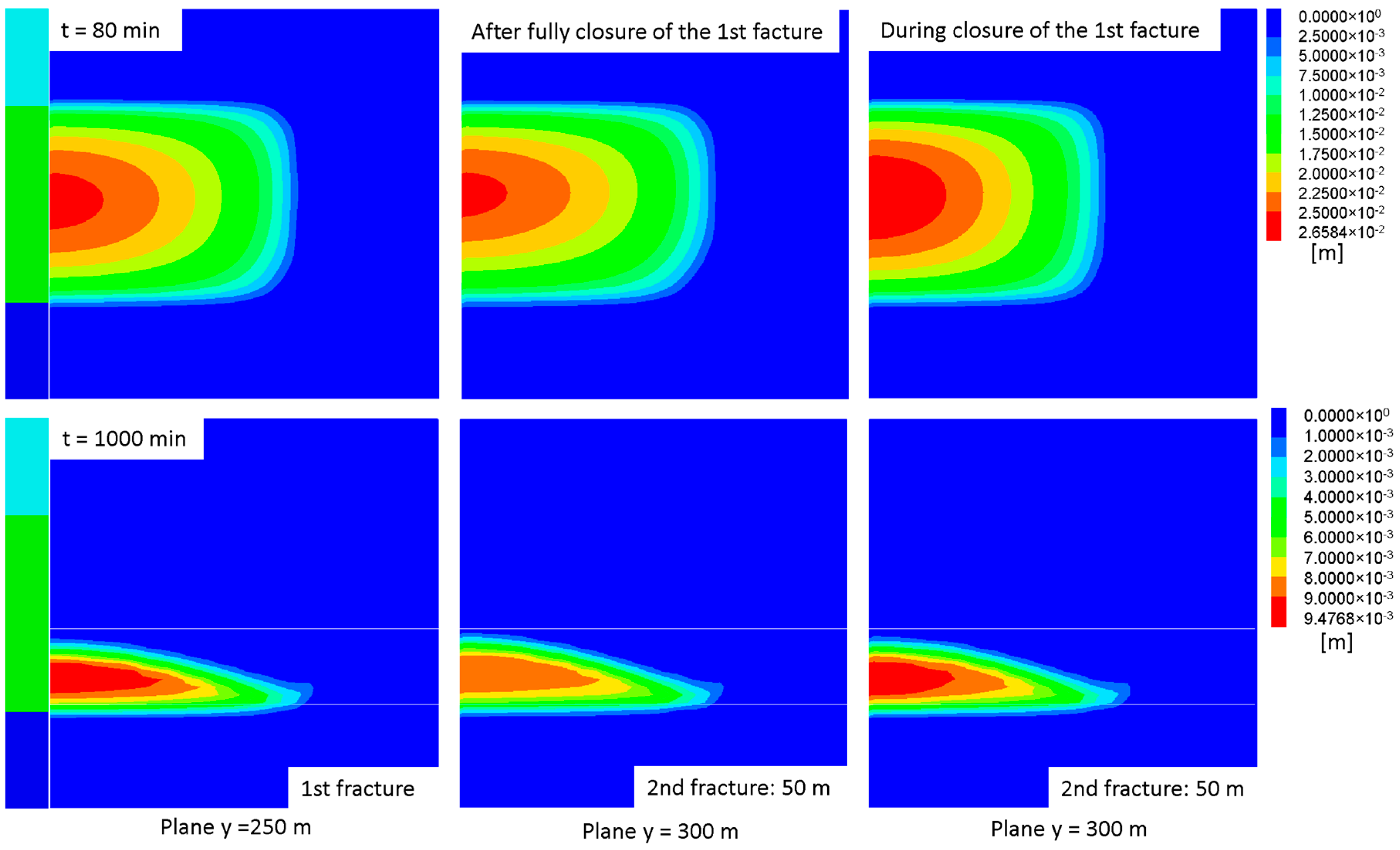
Figure 15 and Figure 16 show comparisons of the fracture propagation before shut in and the propped fracture after final closure of the first and the second operations with 25 m and 50 m spacings, respectively. The time dependent influences of the stress shadow effect are clearly obtained. In general, the fracture propagation is hindered due to the increasing minimum horizontal stress in the whole pay zone. The finial fracture area for 25 m and 50 m spacings are 13,622 m² and 14,598 m² (

Table 4. Comparison of the fracture and the propped area after full closure and during the closure process.

	First Operation	Second Operation: Spacing 25 m (after Fully Closure)	Second Operation: Spacing 25 m (250 min after Shut In)	Second Operation: Spacing 50 m (after Fully Closure)	Second Operation: Spacing 50 m (160 min after Shut In)
Fracture area (m2)	14,998	15,006	13,622	15,016	14,598
Propped area (m2)	4196	4349	4364	4367	4173

), respectively, which are smaller than those of the second operation after full closure of the first fracture. The hindering effect decreases with increasing spacing. The width contour also changes. Due to the hindering effect, a high fluid pressure is needed for fracture propagation, which leads to an increase of the fracture width.

The propped areas of the cases differ. With the 25 m spacing, the propped area did not change significantly. Although the length is shorter due to the hindering effect, the height is greater. The growth in the height occurs mainly in the lower part of the proppant placement. This is due to the higher settling velocity caused by the increasing fracture width. With the 50 m spacing, the propped area is less than that of the second operation after full closure of the first fracture, but the fracture pattern and area are similar to those of the first fracture, indicating that the stress shadow effect does not have a significant influence.

4. Discussion

Through the numerical investigation of the hydraulic fracturing in a fictive reservoir, the following results are obtained:

• Both the final fracture width and the final fracture conductivity are dominated by the final proppant placement. Although the created fracture appears to be regular, the propped fracture is irregular. In general, the upper part of the created fracture is difficult to prop, and the proppant is concentrated in the lower part due to the proppant transport and settling effects.
• The stress shadow effect (stress reorientation and change) varies with time. Its range enlarges during the injection and shrinks during the closure process. The range depends on the fracture width distribution. Therefore, it is also dominated by the proppant placement after final closure. The maximum influence point moves firstly along with the fracture front and away from the fracture plane during the injection. Then, it moves backward to the fracture plane and the propped fracture tip during the closure process; meanwhile, it moves down to a location even below the perforation due to the placement of the proppant at the bottom of the fracture.
• The stress shadow effect affects the fracture propagation and the proppant placement of the second fracture. The influences depend on the time and the fracture spacing. In general, the stress shadow effect decreases with increasing spacing. The time dependent influence can be divided into four time periods: fracture enlargement, closure without proppant contact, closure with proppant contact and full closure. These periods can be determined by the position trajectory of the maximum influence point with a certain reorientation grade.
• After full closure, the second fracture propagates more in the upper part of the reservoir. The final fracture and propped area increase, whereas the width decreases and its distribution becomes uniform. The fracture pattern shifts upward. During closure without proppant contact, the fracture propagation is strongly hindered, which causes both an increase of the fracture width and the settling effect. Therefore, there is little upward-shift effect, and the propped fracture length as well as the propped area may be reduced. The influences of the stress shadow effect during closure with proppant contact are between those without proppant contact and after full closure.
• Due to the superposition principle, the stress reorientation effect between the two fractures is reduced or even disappears, whereas it increases on both sides of the fracture system. Conversely, the change of the minimum horizontal stress also increases, especially between the two factures. The second fracture also has influences on the first fracture in the form of a conductivity reduction caused by increased contact stress on the proppant in the first fracture.

Based on these results, the following optimizations are recommended:

• Because of the settling effect, most proppant is located in the lower part of the reservoir. Therefore, it is better to drill the horizontal bore in the lower part of the reservoir, whereby a good connectivity between the perforation and the propped fracture will be created. The precondition is that the lower barrier must have enough resistance to prevent the fracture from going through, especially for a thin pay zone.
• The spacing optimization of the transverse multiple fracture is mainly based on the stress shadow effect (stress reorientation and change). In general, a minimum spacing must be determined, that will not result in any strong reorientation (i.e., 5° in Roussel et al. [10]) or great increase of the contact stress on the previous fractures.
• In a sequential transverse multiple fracture system, the next operation is preferred to begin after full closure of the previous fracture because the area of the hydraulic fracture and the propped fracture are greater, and the fracture width becomes uniform.
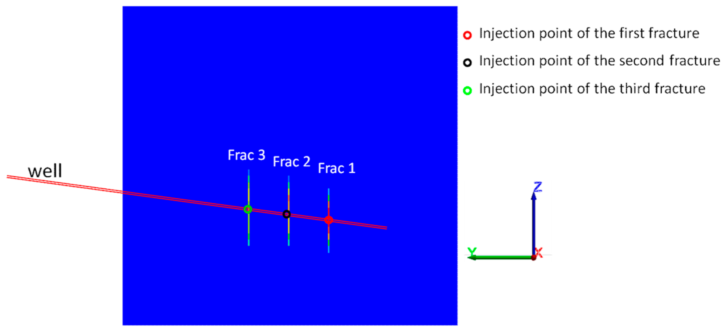
• Regarding proppant transport in boreholes, a horizontal borehole with a small inclination is better than one with no inclination because the gravitational force is positive. In a sequential transverse multiple fracture system, the upward-shift effect plays a positive role for an inclined borehole (Figure 17). The trajectory of the horizontal bore can be optimized according to the calculated fracture pattern.
• If the reservoir is thin and the fracture spacing is short; then the upward-shift and the superposition effect will reduce the resistance of the upper barrier; thus, it may lose its function as a height control. To avoid this situation, a suitable spacing must be designed because the upward-shift effect decreases with increasing spacing.
• In a simultaneous multiple fracture system, the propagation of each fracture will be hindered because the stress shadow effect during the injection is greatly stronger than after full closure. To minimize the stress shadow effect, the designed spacing is generally greater than that of a sequential system. This indicates that a simultaneous multiple fracture system can save operation time, but the fracture number must be reduced.
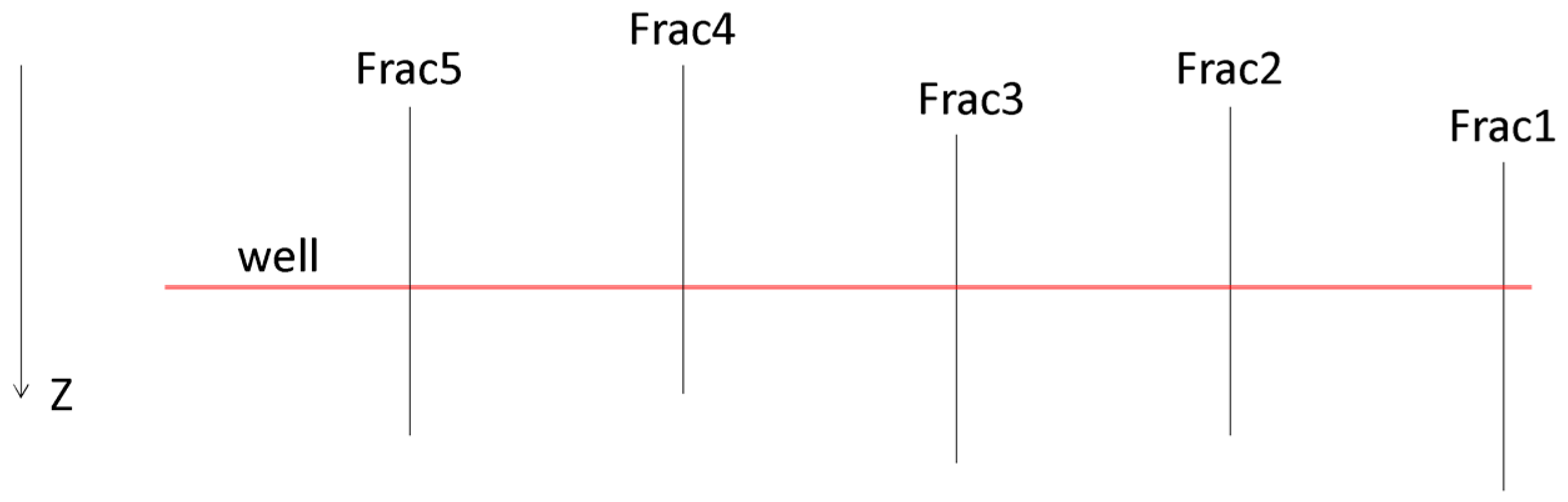
• An alternative fracture sequence (1-3-2, etc.) is recommended in Roussel et al. [10]. With this sequence, the stress reorientation between the first und the third fracture is minimized as shown in Figure 12. Therefore, there is no reorientation problem for the second fracture, and, thus, the fractures can be placed much closer to each other. However, the stress change must also be considered. There are two problems with such an alternative sequence. One is the increasing stress on the second fracture plane. It hinders the propagation of the second fracture in the horizontal direction and may cause a loss of height control when the reservoir is thin and the stress difference between the pay zone and the barrier is small. On the other hand, it is difficult for a horizontal well to cross the middle part of each fracture due to the double upward-shift effect (Figure 18).

The stress shadow effects contain stress reorientation and variation. In this paper, the temporal development of the stress shadow effects during the operation and after shut in was investigated in detail. As the developed simulator is limited only for fractures with the orientation perpendicular to the minimum horizontal stress, it is not possible to simulate the fracture reorientation due to stress changes. In fact, a 3D model for simulation of arbitrary propagation during hydraulic fracturing is still a challenge. The arbitrary reorientation was already realized in 2D models, e.g., the model developed by Kresse et al. [21] based on the DDM theory. In Kresse et al. [21], a simultaneous multiple fracture operation was modeled. On both sides, a small reorientation was observed. The reorientation is probably due to the small stress anisotropy (1.4 MPa), which is not normal, especially for a deep reservoir. Zhou et al. [22] developed a 2D model using the XFEM theory. In his study, the fracture reorientation does not seem to be significant. On the other hand, the effect of stress variation is great both in Kresse and Zhou’s simulation. In this study, it was also found that the fracture propagation and proppant placement are strongly influenced by the stress variation depending on the fracture geometry of the previous fracture. In future work, efforts should be paid to develop a more realistic 3D model considering fracture reorientation, thus the 3D reorientation effect can be studied.

5. Conclusions

In this paper, a numerical study was conducted to investigate the time dependency of the stress shadow effect and the influences of the proppant placement on the stress shadow effect. According to the study, the following conclusions are discerned: (1) The magnitude and range of the stress shadow effect varies with variation of the fracture width. The variation of the fracture width has four phases, enlargement, closure without proppant contact, closure with proppant contact and full closure, revealing that the stress shadow effect is time-dependent; (2) The closure with proppant contact and full closure phases is influenced by proppant transport and placement, implying that the stress shadow effect is proppant dominated in that two phases; (3) The stress shadow effects affect the fracture propagation and the proppant placement of the next fracture, and also the fracture conductivity of the previous fracture; (4) The superposition effect of the stress shadow in a transverse multiple fracture system exists. According to the conclusions, some optimizations are recommended (Section 4).