The Economy-Carbon Nexus in China: A Multi-Regional Input-Output Analysis of the Influence of Sectoral and Regional Development

Abstract

China has become the world’s largest carbon dioxide (CO₂) emitter. Sectoral production activities promote economic development while also adding considerably to national CO₂ emissions. Due to their different sectoral structures, each region shows different levels of economic development and CO₂ emissions. The Chinese government hopes to achieve the dual objectives of economic growth and CO₂ emissions reduction by encouraging those sectors that have high economic influence and low environmental influence. Based on the above background, this study constructed an inter-regional sectoral economic influence coefficient (REIC) and a CO₂ emissions influence coefficient (RCIC) based on the basic multi-regional input-output (MRIO) model to analyse the economy-carbon nexus of 17 sectors in 30 regions in China in 2010. The results showed that most Chinese sectors and regions had low CO₂ emissions influences in 2010. However, some sectors showed negative environmental influences. Specifically, the mining-related sectors showed high CO₂ emissions influence with low economic influence. It is encouraging that some light industry and high-end equipment manufacturing sectors had low CO₂ emissions influence with high economic influence. For regions, geographic location and past preferential policies are the most important factors influencing local economic growth and CO₂ emissions reduction. Most inland regions have low economic influence with high or low CO₂ emissions influence. Meanwhile, most coastal regions showed high economic influence with low CO₂ emissions influence. Finally, we propose some policy implications for sectors and regions.

1. Introduction

The greenhouse effect is considered one of today’s most important global environmental issues. CO₂ emissions from fossil fuel combustion are believed to be the most important factor contributing to greenhouse gas (GHG) and are responsible for over 60% of this deleterious effect [1]. China has now become the world’s largest CO₂ emitter [2,3,4,5,6,7]. In 2015, China’s CO₂ emission was 9.125 billion tons, accounting for 27.2% of the world's total emission [8]. In 2015, at the 21st Conference of the Parties to the United Nations Framework Convention on Climate Change, the Chinese government declared that China would strive to fulfil its commitment to reaching peak CO₂ emissions by approximately 2030, by which point it also aims to reduce its CO₂ emissions per unit of GDP by 60% to 65% of its 2005 level [9]. Sectoral production plays a leading role in China’s CO₂ emissions [10]. This is because production activities consume large amounts of energy and because China's energy consumption primarily depends on coal and other fossil fuels [11]. Specifically, more than half of China’s CO₂ emissions come from the combustion of fossil fuels [12].

The production sector’s CO₂ emissions are closely related to its energy consumption structure. Sectors with high fossil energy intensity, such as electricity production, transportation and steel production, generate far higher CO₂ emissions than sectors with low fossil energy intensity, such as agriculture and services [13,14,15,16,17,18].The electricity production sector accounted for the largest share (47.2%) of China’s CO₂ emissions in 2002 [13]. Additionally, the transportation and steel production sectors are also considered highly fossil energy-intensive. For example, the transportation sector accounted for approximately 62% of total national CO₂ emissions in the United States in 2015, as 63.2% of that sector’s energy consumption relied on fossil oil [16,19]. It is important to recognize that, in different countries, the use of renewable energy resources can lead to different levels of reduction in CO₂ emissions. In Brazil, CO₂ emissions will be reduced by 20% by 2020 due to the increased use of bio-ethanol and biodiesel in the transportation sector [17,18,19]. Moreover, Germany’s CO₂ emissions (31 million tons) are half of Korea’s (66 million tons) despite similar production levels because steel production in Germany uses the electric furnace route, which relies on renewable energy, while steel production in Korea uses the blast furnace route, which depends heavily on fossil fuel [20,21]. Compared to highly energy-intensive sectors, the agricultural sector and the services sector are considered low-carbon production sectors because little fossil fuel is used in their production processes [22,23]. However, some studies have indicated that China’s service sector is a high CO₂ emitter because its electricity is produced mostly from coal [24].

Because different sectors have different CO₂ emissions, the combined structures of different sectors in regions lead to different regional CO₂ emissions [25]. According to the Energy Information Administration, CO₂ emissions in countries that are members of the Organization for Economic Cooperation and Development (OECD) versus emissions in non-OECD countries were 12,867 million tons and 20,671 million tons in 2015, respectively [8]. CO₂ emissions in the non-OECD countries were double those of OECD countries. Most non-OECD countries, such as China and India, are developing countries and are pursuing economic growth that is heavily dependent on sectors with high fossil energy intensity sectors [26,27]. In China, total national CO₂ emissions were estimated at 8673 million tons, and energy-intensive sectors accounted for 80.91% of these emissions in 2010 [28]. Moreover, the Central region was the largest CO₂ emitter among China’s 8 regions (Northeast region, North Municipalities region, North Coast region, East Coast region, Central region, Northwest region and Southwest region) [13]. After China, India is the third largest CO₂ emitter in the world [2,29,30], and the CO₂ emissions of five energy-intensive sectors (iron and steel; cement; chemicals and petrochemicals; pulp and paper; and aluminium) accounted for 56% of its total CO₂ emissions in 2010 [29,30,31,32].

The single-region input-output (SRIO) model is a widely used approach to estimating sectoral CO₂ emissions because it allows the tracing of both direct and indirect CO₂ emissions in a single sector. Several studies have used an SRIO model to analyse CO₂ emission for sectors in a single region [33,34,35,36]. However, with the development of interregional and international trade, it is necessary to extend the scope of analysis from a single region to more regions. Thus, the multi-regional input–output (MRIO) model has been widely used for this purpose [37,38,39,40,41,42,43,44,45,46,47]. Especially since China became the world’s largest CO₂ emitter, more and more researchers have adopted the MRIO model to study the country’s CO₂ emissions flows at interregional and international levels [12,13,48,49,50,51]. Feng et al. [12] and Su and Ang [49] studied CO₂ emissions flows at both interregional and international levels by using the full MRIO approach and the hybrid model, respectively. Furthermore, at the international level, Su and Thomson [52] and Su and Ang [53] studied how different assumptions regarding exports and imports affect CO₂ emissions, respectively.Su and Thomson [52] found that the emission intensity in processing exports is much smaller than those in normal exports when estimating China’s CO₂ emissions. Su and Ang [53] estimated China’s CO₂ emissions with two different methods, and got two different outcomes; the competitive imports assumption gave a larger estimate than the non-competitive import assumption.

This study provides a theoretical framework to support policy-making for economic development and CO₂ reduction at the sectoral and regional levels. Specifically, we constructed two coefficients (REIC and RCIC) based on the MRIO model to capture the benchmarking sectors and regions with high economic influence and low CO₂ emissions influence in China. Moreover, based on these two coefficients, we propose policy implications for these sectors and regions to help the Chinese government achieve the dual objectives of economic growth and CO₂ emissions reduction. The paper proceeds as follows. In Section 2, we describe the methodology and data used to examine sectoral influences on the economy and CO₂ emissions. In Section 3, we present the results from the perspectives of sectors and regions. Finally, Section 4 concludes the study and provides policy implications.

2. Methodology and Data

2.1. Methodology

This study develops a methodology based on the MRIO model. We construct the REICs and RCICs of China’s 17 sectors in 30 regions in 2010 based on the MRIO model. Based on the Leontief inverse coefficient, we calculated the REICs and RCICs to reflect economic performance and CO₂ emissions. The MRIO analysis can reflect inter-sectoral/inter-regional relevance in both a direct and indirect way, as well as the paths of influence on the economy and CO₂ emissions between sectors or regions.

2.1.1. MRIO Model

In this study, the MRIO table is presented in

Table 1. The MRIO table for China in 2010.

	Output
	Intermediate Demand			Final Demand					Total Output
	R1	…	R30	R1	…	R30	Export	Others
	S1 … S17	…	S1 … S17	Consumption Investment		Consumption Investment
Input Intermediate input		$u_{i{i}^{\prime }}^{r{r}^{\prime }}$		$y_{i{i}^{\prime }}^{r{r}^{\prime }}$			$e_i^r$	$o_i^r$	$x_i^r$
R1	S1
	…
	S17
…	…
R30	S1
	…
	S17
Import		$I_i^r$
Value-added		${\mathrm{v}}_{\mathrm{i}}^{\mathrm{r}}$
Total input		${\mathrm{x}}_{\mathrm{i}}^{\mathrm{r}}$

, where $u_{i{i}^{\prime }}^{r{r}^{\prime }}$ represents the intermediate demand of the $i^{\prime }\mathrm{th}$ sector in the $r^{\prime }\mathrm{th}$ region supplied by the ith sector in the rth region; $y_{i{i}^{\prime }}^{r{r}^{\prime }}$ represents the domestic final demand of the $i^{\prime }\mathrm{th}$ sector in the $r^{\prime }\mathrm{th}$ region supplied by the ith sector in the rth region, which normally covers rural household consumption, urban household consumption, government consumption, fixed capital formation and stock increases; and $x_i^r$ represents the total output of the ith sector in the rth region.

The basic equation of the MRIO model can be expressed by Equation (1) [40,41,54]:

X = AX + Y

(1)

where X denotes the total output, Y denotes the final demand, A denotes the technical coefficient and $a_{i{i}^{\prime }}^{r{r}^{\prime }}$ is the element of matrix A.

When solved for total output X, this equation yields Equation (2):

X = (I − A)⁻¹ Y

(2)

where, (I − A)⁻¹ is the Leontief inverse matrix and I is the identity matrix.

As originally stated by Leontief, the inverse matrix can be expressed as follows:

B = (I − A)⁻¹

(3)

where, $b_{i{i}^{\prime }}^{r{r}^{\prime }}$ is the element of matrix B.

2.1.2. Inter-Regional Sectoral Economic Influence Coefficient (REIC)

The REIC denotes the inter-regional sectoral economic influence coefficient. If the REIC is higher than 1, it shows that if the value-added of this sector increases by 1 unit, the value-added of the whole national economy increases by more than 1 unit. Thus, these sectors are considered high-REIC sectors and can have a great impact on national economic development. In contrast, if the REIC is lower than 1, it means that the value-added of this sector increases by 1 unit, but the value-added of the whole national economy increases by less than 1 unit. These sectors are considered low-REIC sectors, and they have a weak influence on national economic development.

The REICs are calculated by Equation (4):

$$REI{C}_i^r=\frac{{{\displaystyle \sum }}_{r^{\prime }}{{\displaystyle \sum }}_{i^{\prime }}{b}_{i{i}^{\prime }}^{r{r}^{\prime }}}{\frac{1}{m\times n}{{\displaystyle \sum }}_r{{\displaystyle \sum }}_{r^{\prime }}{{\displaystyle \sum }}_i{{\displaystyle \sum }}_{i^{\prime }}{b}_{i{i}^{\prime }}^{r{r}^{\prime }}}$$

(4)

where, $REI{C}_i^r$ refers to the economic influence of the increase in the value-added of the ith sector in the rth region on the increase in the value-added of all sectors in all other regions; $b_{i{i}^{\prime }}^{r{r}^{\prime }}$ is the Leontief inverse coefficient of the ith sector in the rth region on the $i^{\prime }\mathrm{th}$ in the $r^{\prime }$th region; m is the number of regions and n is the number of sectors. In our study, m equals 30 and n equals 17.

2.1.3. Inter-Regional Sectoral CO₂ Influence Coefficient (RCIC)

RCIC denotes the inter-regional sectoral CO₂ influence coefficient. If the RCIC higher than 1, it shows that the value-added of this sector increases by 1 unit and the level of national CO₂ emissions is leveraged by more than 1 unit. In contrast, if the RCIC is lower than 1, this indicates that the value-added of this sector increases by 1 unit and the level of national CO₂ emissions increases by less than 1 unit.

The RCICs are calculated by Equation (5):

$$RCI{C}_i^r=\frac{{c_p}_i^r{{\displaystyle \sum }}_{r^{\prime }}{{\displaystyle \sum }}_{i^{\prime }}{b}_{i{i}^{\prime }}^{r{r}^{\prime }}}{\frac{1}{m\times n}{{\displaystyle \sum }}_r{{\displaystyle \sum }}_{r^{\prime }}{{\displaystyle \sum }}_i{{\displaystyle \sum }}_{i^{\prime }}{c_p}_i^r{b}_{i{i}^{\prime }}^{r{r}^{\prime }}}$$

(5)

where, $RCI{C}_i^r$ refers to the influence on CO₂ emissions of the increase in the value-added of the ith sector in the rth region on the increase in the CO₂ emissions of all sectors in all other regions; $b_{i{i}^{\prime }}^{r{r}^{\prime }}$ is the Leontief inverse coefficient of the ith sector in the rth region to the $i^{\prime }\mathrm{th}$ in the $r^{\prime }$th region; m is the number of regions and n is the number of sectors. In our study, m equals 30 and n equals 17.

CO₂ productivity refers to the ratio of the value-added and CO₂ emissions in a certain period [27]. CO₂ productivity is calculated by Equation (6):

$$c_p{}_i^r=\frac{V_i^r}{C_i^r}i=1,2,\dots ,17;r=1,2,\dots ,30$$

(6)

where, $c_p{}_i^r$ represents the CO₂ productivity of the ith sector in the rth region; $V_i^r$ represents the value-added of the ith sector in the rth region; and $C_i^r$ refers to the total amount of CO₂ emissions of the ith sector in the rth region. The results are shown in Appendix Figure A1 and Figure A2.

CO₂ emissions are estimated based on energy consumption and CO₂ emission factor (determined by fuel type) and are given by the following expression (Equation (7)) [28]:

$$C_i^r={\displaystyle \sum }_j{E}_{i,j}^r{F}_{i,j}i=1,2,\dots ,17;r=1,2,\dots ,30;j=1,2,\dots ,8$$

(7)

where, $C_i^r$ represents the total amount of CO₂ emissions of the ith sector in the rth region, $E_{i,j}^{\mathrm{r}}$ is the energy consumption of the jth fuel type in the ith sector in the rth region, and $F_{i,j}$ is the CO₂ emissions factor of the jth fuel type in the ith sector.

2.1.4. The Mean Values of REIC and RCIC

This study calculates the REICs and the RCICs through the MRIO table of 17 sectors in 30 regions of China in 2010. To determine the key sectors and regions, we calculate the mean values of $\overline{REIC}$ and $\overline{RCIC}$ from the sectoral (Equation (8)) and regional perspectives (Equation (9)).

The $\overline{REIC}$ and $\overline{RCIC}$ of a sector are as follows:

$$\{\begin{array}{c}{\overline{REIC}}_i=\frac{{{\displaystyle \sum }}_{\mathrm{r}}REI{C}_i^r}{30}\\ {\overline{RCIC}}_i=\frac{{{\displaystyle \sum }}_{\mathrm{r}}RCI{C}_i^r}{30}\end{array}$$

(8)

And the $\overline{REIC}$ and $\overline{RCIC}$ of a region is:

$$\{\begin{array}{c}{\overline{REIC}}_r=\frac{{{\displaystyle \sum }}_{\mathrm{i}}REI{C}_i^r}{17}\\ {\overline{RCIC}}_r=\frac{{{\displaystyle \sum }}_{\mathrm{i}}RCI{C}_i^r}{17}\end{array}$$

(9)

where, the ${\overline{REIC}}_i$/${\overline{RCIC}}_i$ represent the mean values of REIC and RCIC of the ith sector in 30 regions. The ${\overline{REIC}}_r$/${\overline{RCIC}}_r$ represent the mean values of REIC and RCIC of the rth region.

According to Su and Ang [53], there are two import assumptions (i.e., competitive and non-competitive imports assumptions) in the MRIO model. The main difference between these two assumptions is that the former adopts the same production technology assumption in different regions and treats the imported products as the same as those produced domestically; while the latter considers the two types of products to be produced with different production technologies [53]. Due to the different production technologies among countries, the estimated CO₂ emissions under the non-competitive imports assumption are usually smaller than those under the competitive imports assumption when estimating China’s CO₂ emissions at the international level. Our paper focuses on China’s CO₂ emissions at the domestic inter-regional level instead of at the international level. Furthermore, the differences in production technologies among regions within a country are smaller than those among different countries [50]. Therefore, we adopted the competitive imports assumption.

2.2. Data

For the regional perspective, we defined two levels of spatial aggregation, L1 and L2 [55]. The Chinese economy is treated as a single entity (L1) and is divided into 30 regions (L2), representing 30 provinces in China. The specific data are shown in

Table A1. Regions in this study.

Code	Region	Code	Region
L2-R1	Beijing	L2-R16	Henan
L2-R2	Tianjin	L2-R17	Hubei
L2-R3	Hebei	L2-R18	Hunan
L2-R4	Shanxi	L2-R19	Guangdong
L2-R5	Inner Mongolia	L2-R20	Guangxi
L2-R6	Liaoning	L2-R21	Hainan
L2-R7	Jilin	L2-R22	Chongqing
L2-R8	Heilongjiang	L2-R23	Sichuan
L2-R9	Shanghai	L2-R24	Guizhou
L2-R10	Jiangsu	L2-R25	Yunan
L2-R11	Zhejiang	L2-R26	Shaanxi
L2-R12	Anhui	L2-R27	Gansu
L2-R13	Fujian	L2-R28	Qinghai
L2-R14	Jiangxi	L2-R29	Ningxia
L2-R15	Shandong	L2-R30	Xinjiang

.

For the sectoral perspective, Su et al. [56] assumed that there are n sectors in the SRIO table and m energy consumption sectors (n > m).They presented two data treatment schemes (Scheme 1 and Scheme 2) that could be used to make the sectors in the SRIO table compatible with the energy consumption data. Zhang et al. [50] offered another data treatment scheme in the MRIO table. Zhang et al. [50] noted that the main constraints of the sectoral level choice are that the sectors of different regions in the MRIO table are incompatible and that the number of aggregated sectors is determined by the common sectors of all regions. This paper uses the MRIO table to study CO₂ emissions at the interregional level within China. Therefore, we used the method that combines the advantage of Scheme 1 (referenced by Su et al. [56]) with the treatment in the MRIO model used by Zhang et al. [50] for aggregated sectors in the MRIO table. We adopt the 2010 MRIO table for China [57]; it includes 30 regions, each of which contains30 sectors in the original MRIO table. Moreover, there are 17 common sectors in these 30 regions in the MRIO table. The energy consumption data come from the China Energy Statistical Yearbook [58,59,60]. Therefore, we aggregate 30 sectors in the MRIO table into 17 sectors to match the inter-regional trade table for 2010 (more detailed information is provided in

Table A2. Sectors aggregation in this study.

Original Sectors in MRIO Table		Sectors in This Study
Code	Sectors	Code	Sectors
1	Agriculture, forestry, animal husbandry and fishery	S1	Agriculture
2	Coal mining and washing	S2	Mining
3	Petroleum and natural gas mining
4	Mining and dressing of Metals
5	Non-metallic mineral and other mining
6	Food and tobacco processing	S3	Food and tobacco processing
7	Textile industry	S4	Textile and related products manufacturing
8	Textile, clothing, footwear, leather, and related products
9	Timber processing and furniture manufacturing	S5	Timber processing and furniture manufacturing
10	Papermaking and educational products manufacturing	S6	Papermaking and educational products manufacturing
12	Chemical industry	S7	Chemical industry
11	Petroleum processing, coking and nuclear fuel processing	S8	Non-metallic mineral products manufacturing
13	Nonmetallic mineral products manufacturing
14	Metal smelting and rolling processing industry	S9	Metal smelting and products manufacturing
15	Metal products industry
16	Mechanical industry	S10	Mechanical industry
17	Transportation equipment manufacturing	S11	Transportation equipment manufacturing
18	Electrical machinery and equipment	S12	Electrical and electronic equipment manufacturing
19	Communications equipment, computers and other electronic equipment manufacturing
20	Instruments and cultural and office machinery manufacturing
21	Other manufacturing	S13	Other manufacturing
22	Electricity, heat production and supply industry	S14	Electricity, heat, gas and water production and supply
23	Gas and water production and supply
24	Construction	S15	Construction
25	Transportation and warehousing	S16	Commerce and transportation service
26	Wholesale and retail trade
27	Accommodation and catering industry
28	Leasing and business services
29	Research and experimental development
30	Other services	S17	Other services

).

Table 2. CO₂ emissions per unit of fuel combustion in China in 2010.

Fuel Type	NCV 1 (KJ/kg or KJ/m3)	$\mathit{C}\mathit{E}\mathit{F}$ 2 (kg CO2/TJ)	${\mathit{F}}_{\mathit{i}}^{\mathit{j}}$ (t CO2/ton or t CO2/103 m3)
Coal	20,908	94,600	1.98
Coke	28,435	10,700	3.05
Gasoline	43,070	70,000	3.01
Kerosene	43,070	71,900	3.10
Diesel oil	42,652	74,100	3.16
Fuel oil	41,816	77,400	3.24
Liquefied petroleum gases	50,179	64,200	3.22
Natural gas	38,931	56,100	2.18

¹ NCV: net calorific values; ² CEF: CO₂ emission factors.

shows the emission factors used in our study. The emission factor of electricity generation is excluded for the following reasons. First, our study includes the electricity production and supply sector, which is included in the electricity, heat, gas and water production and supply sector (S14). This sector supplies an intermediate input of electricity to other sectors. Moreover, CO₂ emissions are estimated through the Leontief inverse coefficient, which contains both direct and indirect CO₂ emissions [13]. When we calculate the total CO₂ emissions of a specific sector, we are including the direct CO₂ emissions from the fossil fuel combustion itself and the indirect CO₂ emissions from the intermediate electricity production input. Therefore, to avoid calculating CO₂ emissions repeatedly, we have used primary energy sources, including coal, coke, gasoline, kerosene, diesel oil, fuel oil, liquefied petroleum gases and natural gas, to calculate CO₂ emissions, and we have excluded electricity generation.

The value-added and CO₂ emissions by sector and region are shown in

Table 3. The value-added and CO₂ emission of China’s 17 sectors in 2010.

Sector Code	Value-Added (106 CNY)	% Total Value-Added	CO2 Emission (Mt)	% Total CO2 Emission
S1	415.78	9.53	142.47	1.69
S2	234.49	5.37	978.22	11.57
S3	184.63	4.23	655.23	7.75
S4	140.12	3.21	127.33	1.51
S5	38.08	0.87	60.77	0.72
S6	55.12	1.26	92.45	1.09
S7	226.11	5.18	1100.80	13.02
S8	160.60	3.68	569.95	6.74
S9	241.92	5.54	1269.93	15.02
S10	156.28	3.58	196.29	2.32
S11	132.30	3.03	75.84	0.90
S12	196.84	4.51	105.03	1.24
S13	43.05	0.99	74.22	0.88
S14	133.62	3.06	1941.75	22.97
S15	263.27	6.03	162.56	1.92
S16	759.65	17.40	671.10	7.94
S17	983.15	22.52	229.19	2.71
Total	4365.00	100.00	8453.11	100.00

and

Table 4. The value-added and CO₂ emission of China’s 30 regions in 2010.

Region Code	Value-Added (106 CNY)	% Total Value-Added	CO2 Emission (Mt)	% Total CO2 Emission
R1	141.14	3.23	103.81	1.23
R2	92.24	2.11	32.64	0.39
R3	203.94	4.67	131.99	1.56
R4	92.01	2.11	651.82	7.71
R5	116.37	2.67	764.45	9.04
R6	184.57	4.23	475.59	5.63
R7	86.68	1.99	297.50	3.52
R8	103.69	2.38	58.54	0.69
R9	171.66	3.93	97.72	1.16
R10	414.25	9.49	223.63	2.65
R11	277.22	6.35	116.21	1.37
R12	123.59	2.83	311.33	3.68
R13	147.37	3.38	148.95	1.76
R14	94.51	2.17	137.73	1.63
R15	391.70	8.97	770.62	9.12
R16	230.92	5.29	630.98	7.46
R17	159.68	3.66	331.90	3.93
R18	160.38	3.67	269.20	3.18
R19	460.13	10.54	1093.90	12.94
R20	95.70	2.19	197.88	2.34
R21	20.65	0.47	36.55	0.43
R22	79.26	1.82	124.39	1.47
R23	171.85	3.94	170.79	2.02
R24	46.02	1.05	212.93	2.52
R25	72.24	1.66	209.47	2.48
R26	101.23	2.32	270.61	3.20
R27	41.21	0.94	176.44	2.09
R28	13.50	0.31	62.90	0.74
R29	16.90	0.39	152.17	1.80
R30	54.37	1.25	190.47	2.25
Total	4365.00	100.00	8453.11	100.00

. The net calorific values (NCV) per unit of fuel and CO₂ emission factors (CEF) provided by the IPCC [61].

3. Results

According to Equations (8)–(9), we obtain the results shown in

Table A3. $\overline{REIC}$ and $\overline{RCIC}$ of China’s 17 sectors in 2010.

Code	$\overline{\mathit{R}\mathit{E}\mathit{I}\mathit{C}}$	$\overline{\mathit{R}\mathit{C}\mathit{I}\mathit{C}}$	Code	$\overline{\mathit{R}\mathit{E}\mathit{I}\mathit{C}}$	$\overline{\mathit{R}\mathit{C}\mathit{I}\mathit{C}}$
S1	0.753	0.191	S10	1.071	0.675
S2	0.919	1.497	S11	1.133	0.445
S3	0.964	0.903	S12	0.973	0.345
S4	1.106	0.819	S13	0.966	0.442
S5	1.069	0.705	S14	1.073	1.894
S6	1.090	1.159	S15	1.120	0.209
S7	1.006	1.279	S16	0.867	0.580
S8	0.974	1.559	S17	0.764	0.146
S9	1.022	1.673

and

Table A4. $\overline{REIC}$ and $\overline{RCIC}$ of China’s 30 regions in 2010.

Code	$\overline{\mathit{R}\mathit{E}\mathit{I}\mathit{C}}$	$\overline{\mathit{R}\mathit{C}\mathit{I}\mathit{C}}$	Code	$\overline{\mathit{R}\mathit{E}\mathit{I}\mathit{C}}$	$\overline{\mathit{R}\mathit{C}\mathit{I}\mathit{C}}$
R1	1.123	0.572	R16	1.036	0.774
R2	1.031	0.302	R17	0.936	0.723
R3	1.016	0.515	R18	0.958	0.982
R4	0.906	0.961	R19	1.043	1.312
R5	0.945	1.125	R20	0.999	1.097
R6	1.047	0.887	R21	0.985	0.719
R7	0.986	1.348	R22	0.946	0.787
R8	0.924	0.501	R23	0.983	0.947
R9	1.079	0.398	R24	0.934	1.554
R10	1.023	0.429	R25	0.973	1.377
R11	1.110	0.380	R26	0.934	0.914
R12	1.038	0.580	R27	0.922	0.895
R13	0.998	0.600	R28	0.967	1.055
R14	1.091	0.314	R29	0.955	1.032
R15	1.188	0.966	R30	0.923	0.931

. To analyze the industrial influences on economic development and CO₂ emissions in the same framework, a matrix is constructed in which the x-axis represents $\overline{REIC}$ and the y-axis denotes $\overline{RCIC}$. Thus, four quadrants have been formed to define four types of sectors or regions based on $\overline{REIC}$ and $\overline{RCIC}$, including the HH-type, meaning high $\overline{REIC}$ with high $\overline{RCIC}$; the HL-type, meaning high $\overline{REIC}$ with low$\overline{RCIC}$; the LH-type, meaning low $\overline{REIC}$ with high $\overline{RCIC}$; and the LL-type, meaning low $\overline{REIC}$ with low $\overline{RCIC}$.

3.1. Sectoral Analysis

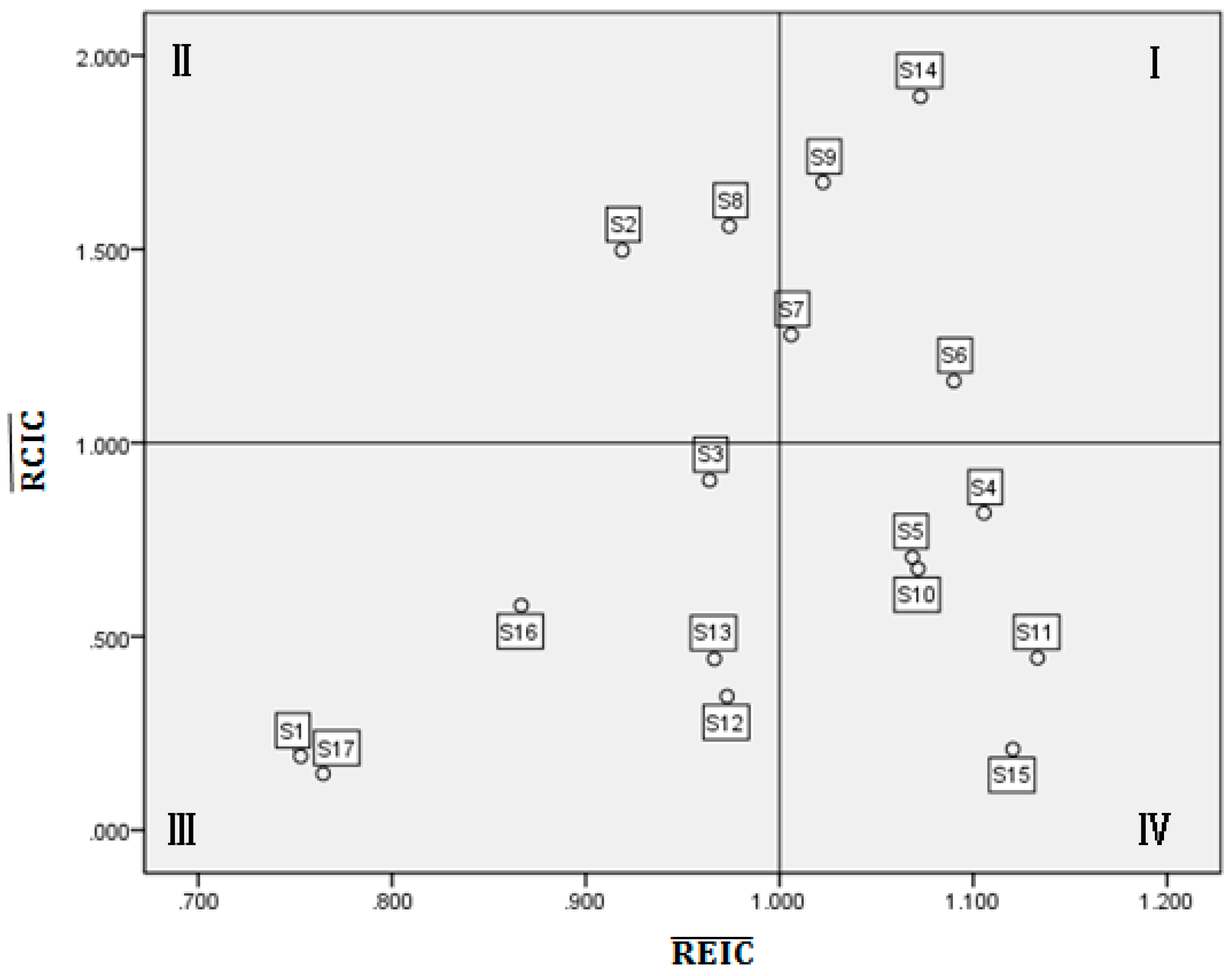
According to Figure 1, there are four HH-type sectors, two LH-type sectors, six LL-type sectors and five HL-type sectors. The average values of $\overline{REIC}$ and $\overline{RCIC}$ in these 17 sectors are 0.992 and 0.854. Generally, most sectors (11 out of 17) are in Quadrants III and IV, which indicates that the development of most sectors in China leads to relatively lower CO₂ emissions in 2010. This affirms that CO₂ emission reduction policies have functioned in most sectors. Regarding the effect of sectoral development on economic growth, about half of the 17 sectors have a relatively strong impact on the macro economy, while the other sectors play a relatively weak role in national economic growth. The top 3 $\overline{REIC}$ sectors are the transportation equipment manufacturing sector (S11), the construction sector (S15) and the textile and related products manufacturing sector (S4), with $\overline{REIC}$s of 1.133, 1.120 and 1.106, respectively. This means that if the value-added of these three sectors were to increase by 1 unit, China’s total GDP would increase by 1.133, 1.120 and 1.106 units, respectively. The top 3 $\overline{RCIC}$s sectors are the electricity, heat, gas and water production and supply sector (S14), the metal smelting and products manufacturing sector (S9) and the non-metallic mineral products manufacturing sector (S8), with $\overline{RCIC}$s of 1.894, 1.673 and 1.559, respectively. If the value-added were to increase by 1 unit in these three sectors, total CO₂ emissions in China would increase by 1.894, 1.673 and 1.559 units, respectively.

Quadrant I in Figure 1 shows the HH-type sectors, which include the electricity, heat, gas and water production and supply sector (S14), the metal smelting and products manufacturing sector (S9), the chemical industry sector (S7) and the papermaking and educational products manufacturing sector (S6). They have large positive effects on promoting national economic growth while also significantly reducing total CO₂ emissions. The $\overline{REIC}$s of these sectors are 1.073 for S14, 1.022 for S9, 1.006 for S7 and 1.090 for S6, which are all higher than 1.000. This means that the effects of sectoral growth in these sectors on the national economy are stronger than the average level of the effects caused by all sectors. Due to a strong nexus with other sectors, the HH-type sectors are the key contributors to China’s economic growth. However, accompanied by strong effects on national economic growth, their CO₂ emissions also contribute to the increase in China’s total CO₂ emissions. The $\overline{RCIC}$s are 1.894 for S14, 1.673 for S9, 1.279 for S7, and 1.159 for S6. Particularly, S14 and S9 have the highest $\overline{RCIC}$s among all the sectors. A high $\overline{RCIC}$ in these sectors is related to high direct fossil energy consumption as well as high indirect consumption from other sectors with which they share a nexus. For example, coal consumption in 2010 for S14 was 1525.72 million tons, accounting for 48.86% of total national coal consumption; S7 not only has high coal consumption (15% of the national total) but also strongly influences the consumption of petroleum products and electricity [59,60].

Quadrant II in Figure 1 shows the LH-type sectors, including the non-metallic mineral products manufacturing sector (S8) and the mining sector (S2). Similar to the HH-type sectors, S8 and S2 also have high $\overline{RCIC}$s, with values of 1.559 and 1.497, respectively, due to their high consumption of fossil energy and a strong nexus with fossil energy-intensive sectors such as the electricity, heat, gas and water production and supply sector (S14). However, the $\overline{REIC}$s of S8 and S2 are lower than 1.000, at only 0.974 and 0.919, respectively. Because of their small effect on national economic growth but large effect on national CO₂ emissions, the LH-type sectors’ development can be considered restrictive.

Compared to the HH-type sectors, the LL-type sectors in Quadrant III in Figure 1 have low $\overline{REIC}$s and $\overline{RCIC}$s. The LL-type sectors include the following sectors: the food and tobacco processing sector (S3), the commercial and transport service sector (S16), the other manufacturing sector (S13), the electric and electronic equipment manufacturing sector (S12), the agriculture sector (S1), and the other services sector (S17). Given their current energy saving and emissions reduction goals, these sectors can be encouraged to a certain extent. The low $\overline{REIC}$ in these sectors is due to their weak nexus with other sectors in China. For example, S1 is an upstream sector that promotes some sectors’ development well but has little effect on other sectors’ growth. Furthermore, S3 is strongly linked to S1 with a weak $\overline{REIC}$, which leads to the low $\overline{REIC}$ in S3. The low $\overline{REIC}$ in S12 is mostly due to the fragmented industry chain. For instance, although China is rich in rare earths, which are important inputs for electric and electronic products, a large portion of products using processed rare earths are imported from foreign countries such as Japan [62]. Therefore, S12 has a weak nexus with the domestic raw material sectors but strongly depends on foreign imports.

The HL-type sectors in Quadrant IV in Figure 1 are most worthy of attention. These sectors have strong positive influences on the whole economy while also maintaining low CO₂ emissions; they include the textile and related products manufacturing sector (S4), the timber processing and furniture manufacturing sector (S5), the machinery industry sector (S10), the transportation equipment manufacturing sector (S11), and the construction sector (S15). 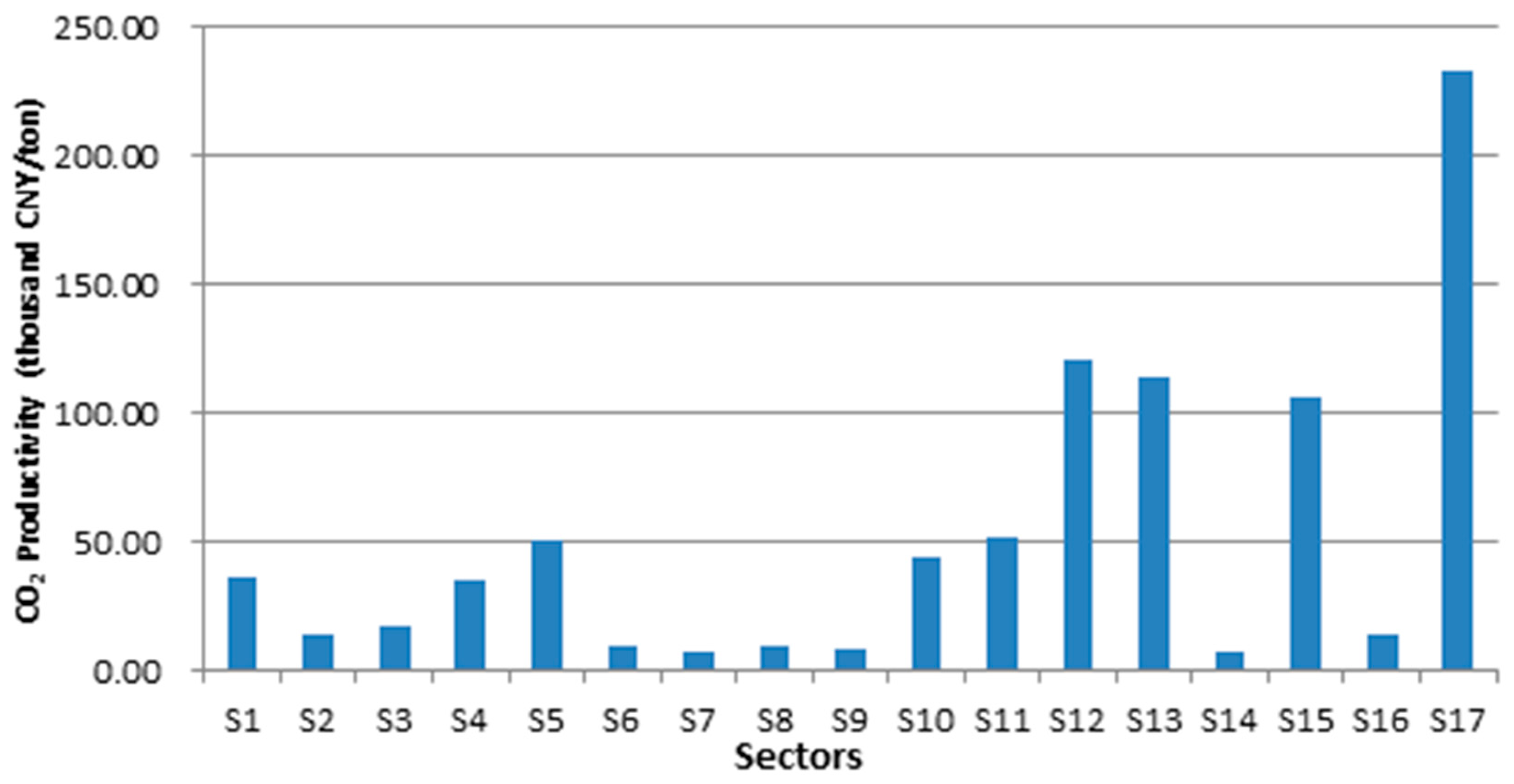Especially, S11, S15 and S4 rank as the top 3 among all sectors in the $\overline{REIC}$, while they have low $\overline{RCIC}$s of 0.445, 0.209 and 0.819, respectively. These sectors are consistent with China’s development expectations for the near future, namely promoting economic development with low emissions. It is slightly surprising that the construction sector (S15) is a HL-type sector because most studies have indicated that it is a carbon-intensive sector [63]. This is because the estimate of $\overline{RCIC}$ for the whole economy is based on the inverse matrix of the matrix of CO₂ productivity. Therefore, if a sector has higher CO₂ productivity compared to the average CO₂ productivity of all sectors, this sector would have a lower $\overline{RCIC}$. The CO₂ productivity of the construction sector (S15) was 106.36 thousand CNY per ton at the current price in 2010, while the average carbon productivity was 51.63 thousand CNY per ton at the current price in 2010. Therefore, China’s construction sector (S15) has the low $\overline{RCIC}$ of 0.209. However, the $\overline{REIC}$ and $\overline{RCIC}$ here only provide an average for the sectors. Each sector in different areas performs differently in both $\overline{REIC}$ and $\overline{RCIC}$; this is analyzed in Section 3.2.

3.2. Regional Analysis

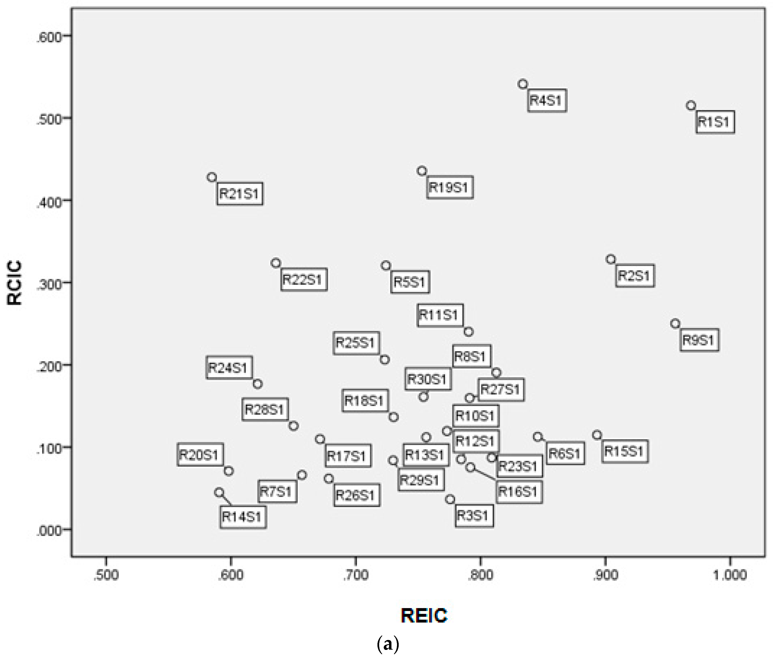
Similar to sectoral performance, most regions (22 regions) in China also have low $\overline{RCIC}$, according to Figure 2. There is one HH-type region, seven LH-type regions, eleven LL-type regions and eleven HL-type regions. The average values of $\overline{REIC}$ and $\overline{RCIC}$ in these 30 regions are 1.000 and 0.833. The top 3 regions in terms of $\overline{REIC}$ are Shandong (R15), at 1.188; Beijing (R1), at 1.123; and Zhejiang (R11), at 1.110. The top 3 regions in terms of $\overline{RCIC}$ are Guizhou (R24), Yunnan (R25) and Jilin (R7). The $\overline{RCIC}$s of these three regions are 1.154, 1.337 and 1.348, respectively.

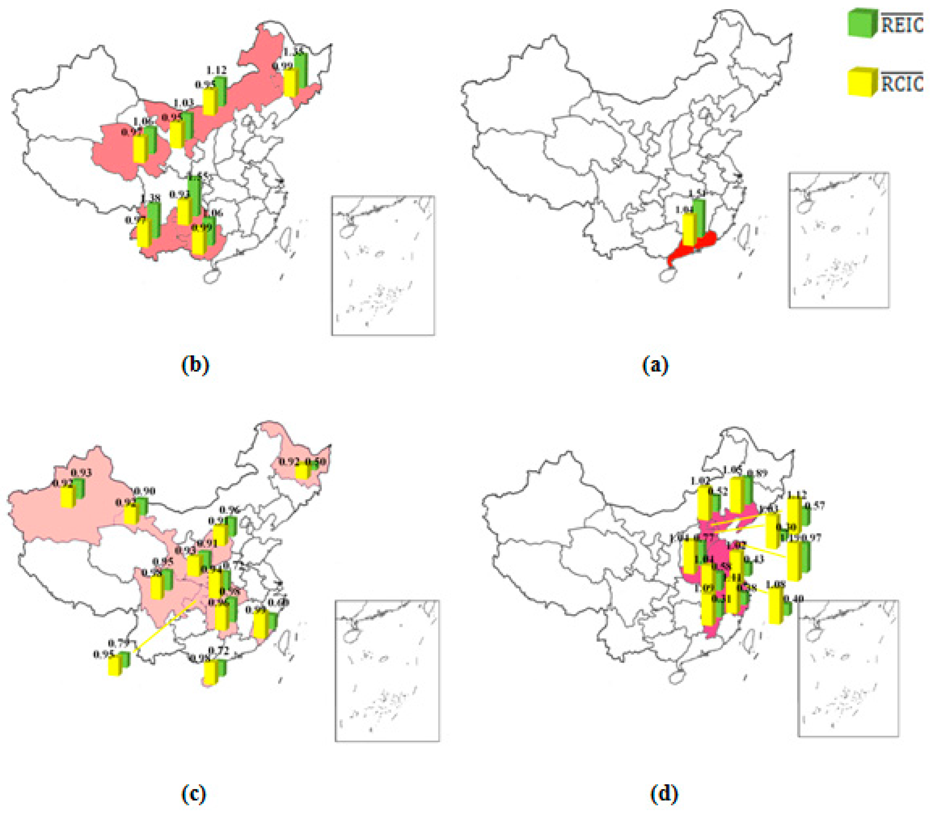
Within the HH-type region, only Guangdong (R19) has high $\overline{REIC}$ and $\overline{RCIC}$ simultaneously, as shown in Figure 2a; the $\overline{REIC}$ and $\overline{RCIC}$ equal 1.043 and 1.312, respectively Guangdong (R19) plays a very important role in supporting the national economy; however, this entails a huge amount of CO₂ emissions. As shown in the map (a) in Figure 2, Guangdong (R19) is located in the southern coastal area that was one of the first regions to open up in China. Due to its proximity to the special administrative regions of Hong Kong and Macao, Guangdong (R19) has a high level of openness [64]. The development of the goods trade and the export-oriented processing industry has promoted economic growth in Guangdong. In 2010, Guangdong’s (R19) GDP reached 4.6 billion Yuan at the current price, accounting for 11% of the national total [64]. At the sectoral level, there are 12 sectors (S3, S4, S5, S6, S7, S8, S9, S10, S11, S13, S14, S15) out of the total of 17 sectors with high $\overline{REIC}$s above 1.000. At the same time, regarding the effect on CO₂ emissions, 7 sectors (S3, S5, S8, S9, S10, S13, S14) in Guangdong (R19) have high $\overline{RCIC}$s above 1.000. This means that 40% of the 17 sectors in Guangdong (R19) are HH-type sectors, which makes Guangdong an HH-type region.

Figure 2b shows the LH-type regions, including Guizhou (R24), Yunan (R25), Jilin (R7), Inner Mongolia (R5), Guangxi (R20), Qinghai (R28) and Ningxia (R29). In these regions, the $\overline{REIC}$ is lower than 1, while the $\overline{RCIC}$ is higher than 1. These regions have different locations, as shown in map (b) in Figure 2: Guangxi (R20) is located in the south, Guizhou (R24) and Yunnan (R25) are located in the southwest, Qinghai (R28) and Ningxia (R29) are located in the northwest, Inner Mongolia (R5) is located in the north, and Jilin (R7) is located in the northeast. However, they all share strong industry and weak service. The $\overline{REIC}s$ of the other services sectors (S17) in these regions are in the range of 0.594 to 0.772. However, the $\overline{REIC}$s of most industry sectors in these regions are approximately 1.000. Most of these regions have rich mineral resources, and mining and mineral products processing are their key sectors. According to sectoral analysis, the mining sector (S2) is a LH-type sector. This may be one of the main reasons that these regions belong to the LH-type.

Figure 2c represents the LL-type regions, which include Hunan (R18), Shanxi (R4), Sichuan (R23), Xinjiang (R30), Shaanxi (R26), Gansu (R27), Chongqing (R22), Hubei (R17), Hainan (R21), Fujian (R13), and Heilongjiang (R8). For the LL-type regions, both the $\overline{REIC}$ and the $\overline{RCIC}$ are lower than 1. Similar to the LH-type regions, most of the LL-type regions are located in the inland area, where it is difficult to attract capital such as foreign direct investment (FDI) and excellent human resources. In these regions, the light industry sectors have had a relatively better economic effect.

The HL-type regions are shown in Figure 2d; they include Shandong (R15), Liaoning (R6), Henan (R16), Anhui (R12), Beijing (R1), Hebei (R3), Jiangsu (R10), Shanghai (R9), Zhejiang (R11), Tianjin (R2), and Jiangxi (R14). Most of these regions are located in eastern coastal China, as shown in map (d) in Figure 2. They have superior trading ports, benefit from many policies supporting economic development, and attract a large amount of capital and talent. In these regions, the industrial structure is reasonable and has a balance of industry and service sectors. Moreover, the $\overline{REIC}$s in most sectors in the HL-type regions are higher than 1. Therefore, these regions promote national economic development significantly. Due to the concentration of capital and talent, production technology has improved rapidly, which not only boosts production efficiency but also improves CO₂ productivity. For example, although Zhejiang (R11) ranks third in $\overline{REIC}$, its $\overline{RCIC}$ was only 0.380.

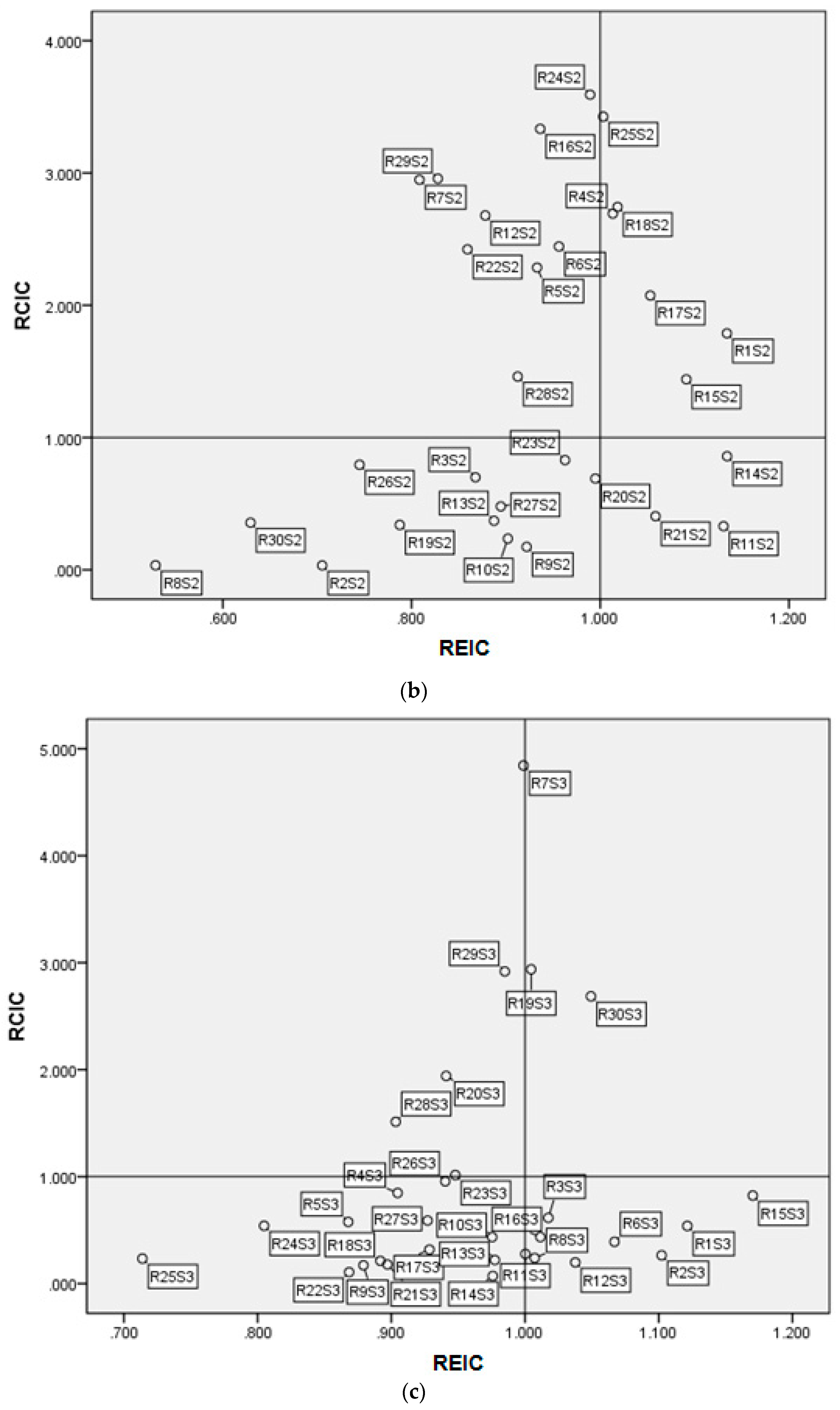
3.3. Sectoral-Regional Integrated Economy-Carbon Nexus Analysis

To determine the regular distribution of economic sectors, we observed the economy-carbon nexus from both regional and sectoral perspectives (shown in Appendix Figure A3a–q).

For the agriculture sector (S1) and the other services sector (S17), the S1 and S17 in all regions are scattered in the LL-type (Quadrant III). This means that the S1 and S17 in all regions exhibit low economic influence and low CO₂ emissions influence on other sectors. Therefore, S1 and S17 in all regions should focus on improving their economic influence to transition to the HL-type.

For the mining sector (S2), 21 regions out of 30 regions are scattered in the LH-type (Quadrant II) and the LL-type (Quadrant III). This means that S2 in most regions shows low economic influence. However, the influences of CO₂ emissions are different in these 21 regions due to their different energy structures. In addition, the other 3 regions, which include Zhejiang (R11), Jiangxi (R14) and Hainan (R21), belong to the HL-type. Therefore, the energy consumption structures, production technology and industrial chain constructions in these 3 regions can be used as benchmarks for other regions.

For the food and tobacco processing sector (S3), the transportation equipment manufacturing sector (S12) and the electrical and electronic equipment manufacturing sector (S13), most regions are concentrated in the LL-type (Quadrant III) and the HL-type (Quadrant IV). This means that when promoting economic development, S3, S12 and S13 in most regions of China have relatively low CO₂ emissions influences. However, their levels of economic influence are different because production technology and industrial structures are different in these regions. Moreover, S3 in 8 regions, S12 in 8 regions and S13 in 12 regions belong to the HL-type, and these regions can be used as benchmarks for other regions.

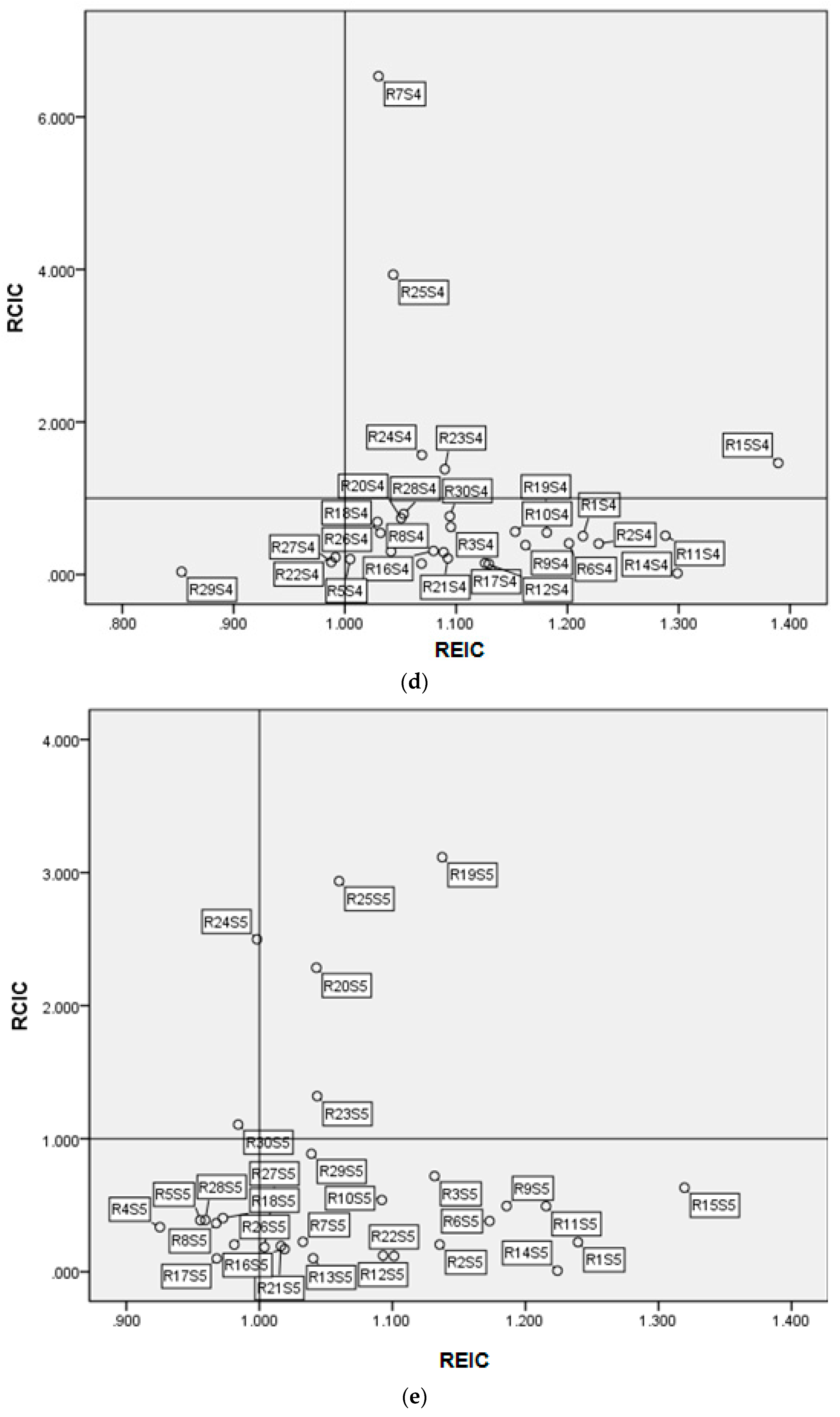
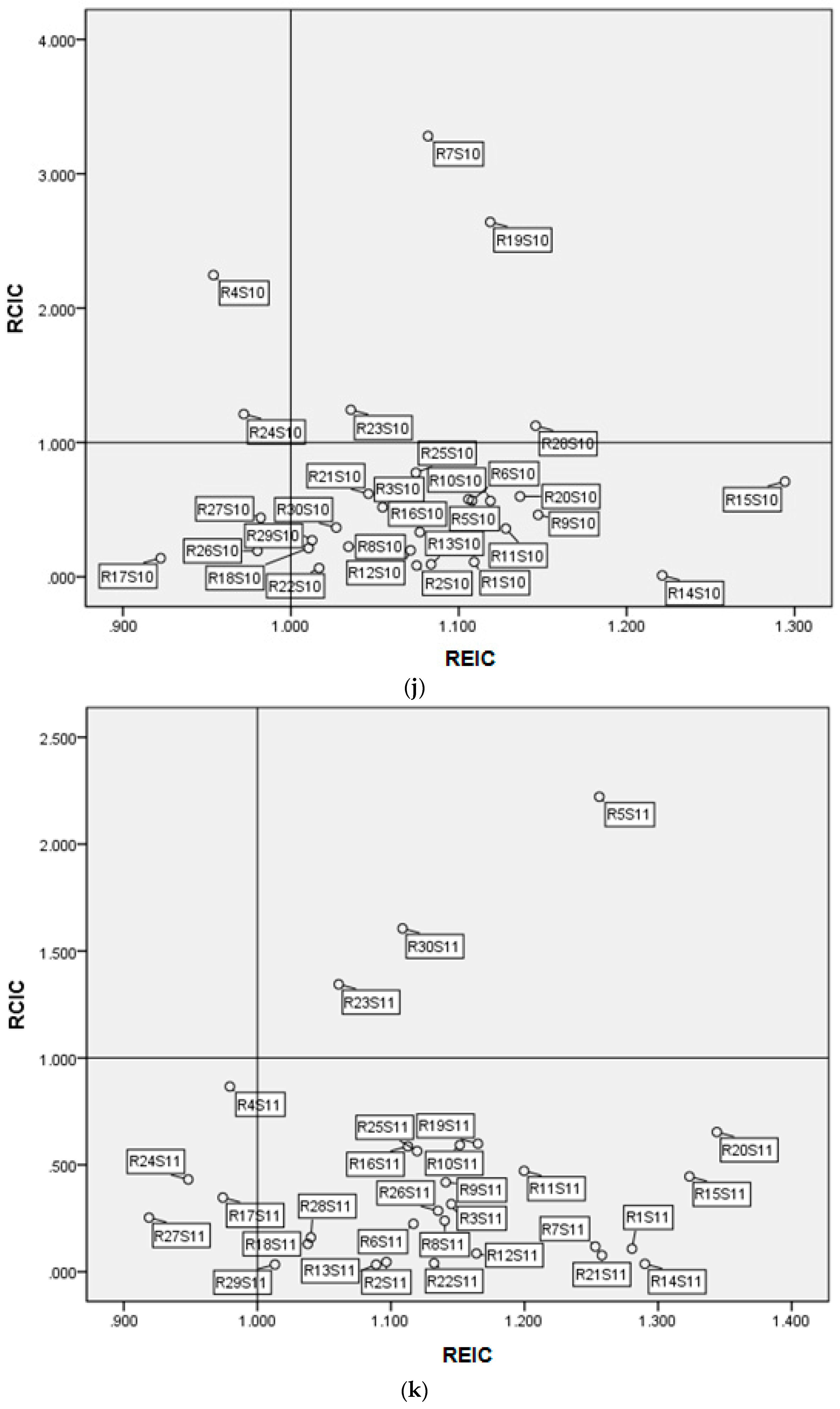
For the textile and related products manufacturing sector (S4), the mechanical industry sector (S10) and the transportation equipment manufacturing sector (S11), most regions are concentrated in the HL-type (Quadrant IV). For the above three sectors, S4 in 22 regions, S10 in 21 regions and S11 in 23 regions belong to the HL-type. Generally, the development of S4, S10 and S11 in China show high economic influence and low CO₂ emissions influence, though there are some regions scattered in the LL-type, HH-type or LH-type. Therefore, S4, S10 and S11 can be considered the priority sectors that that should be supported to promote China's economic development in the future.

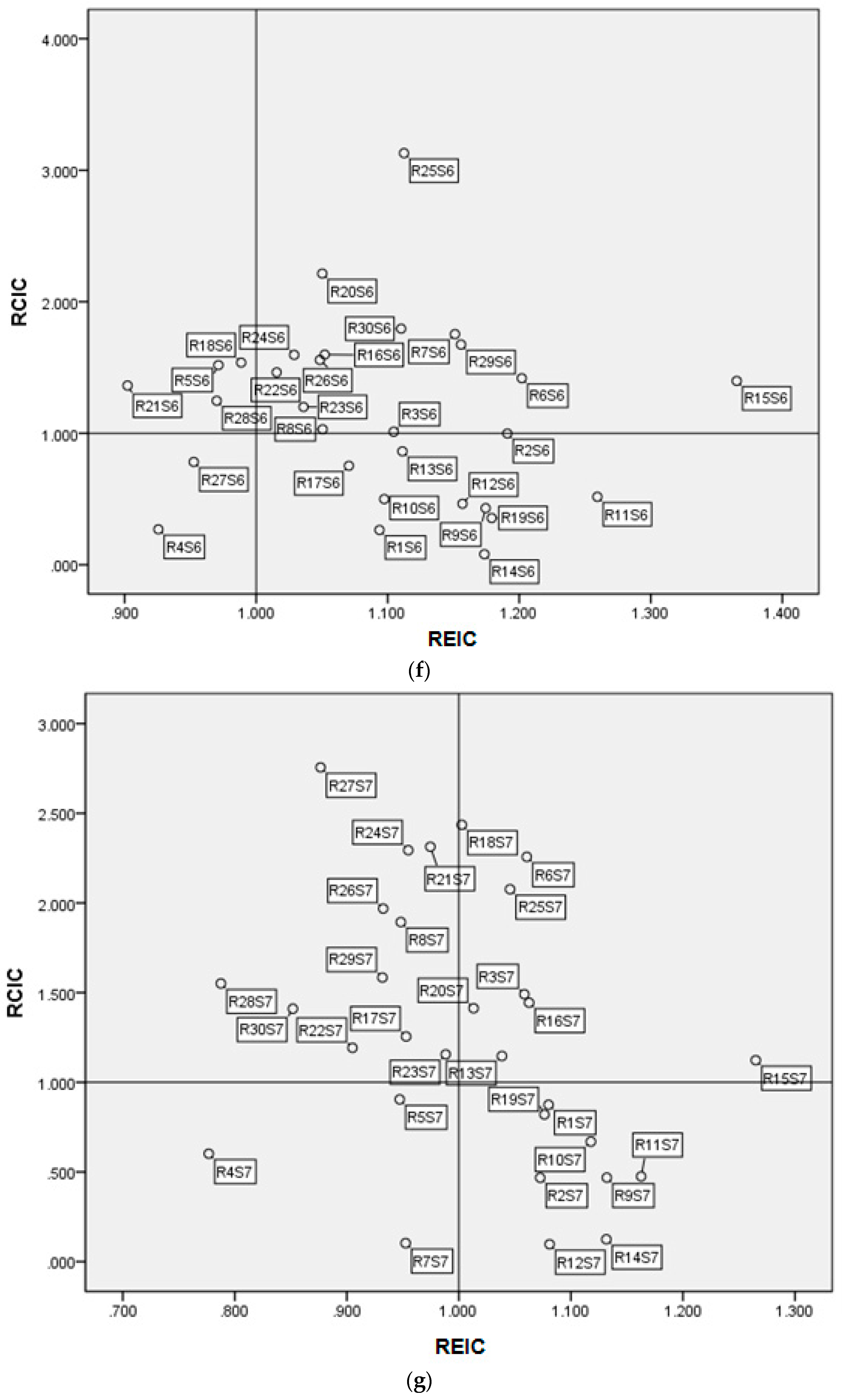
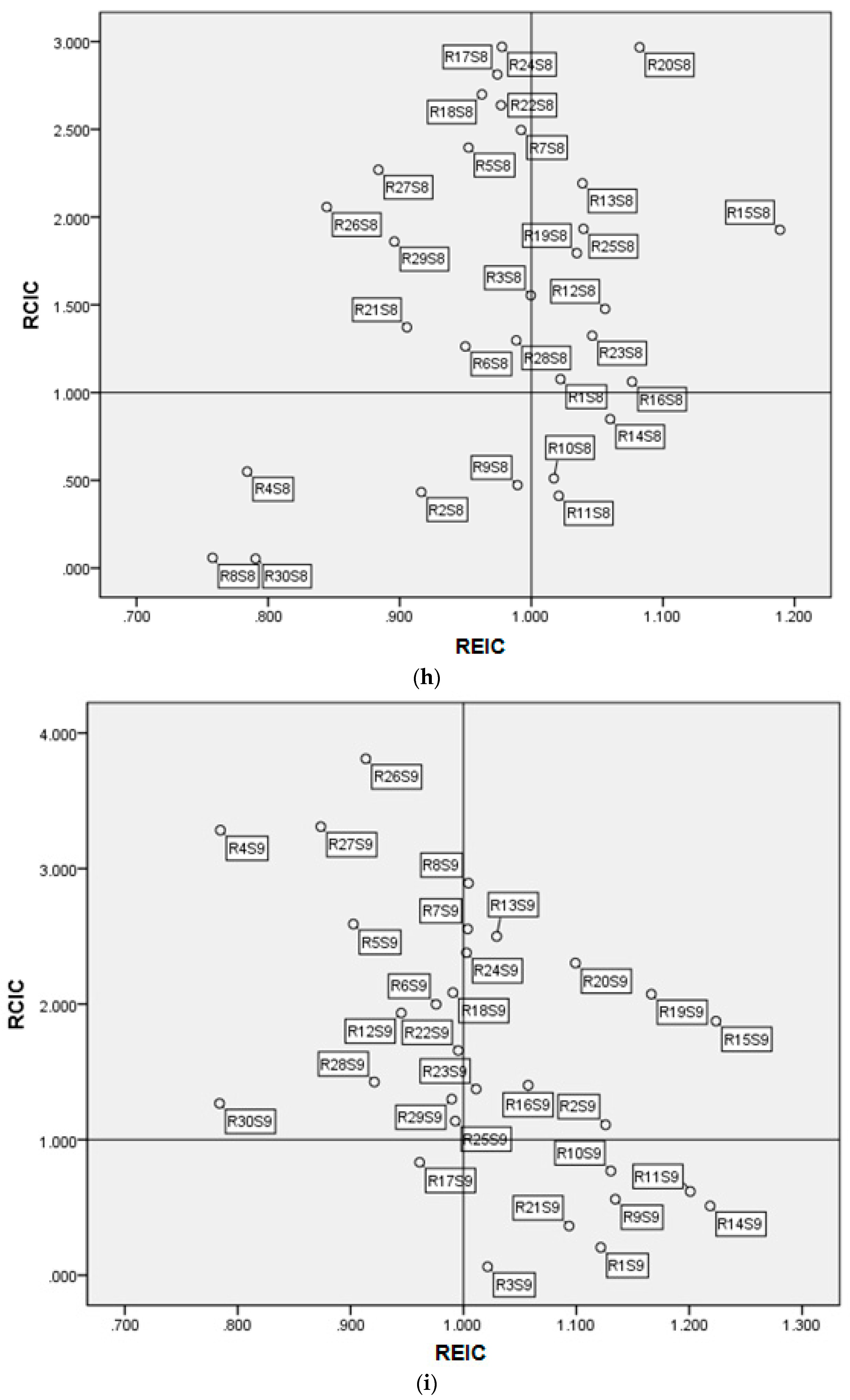
For the papermaking and educational products manufacturing sector (S6), 24 regions are concentrated in the HH-type (Quadrant I) and in the HL-type (Quadrant IV). This indicates that S6hasstrongeconomic influence in most regions. Out of these 24 regions, there are 14 regions and 10 regions distributed in the HH-type and HL-type, respectively. This means that S6 in most regions should focus on reducing its CO₂ emission influences.

For the chemical industry sector (S7), the non-metallic mineral products manufacturing sector (S8), the metal smelting and products manufacturing sector (S9) and the electricity, heat, gas and water production and supply sector (S14), most regions are scattered in the HH-type (Quadrant I) and LH-type (Quadrant II). This illustrates that these 4 sectors in most regions show high CO₂ emissions influence. It is exciting that S7 in 8 regions, S8 in 3 regions, S9 in 7 regions and S14 in 6 regions belong to the HL-type, which can be the benchmark for other regions.

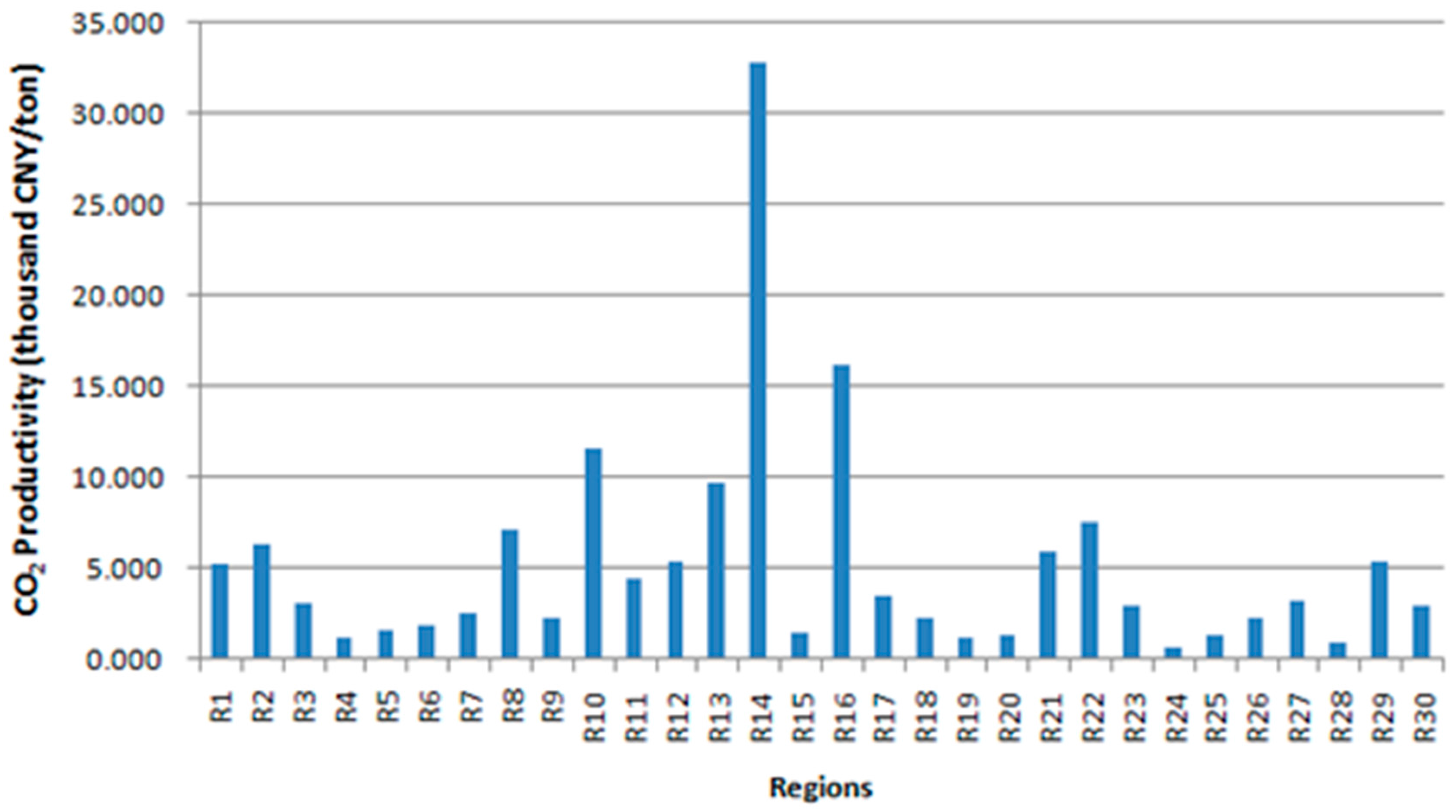
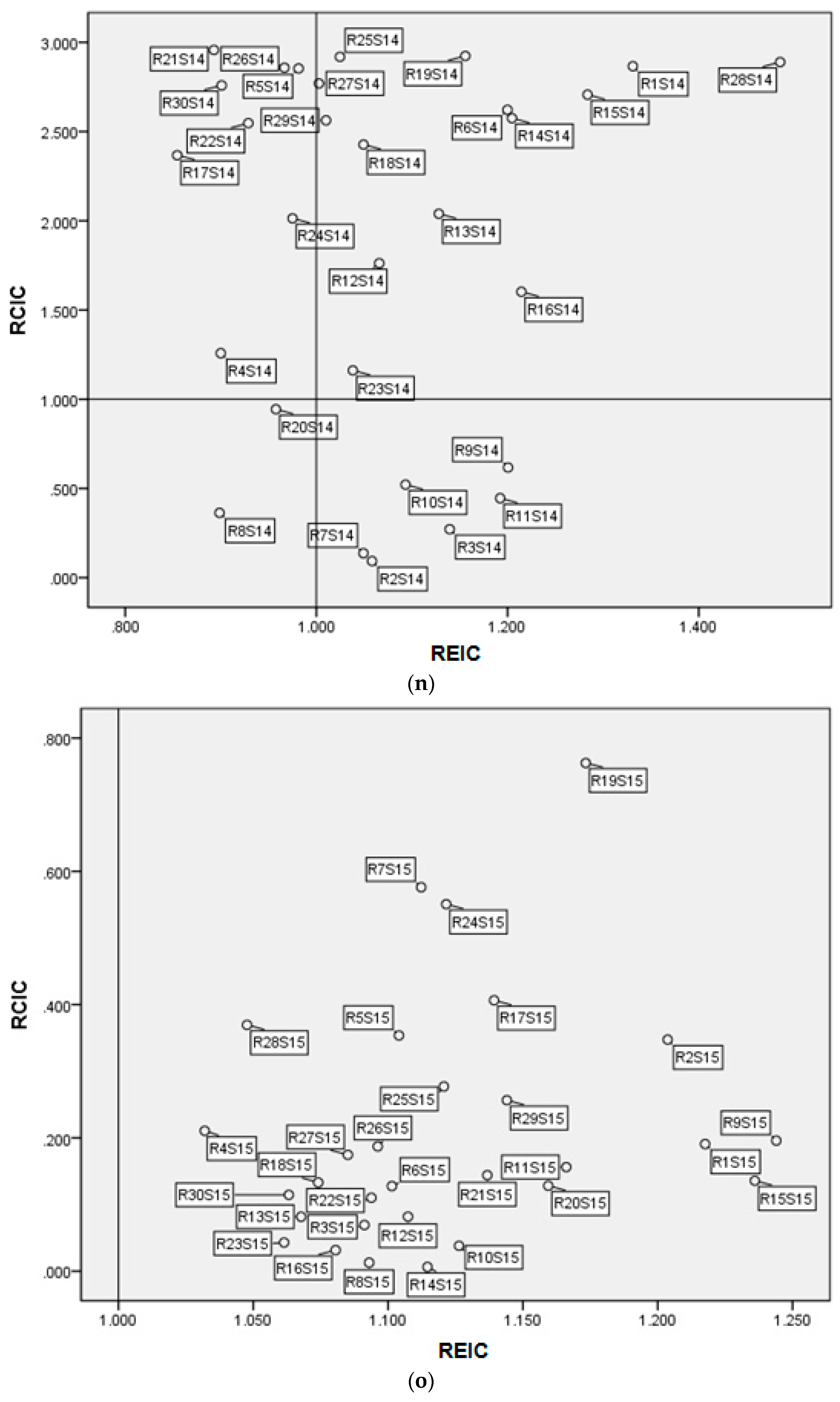
For the construction sector (S15), it is slightly surprising that S15 in all regions is scattered in the HL-type (Quadrant IV). This indicates that S15 has a strong economic influence on both the downstream and upstream sectors. Moreover, in all regions S15 shows low CO₂ emission influences. Similarly, Meng et al. [13] studied China’s CO₂ emissionsin17 sectors in 2002 and 2007 and found that construction accounted for just 0.8% of CO₂ emissions in 2002 (ranking 10th out of all 17 sectors) and 0.6% of CO₂ emissions in 2007 (ranking 12th out of all 17 sectors). This may be because the estimate of RCICs for the whole economy is based on the Leontief inverse coefficient and CO₂ productivity. Therefore, S15 has a lower CO₂ emissions influence due to its larger CO₂ productivity compared to the average of CO₂ productivities for all sectors.

For the commerce and transportation service sector (S16), there are 24 regions scattered in the LL-type (Quadrant III). Moreover, there is no HH-type region in S16. This means that S16 in most regions has low CO₂ emissions influence and low economic influence. It is exciting that in two regions (Beijing (R1) and Shanghai (R9)); S16 belongs to the HL-type and can be the benchmark for other regions.

4. Concluding Remarks

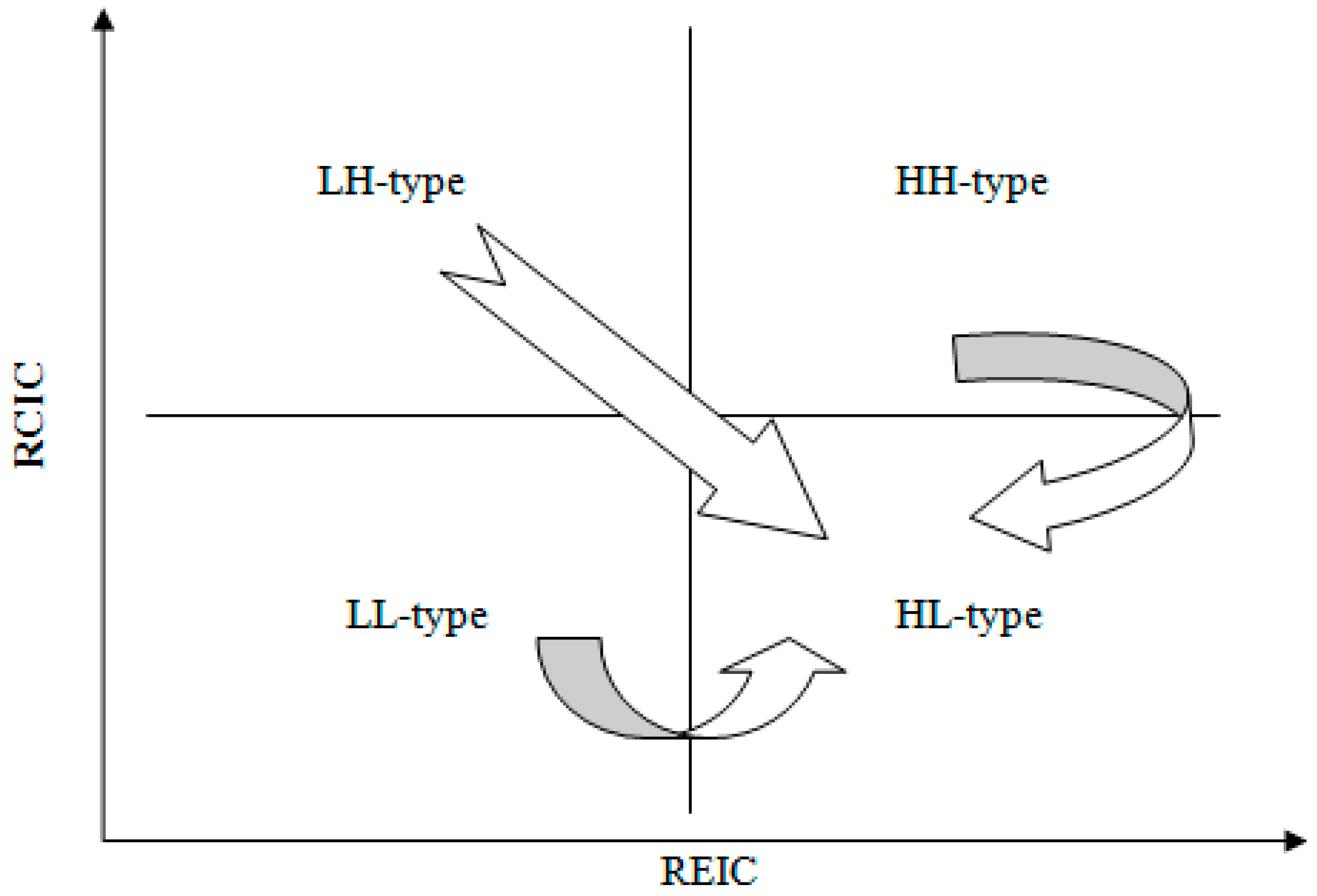
Currently, China faces the dual pressures of economic growth and CO₂ emissions reduction at both the national and local levels. In this study, a MRIO model is used to determine benchmark sectors and notable patterns of regional development for policy-makers. Holistic policy implications are depicted in Figure 3, in which the LH-type, HH-type and LL-type sectors or regions should be transitioned to the HL-type because the HL-type produces a high economic influence coefficient and a low CO₂ emissions influence coefficient, which is the ideal benchmark.

At the sectoral level, specific policy implications mainly focus on promoting economic influence and reducing CO₂ emissions influence.

The HL-type sectors are benchmarking sectors because of their high economic influence and low CO₂ emissions influence; they should maintain their current development and continue to enhance their economic influence while reducing their CO₂ emissions.

For the sectors with low economic influence, more economic policy implications should be considered. For example, the Chinese government can extend and upgrade the industrial chain in the same region and to the other regions and tighten the relationship between upstream and downstream to enhance the sector’s economic influence.

For the sectors with high CO₂ emissions influence, more attention should be focused on how to reduce CO₂ emissions in these sectors’ production activities. Specific policy implications include improving energy efficiencies through improved production technology and adjusting the energy consumption structure, especially by enhancing the proportion of clean energy derived from, e.g., wind power and solar power. Moreover, raising the cost of CO₂ emissions by implementing carbon taxes and carbon emissions trading is also a useful method because it can force the transition of both the energy consumption structure and improvements to energy efficiency.

At the regional level, both geographic location and preferential policies of the past determine, to a large extent, whether a region can become the HL-type.

The HH-type region of Guangdong can exploit the advantages of its geographical location and early opening-up, acquire the advanced production technology of foreign countries, and adjust its energy structure to reduce its CO₂ emissions.

For the inland regions belonging to the LH-type and the LL-type, the most important measures include constructing transportation infrastructure and attracting capital and talent to enhance these regions’ economic influence in the national economy. Moreover, these regions should strengthen communications with the HL-type regions to improve production technology and further reduce their CO₂ emissions. Specifically, the LH-type regions should increase the value-added proportion of HL-type sectors in regional GDP.

References

1. Meng, M.; Niu, X.D.; Gao, Q. Decomposition analysis of Chinese provincial economic growth through carbon productivity analysis: Environmental Progress & Sustainable. Energy 2014, 33, 251–255. [Google Scholar]
2. International Energy Agency (IEA). World Energy Outlook 2007: China and India Insights; IEA: Paris, France, 2007. [Google Scholar]
3. Netherlands Environmental Assessment Agency (MNP). China Now No. 1 in CO2 Emissions. USA in Second Position. MNP: Bilthoven, The Netherlands, 2007. Available online: http://www.pbl.nl/en/dossiers/Climatechange/ (accessed on 20 December 2016).
4. Guan, D.; Peters, G.P.; Weber, C.L.; Hubacek, K. Journey to world top emitter: An analysis of the driving forces of China’s recent CO2 emissions surge. Geophys. Res. Lett. 2009, 36, 1–5. [Google Scholar] [CrossRef]
5. Zhou, N.; Fridley, D.; Mcneil, M.; Zheng, N.; Ke, J.; Levine, M. China’s Energy and Carbon Emissions Outlook to 2050; US Department of Energy, Ernest Orlando Lawrence Berkeley National Laboratory: Berkeley, CA, USA, 2011.
6. Feng, K.; Siu, Y.L.; Guan, D.; Hubacek, K. Analyzing drivers of regional carbon dioxide emissions for China. J. Ind. Ecol. 2012, 16, 600–611. [Google Scholar] [CrossRef]
7. Liu, Z.; Geng, Y.; Lindner, S.; Guan, D. Uncovering China’s greenhouse gas emission from regional and sectoral perspectives. Energy 2012, 45, 1059–1068. [Google Scholar] [CrossRef]
8. EIA. International Energy Outlook 2016 Table: World Carbon Dioxide Emissions by Region. 2016. Available online: http://www.eia.gov/forecasts/aeo/data/browser/ (accessed on 11 October 2016). [Google Scholar]
9. United Nations Framework Convention on Climate Change (UNFCC). Available online: https://unfccc.int/resource/docs/convkp/conveng.pdf (accessed on 20 December 2016).
10. Lin, B.Q.; Ouyang, X.L. Analysis of energy-related CO2 (carbon dioxide) emissions and reduction potential in the Chinese non-metallic mineral products industry. Energy 2014, 68, 688–697. [Google Scholar] [CrossRef]
11. Gregg, J.S.; Andres, R.J.; Marland, G. China: Emissions pattern of the world leader in CO2 emissions from fossil fuel consumption and cement production. Geophys. Res. Lett. 2008, 35. [Google Scholar] [CrossRef]
12. Feng, K.; Davis, S.J.; Sun, L.; Li, X.; Guane, D.; Liuh, W.; Liuf, Z.; Hubacek, K. Outsourcing CO2 within China. PNAS 2013, 110, 11654–11659. [Google Scholar] [CrossRef] [PubMed] [Green Version]
13. Meng, B.; Xue, J.; Feng, K.; Guan, D.; Fu, X. China’s inter-regional spillover of carbon emissions and domestic supply chains. Energy Policy 2013, 61, 1305–1321. [Google Scholar] [CrossRef]
14. Yuan, R.; Zhao, T. A combined input-output and sensitivity analysis of CO2 emissions in the high energy-consuming industries: A case study of China. Atmos. Pollut. Res. 2012, 7, 315–325. [Google Scholar] [CrossRef]
15. Xu, B.; Lin, B.Q. Carbon dioxide emissions reduction in China’s transport sector: A dynamic VAR (vector auto regression) approach. Energy 2015, 83, 486–495. [Google Scholar] [CrossRef]
16. Ebrahim, K.; Atefeh, M.; Somayeh, A. Integrating building and transportation energy use to design a comprehensive greenhouse gas mitigation strategy. Appl. Energy 2016, 165, 234–243. [Google Scholar] [CrossRef]
17. Moreira, J.R.; Pacca, S.A.; Parente, V. The future of oil and bio-ethanol in Brazil. Energy Policy 2014, 65, 7–15. [Google Scholar] [CrossRef]
18. Carlos, E.S.; Márcio, A.D. The role of rail transit systems in reducing energy and carbon dioxide emissions: The case of the city of Rio de Janeiro. Sustainability 2016, 8, 150. [Google Scholar] [CrossRef]
19. Machado, G.; Schaeffer, R.; Worrell, E. Energy and carbon embodied in the international trade of Brazil: An input-output approach. Ecol. Econ. 2015, 39, 409–424. [Google Scholar] [CrossRef]
20. Soytas, U.; Sari, R.; Ewing, B.T. Energy consumption, income, and carbon emissions in the United States. Ecol. Econ. 2007, 62, 482–489. [Google Scholar] [CrossRef]
21. Kundak, M.; Lazic, L.; Crnko, J. CO2 emissions in the steel industry. Metalurgija 2009, 48, 193–197. [Google Scholar]
22. Kyunsuk, C.; Hiroyuki, M.; Hyunjoung, L.; Sohn, I. Achieving a carbon neutral society without industry contraction in the five major steel producing countries. Sustainability 2016, 8, 484. [Google Scholar] [CrossRef]
23. Sauerbeck, D.R. CO2 emissions and C sequestration by agriculture-perspectives and limitations. Nutr. Cycl. Agroecosyst. 2011, 60, 253–266. [Google Scholar] [CrossRef]
24. Clara, I.; Pardo, M.; Semida, S. Analysis of energy use and CO2 emission in service industries: Evidence from Sweden. Renew. Sustain. Energy Rev. 2012, 16, 5285–5294. [Google Scholar]
25. Ge, J.P.; Lei, Y.L. Carbon emissions from the service sector: An input-output application to Beijing, China. Clim. Res. 2014, 60, 13–24. [Google Scholar] [CrossRef]
26. Xue, B.; Geng, Y.; Katrin, M.; Lu, C.P.; Ren, W.X. Understanding the causality between carbon dioxide emission, fossil energy consumption and economic growth in developed countries: An empirical study. Sustainability 2014, 6, 1037–1045. [Google Scholar] [CrossRef]
27. Long, R.Y.; Shao, T.X.; Chen, H. Spatial econometric analysis of China’s province-level industrial carbon productivity and its influencing factors. Appl. Energy 2015, 166, 210–219. [Google Scholar] [CrossRef]
28. Yuan, R.; Zhao, T. Changes in CO2 emissions from China’s energy-intensive industries: A subsystem input-output decomposition analysis. J. Clean. Prod. 2016, 117, 98–109. [Google Scholar] [CrossRef]
29. Ashfaq, A.; Zhao, Y.H.; Muhammad, S.; Sadia, B.; Zhang, Z.H.; Wang, S.; Liu, Y. Carbon emissions, energy consumption and economic growth: An aggregate and disaggregate analysis of the Indian economy. Energy Policy 2016, 96, 131–143. [Google Scholar]
30. Sahu, S.K.; Narayanan, K. Energy Use Patterns and Firm Performance: Evidence from Indian Industries. J. Energy Dev. 2014, 40, 111–133. [Google Scholar]
31. Carbon Dioxide Information Analysis Center (CDIA). Available online: http://cdiac.ornl.gov/ (accessed on 20 December 2016).
32. Singh, S.K. Future mobility in India: Implications for energy demand and CO2 emission. Transp. Policy 2006, 13, 398–412. [Google Scholar] [CrossRef]
33. Shao, L.; Guan, D.B.; Zhang, N.; Shan, Y.L.; Che, G.Q. Carbon emissions from fossil fuel consumption of Beijing in 2012. Environ. Res. Lett. 2016, 11, 114028. [Google Scholar] [CrossRef]
34. Zhu, Q.; Peng, X.Z.; Wu, K.Y. Calculation and decomposition of indirect carbon emissions from residential consumption in China based on the input-output model. Energy Policy 2012, 48, 618–626. [Google Scholar] [CrossRef]
35. Ge, J.P.; Lei, Y.L.; Yu, C. Multiscale input-output subsystem model of methane and nitrous oxide emissions from the service sector: A case study of Beijing, China. Clim. Res. 2016, 69, 247–259. [Google Scholar] [CrossRef]
36. Moses, L.N. The stability of interregional trading patterns and input-output analysis. Am. Econ. Rev. 1955, 45, 803–832. [Google Scholar]
37. Isard, W. Interregional and regional input–output analysis: A model of a space economy. Rev. Econ. Stat. 1951, 33, 318–328. [Google Scholar] [CrossRef]
38. Chenery, H.B. Pattens of industrial growth. Am. Econ. Rev. 1960, 50, 624–654. [Google Scholar]
39. Chenery, H.B.; Watanabe, T. The pattern of Japanese growth, 1914–1954. Eeonometrica 1962, 30, 98–139. [Google Scholar] [CrossRef]
40. Leontief, W. Environmental repercussions and the economic structure: An input–output approach. Rev. Econ. Stat. 1970, 52, 262–271. [Google Scholar] [CrossRef]
41. Leontief, W.; Strout, A. Chapter: Structural interdependence and economic development. In Multi-Regional Input–Output Analysis; Palgrave Macmillan Press: London, UK, 1963; pp. 119–150. [Google Scholar]
42. Zhang, W.Q.; Peng, S.J.; Sun, C.W. CO2 emissions in the global supply chains of services: An analysis based on a multi-regional input–output model. Energy Policy 2015, 86, 93–103. [Google Scholar] [CrossRef]
43. Minx, J.C.; Baiocchi, G.; Peters, G.P.; Weber, C.L.; Guan, D.; Hubacek, K. A carbonizing dragon: China’s fast growing CO2 emissions revisited. Environ. Sci. Technol. 2011, 45, 9144–9153. [Google Scholar] [CrossRef]
44. Liu, W.; Chen, J.; Tang, Z.; Liu, H.; Han, D.; Li, F. Theories and Practice of Constructing China’s Inter Regional Input–Output Tables between 30 Provinces in 2007; China Statistics Press: Beijing, China, 2012.
45. Wang, Y.; Wang, W.; Mao, G.; Cai, H.; Zuo, J.; Wang, L.; Zhao, P. Industrial CO2 emissions in China based on the hypothetical extraction method: Nexus analysis. Energy Policy 2013, 62, 1238–1244. [Google Scholar] [CrossRef]
46. Chen, G.W.; Michalis, H.; Thomas, W. Urban carbon transformations: Unraveling spatial and inter-sectoral nexus for key city industries based on multi-region input-output analysis. J. Clean. Prod. 2016, 4, 1–17. [Google Scholar] [CrossRef]
47. Li, J.S.; Chen, B.; Chen, G.Q.; Wei, W.D.; Wang, X.B.; Ge, J.P.; Dong, K.Q.; Xia, H.H.; Xia, X.H. Tracking mercury emission flows in the global supply chains: A multi-regional input-output analysis. J. Clean. Prod. 2017, 140, 1470–1492. [Google Scholar] [CrossRef]
48. Su, B.; Ang, B.W. Multi-region input–output analysis of CO2 emissions embodied in trade: The feedback effects. Ecol. Econ. 2011, 71, 42–53. [Google Scholar] [CrossRef]
49. Su, B.; Ang, B.W. Input-output analysis of CO2 emissions embodied in trade: A multi-region model for China. Appl. Energy 2014, 114, 377–384. [Google Scholar] [CrossRef]
50. Zhang, Z.; Guo, J.E.; Hewings, G.J. The effects of direct trade within China on regional and national CO2 emissions. Energy Econ. 2014, 46, 161–175. [Google Scholar] [CrossRef]
51. Zhang, Y.; Tang, Z. Driving forces of carbon embodied in China’s provincial exports. Energy Econ. 2015, 51, 445–454. [Google Scholar] [CrossRef]
52. Su, B.; Thomson, E. China’s carbon emissions embodied in (normal and processing) exports and their driving forces, 2006–2012. Energy Econ. 2016, 59, 414–422. [Google Scholar] [CrossRef]
53. Su, B.; Ang, B.W. Input-output analysis of CO2 emissions embodied in trade: Competitive versus non-competitive imports. Energy Policy 2013, 56, 83–87. [Google Scholar] [CrossRef]
54. Leontief, W. Quantitative Input and Output Relations in the Economic Systems of the United States. Rev. Econ. Stat. 1936, 18, 105–125. [Google Scholar] [CrossRef]
55. Su, B.; Ang, B.W. Input-output analysis of CO2 emissions embodied in trade: The effects of spatial aggregation. Ecol. Econ. 2010, 70, 10–18. [Google Scholar] [CrossRef]
56. Su, B.; Huang, H.C.; Ang, B.W.; Zhou, P. Input-output analysis of CO2 emissions embodied in trade: The effects of sector aggregation. Energy Econ. 2010, 32, 166–175. [Google Scholar] [CrossRef]
57. Liu, W.D.; Tang, Z.P.; Chen, J. China’s 30 Provinces Regional Input-Output Table in 2010; China Statistics Press: Beijing, China, 2014. (In Chinese)
58. National Bureau of Statistics (NBS). China Statistical Yearbook, 2011; China Statistics Press: Beijing, China, 2011.
59. National Bureau of Statistics (NBS). China Energy Statistical Yearbook, 2011; China Statistics Press: Beijing, China, 2011.
60. National Bureau of Statistics (NBS). China Energy Statistical Yearbook, 2012; China Statistics Press: Beijing, China, 2012.
61. Parry, M.L.; Canziani, O.F.; Palutikof, J.P.; van der Linden, P.J.; Hanson, C.E. Climate Change 2007—Mitigation of Climate Change (IPPC WGIII AR4); Cambridge University Press: Cambridge, UK, 2007. [Google Scholar]
62. Ge, J.P.; Lei, Y.L.; Zhao, L.R. China’s rare earth supply forecast in 2015: A dynamic computable general equilibrium analysis. Minerals 2016, 6, 95. [Google Scholar] [CrossRef]
63. Hong, J.K.; Shen, G.Q.; Guo, S.; Xue, F.; Zheng, W. Energy use embodied in China’s construction industry: A multi-regional input–output analysis. Renew. Sustain. Energy Rev. 2016, 53, 1303–1312. [Google Scholar] [CrossRef]
64. Wang, P.; Zhu, B.Z. Estimating the contribution of industry structure adjustment to the carbon intensity target: A case of Guangdong. Sustainability 2016, 8, 355. [Google Scholar] [CrossRef]
Figure 1. Matrix of the R E I C ¯ and R C I C ¯ of China’s 17 sectors in 2010.
Energies 10 00093 g001
Figure 2. Map of different types of regions in China in 2010. (a) HH-type regions; (b) LH-type regions; (c) LL-type regions; (d) HL-type regions
Energies 10 00093 g002
Figure 3. Policy implications for different types of sectors or regions.
Energies 10 00093 g003