
Performance Evaluation of a Solar-Powered Regenerative Organic Rankine Cycle in Different Climate Conditions

Abstract
:1. Introduction
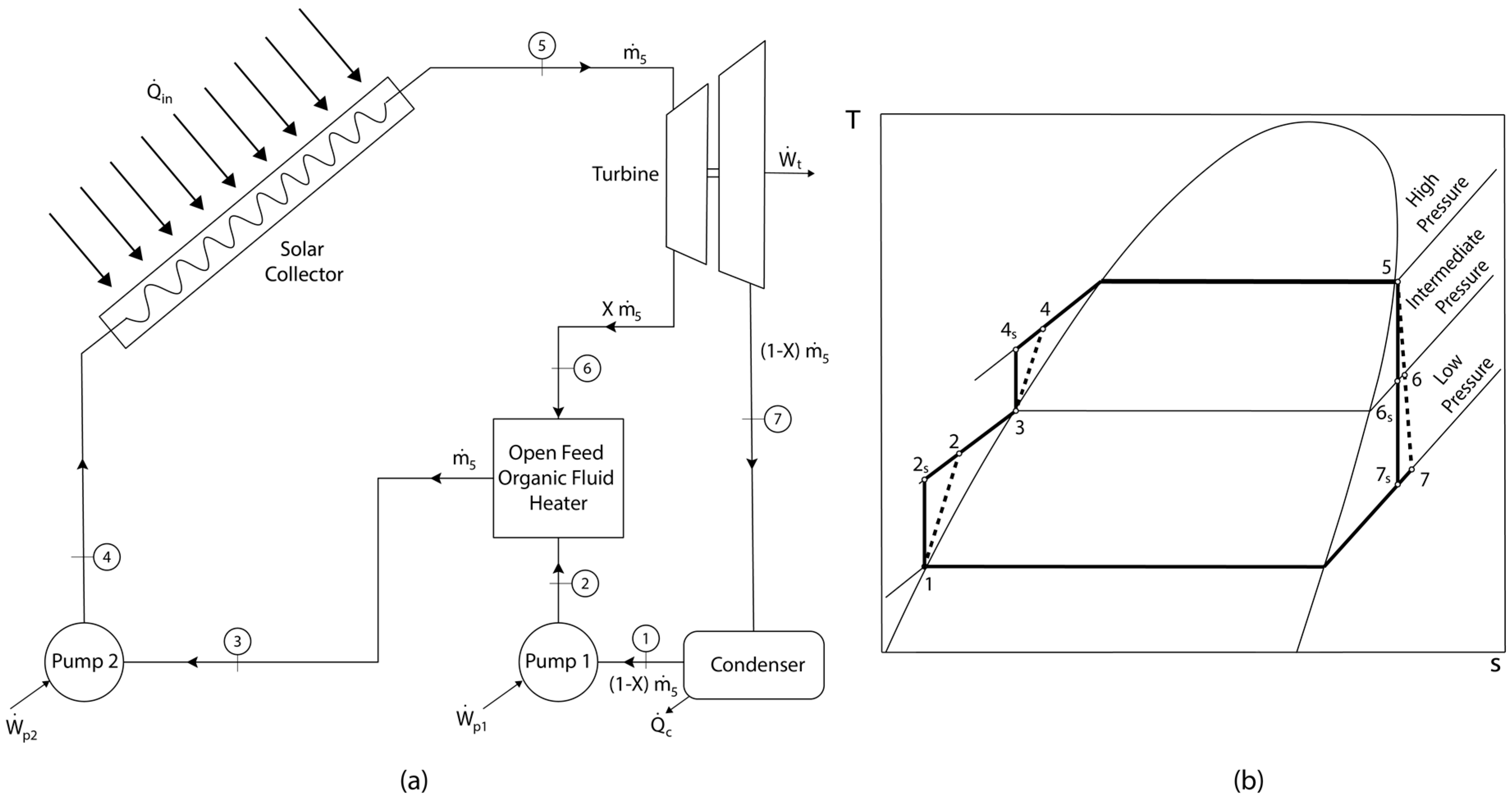
2. System Model
- a.
- Pump 1 (Process 1–2): The pump power can be determined as:where is the ideal power of Pump 1, is the isentropic efficiency of Pump 1, is the mass flow rate of the working fluid at State 5, is the fraction of the extracted fluid from the first stage of the turbine, and , , and are the enthalpy values of the working fluid at the pump inlet, the ideal enthalpy value at the pump exit, and the actual value at the pump exit, respectively.The exergy destruction rate for Pump 1 is:where is the pump exergy rate and and are the exergy rates for State 2 and State 1, respectively.The exergy rate of Pump 1 is given by:The exergy rate change from State 1 to State 2 can be estimated as:where , , and are the temperature at the dead state (298 K), and entropy values of the working fluid for States 1 and 2, respectively.
- b.
- Pump 2 (Process 3–4): The power required for Pump 2 is given bywhere is the ideal power of Pump 2, is the isentropic efficiency of Pump 2, and and are the enthalpy values of the working fluid at State 3 and 4, which are the inlet and outlet of Pump 2, respectively.The exergy destruction rate for Pump 2 can be determined as:where is the exergy rate of Pump 2 and and are the exergy rates for State 4 and State 3, respectively.The exergy rate of Pump 2 is given by:The change in exergy rate between States 4 and 3 is:where and are the entropy values of the working fluid at States 4 and 3, respectively.
- c.
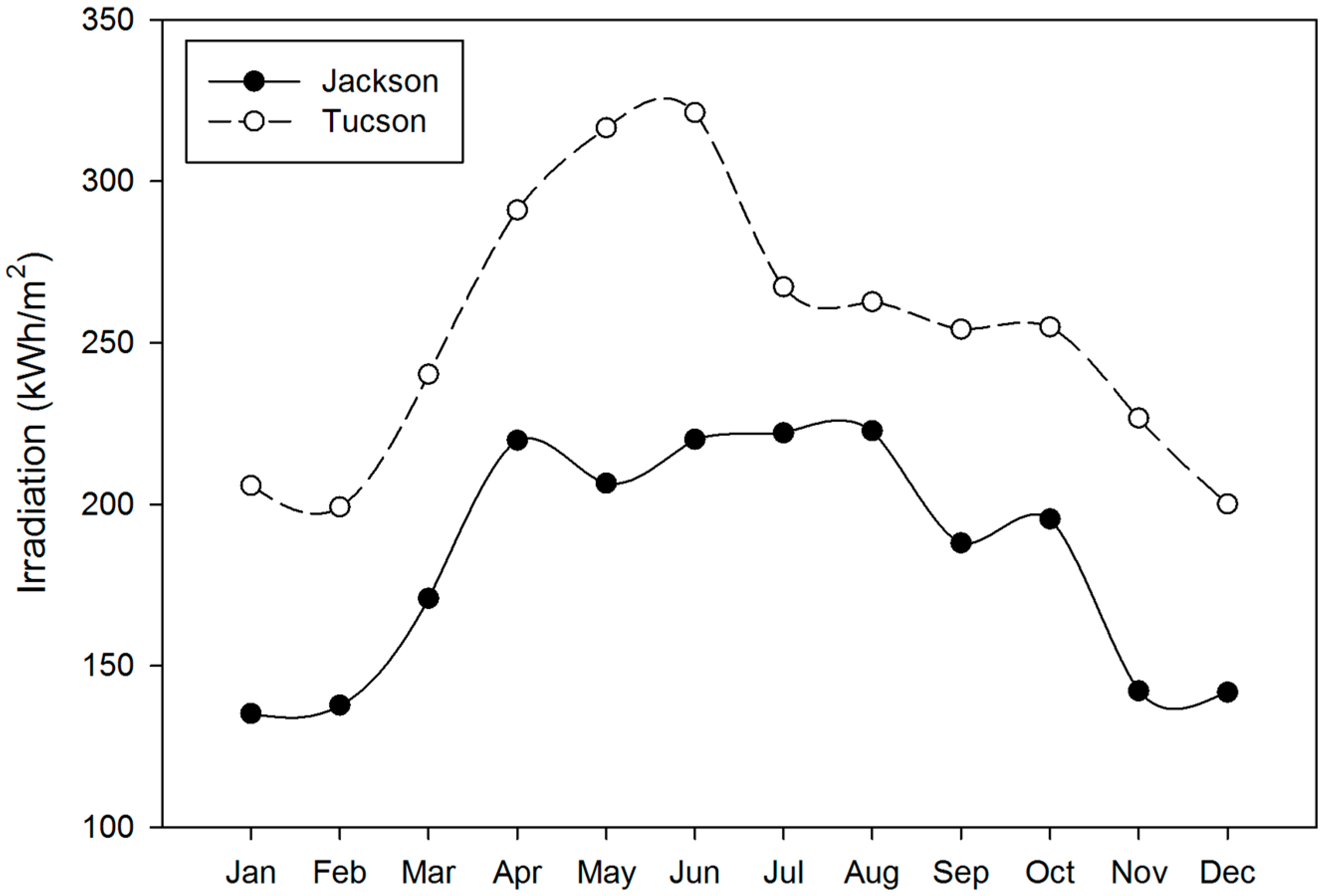
- Solar Collector (Process 4–5): This is an isobaric process where heat is supplied to the organic working fluid before the turbine inlet after the fluid exits the second pump. The flat plate solar collector replaces the evaporator in a typical R-ORC. The solar collector heat transfer rate into the working fluid follows:where is the enthalpy of the working fluid at the exit of the solar collector.The heat transfer rate from the solar collector can also be expressed as a function of irradiation:where is the solar collector efficiency, is irradiation, and is the collector area.The solar collector efficiency is determined using the relationship below:where is the y-intercept and is slope. These two terms are provided by the manufacturer or a third party certification. In the proposed model, m = 4.910 W/m2·°C and yint = 0.706 [38]. The equation for solar collector efficiency is the Hottel-Whiller-Bliss equation [39] where and correspond to:where is the collector heat removal factor, is the transmissivity of the glass cover plates, is the absorptivity of the absorber plate, and is the losses due to conduction and radiation.The irradiation values can be determined using the following equation:where is the total irradiation, is the direct normal irradiation, is the incidence angle, is the diffuse horizontal irradiation, is the surface tilt angle, is the total horizontal irradiation, and is the ground reflectance. Direct normal irradiation, diffuse horizontal irradiation, and total horizontal irradiation can be found in TMY3 data from the National Renewable Energy Laboratory [40]. The value for ground reflectance used in the paper is 0.2 which was taken from literature [41]. The incidence angle and surface tilt angle are dependent on the solar collector configuration (placement). In this study the solar collectors were modeled to be 2 axis tracking solar collectors. This gives the maximum solar irradiation. A two axis tracking system maintains the incidence angle at zero. The two axis tracking system leads to the following surface tilt equation:where is the solar altitude which is given by [41]:where is latitude, is declination, and is the hour angle. Declination can be found by using the following equation [42]:where is the day of the year.The exergy destruction rate of the solar collector is:where is the exergy rate due to the heat input to the solar collector and is the exergy rate of State 5.The change in exergy rate across the solar collector is found by:where is the entropy of the working fluid at the collector exit.The exergy rate of the solar collector can be estimated as:where is the solar radiation temperature which is assumed to be 6000 K [43].
- d.
- Turbine (Process 5–6, 7): The power of the two stage turbine is determined by:where is the power of the ideal turbine, is the turbine isentropic efficiency, and are the enthalpies of the working fluid for the exit of the first stage of the turbine for the real and ideal cases respectively, and and are the enthalpies of the working fluid of the outlet of the second stage of the turbine for the real and ideal cases, respectively.The exergy destruction rate of the turbine is expressed as:where is the exergy rate of the turbine and and are the exergy rates for State 6 and State 7, respectively.The change in exergy rates from the inlet to the outlets of the turbine is:where and are the entropy values at State 6 and 7, respectively.The turbine exergy rate is:
- e.
- Open feed organic fluid heater (Process 6, 2–3): The extraction fraction is defined as:where is the mass flow rate of the working fluid at the exit of the first stage of the turbine.The open feed organic fluid heater exergy destruction rate is determined by:The exergy balance is:
- f.
- Condenser (Process 7–1): The heat transfer rate leaving the condenser follows:The exergy destruction rate of the condenser is:where is the exergy rate of the condenser.The exergy balance across the condenser is given by:The exergy rate of the condenser is given by the following equation:where is the low temperature heat sink which is assumed to be 303 K.
- g.
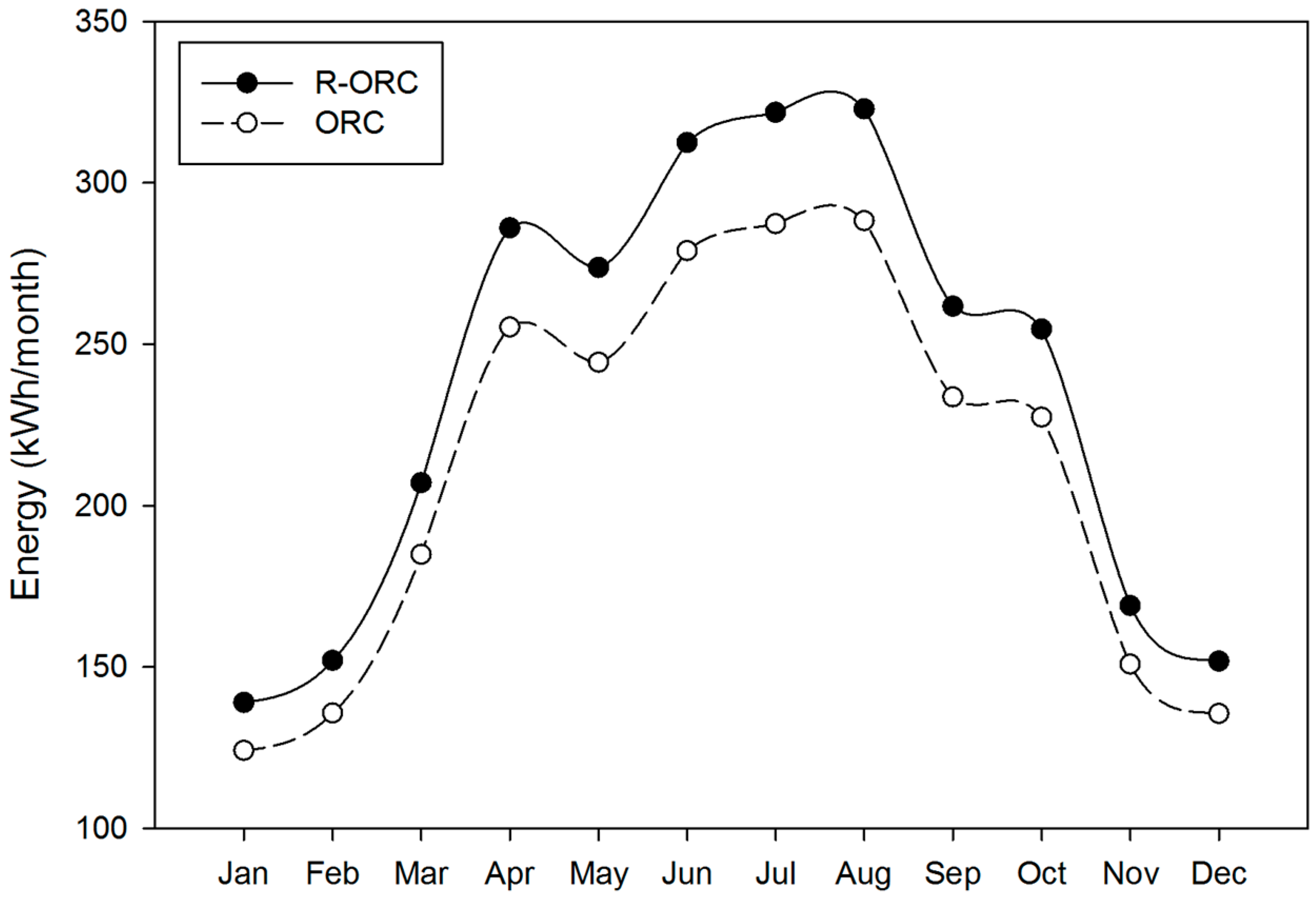
- R-ORC Net Power: The equation for the net power of the R-ORC is:
- h.
- R-ORC Efficiencies: The R-ORC thermal efficiency and R-ORC exergetic efficiency can be expressed as:where and are the exergy of the products and the exergy input to the ORC. can be estimated as:
- i.
- R-ORC Component Exergetic Efficiencies: The exergetic efficiency of each component of the R-ORC can be found by defining exergetic efficiency as the used exergy divided by the available exergy for each component. Equations (36) through (41) define each component’s exergetic efficiency:The contribution of each component to the total exergy destruction rate of the R-ORC can be estimated as:where represents the exergy destruction for each component and is the total exergy destruction rate of the R-ORC system:
- j.
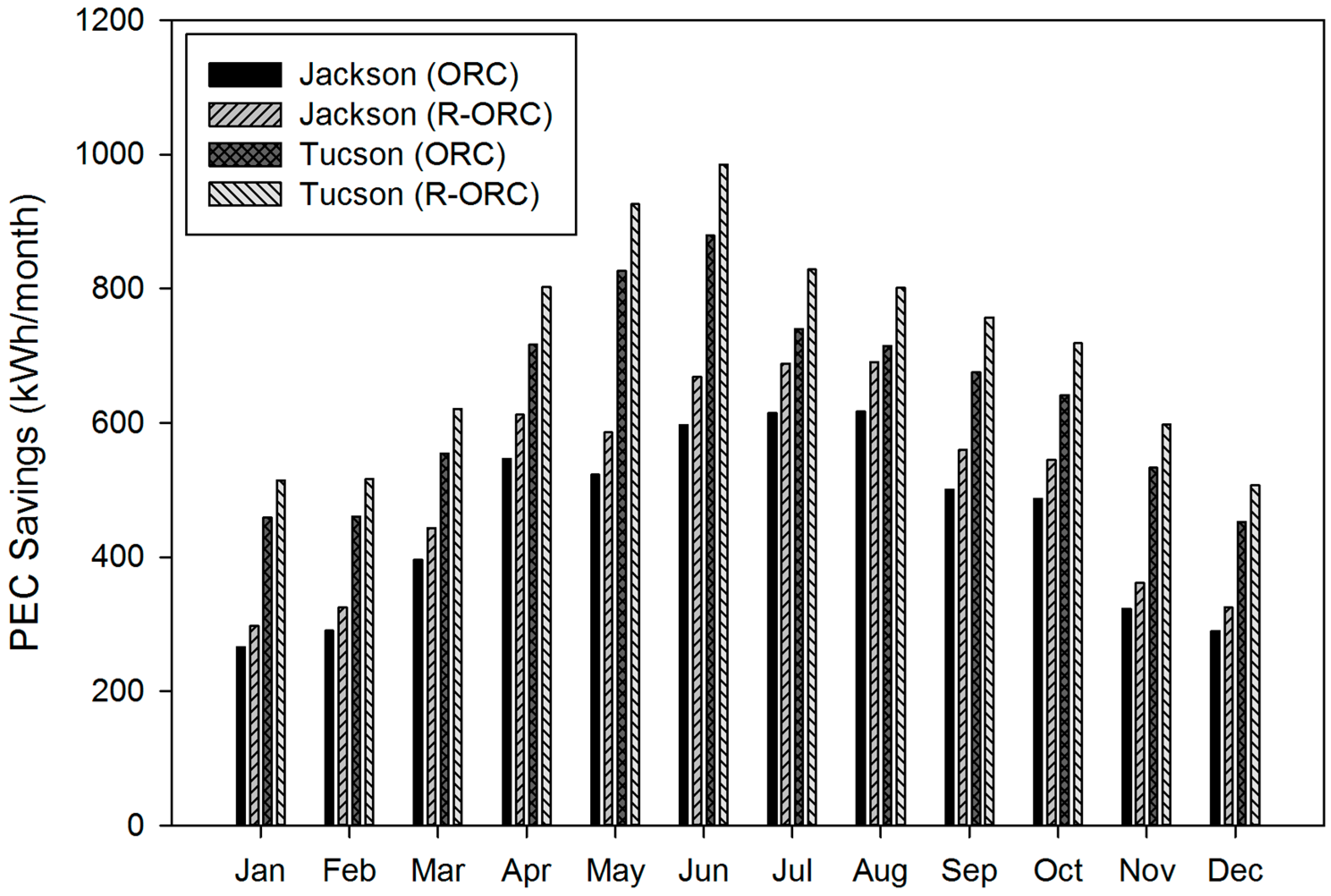
- Primary Energy Consumption (PEC) Savings: Generating electricity on site using solar energy instead of purchasing electricity from the grid results in PEC savings and can be estimated by subtracting the PEC from the R-ORC ( from the PEC from the conventional system ( as follows:where is the PEC savings, is the site-to-source conversion factor for electricity (grid purchase), which varies depending on location [23,44], and is the site-to-source conversion factor for electricity (solar), which was chosen to have a value of 1 [45,46].
- k.
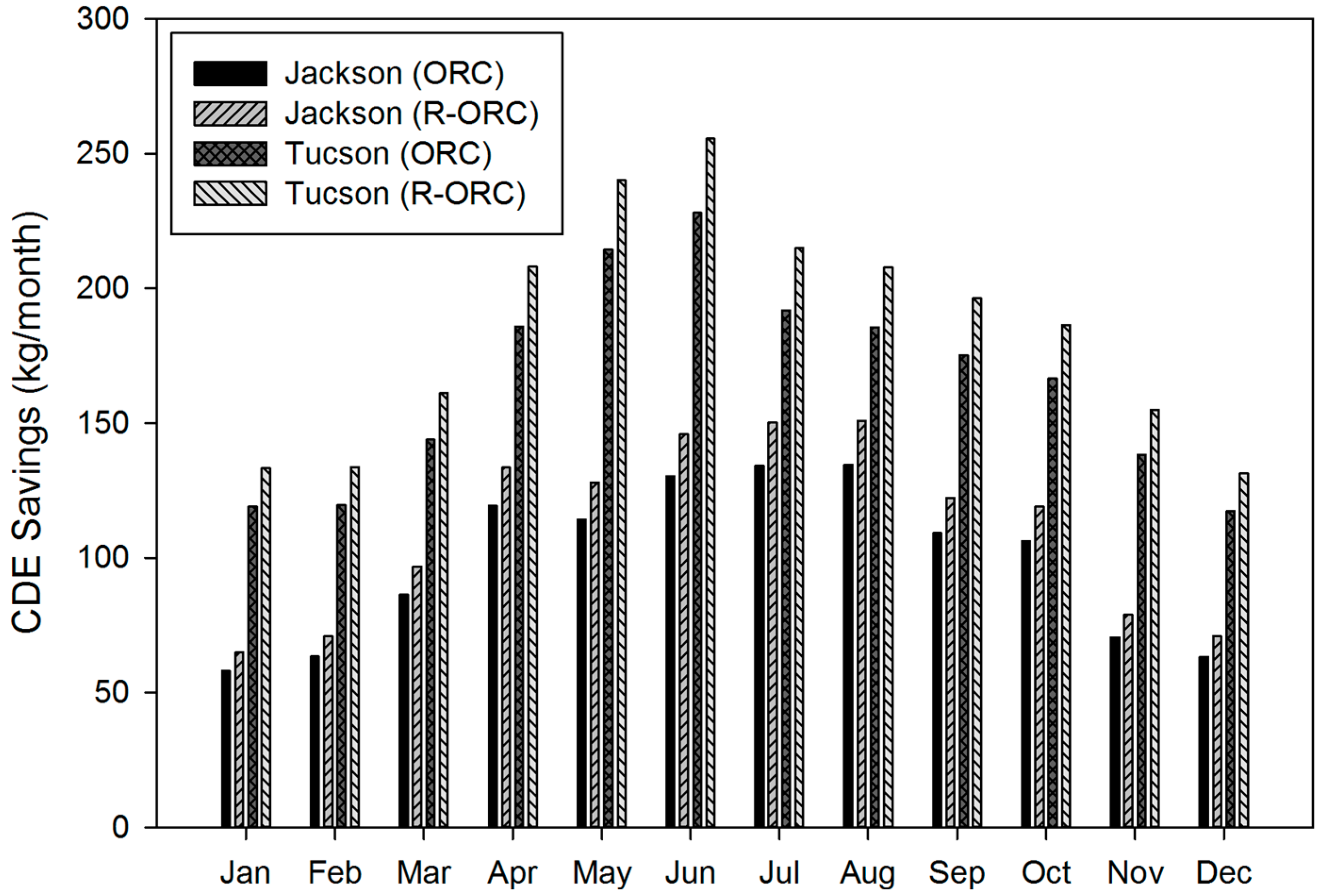
- Carbon Dioxide Emission (CDE) Savings: Since the R-ORC utilizes solar energy, there are no CDE associated with the electricity generation. This results in CDE savings when compared to purchasing electricity from the grid. The CDE savings can be found by subtracting the CDE from the R-ORC ( from the CDE from the conventional system ( as follows:where is the CDE savings and is the carbon dioxide emissions factor for electricity which is location dependent [47].
- l.
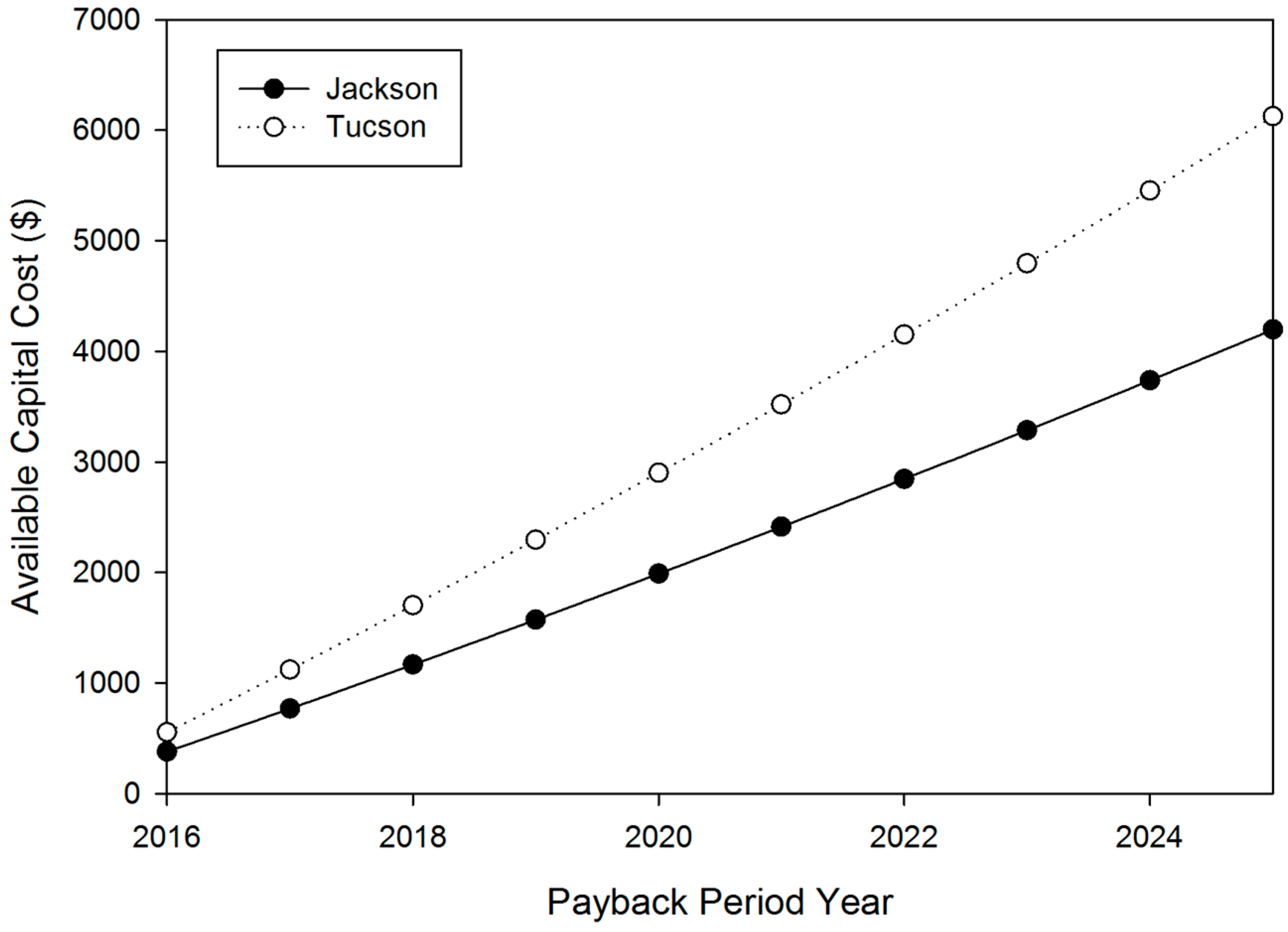
- Cost Savings and Available Capital Cost: Available yearly capital cost (ACC) is a means to determine the maximum capital cost for a given payback period based on the cost of purchased electricity from the grid. It is based on the purchased electricity savings that result from using the solar powered R-ORC to generate electricity. The available capital cost can indicate the feasibility of implementing a solar powered ORC for a specific location. The following equation determines the cost savings and maximum capital cost available depending on the desired payback period:where is the yearly forecasted cost of electricity and is the desired payback period. The cost of electricity is forecasted by plotting the average retail price of residential electricity from 2004 to 2015 [48] and performing a linear regression to estimate the future average retail price.
3. Results and Discussion
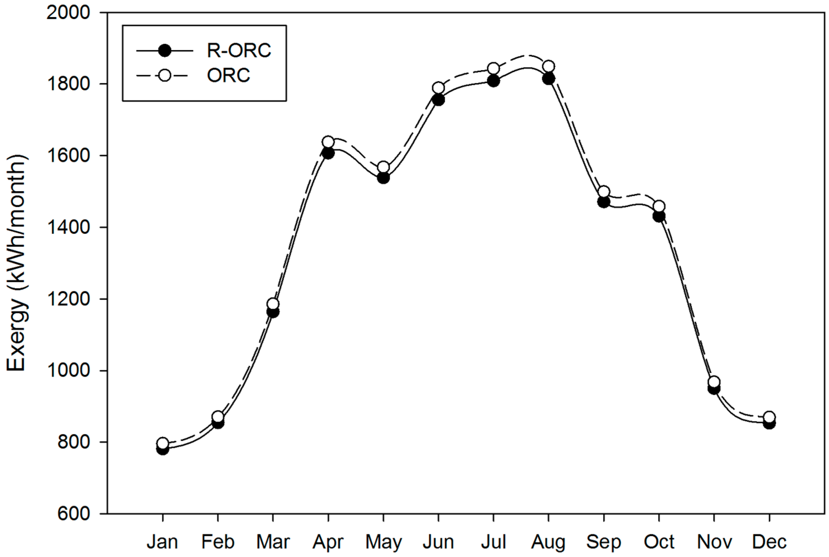
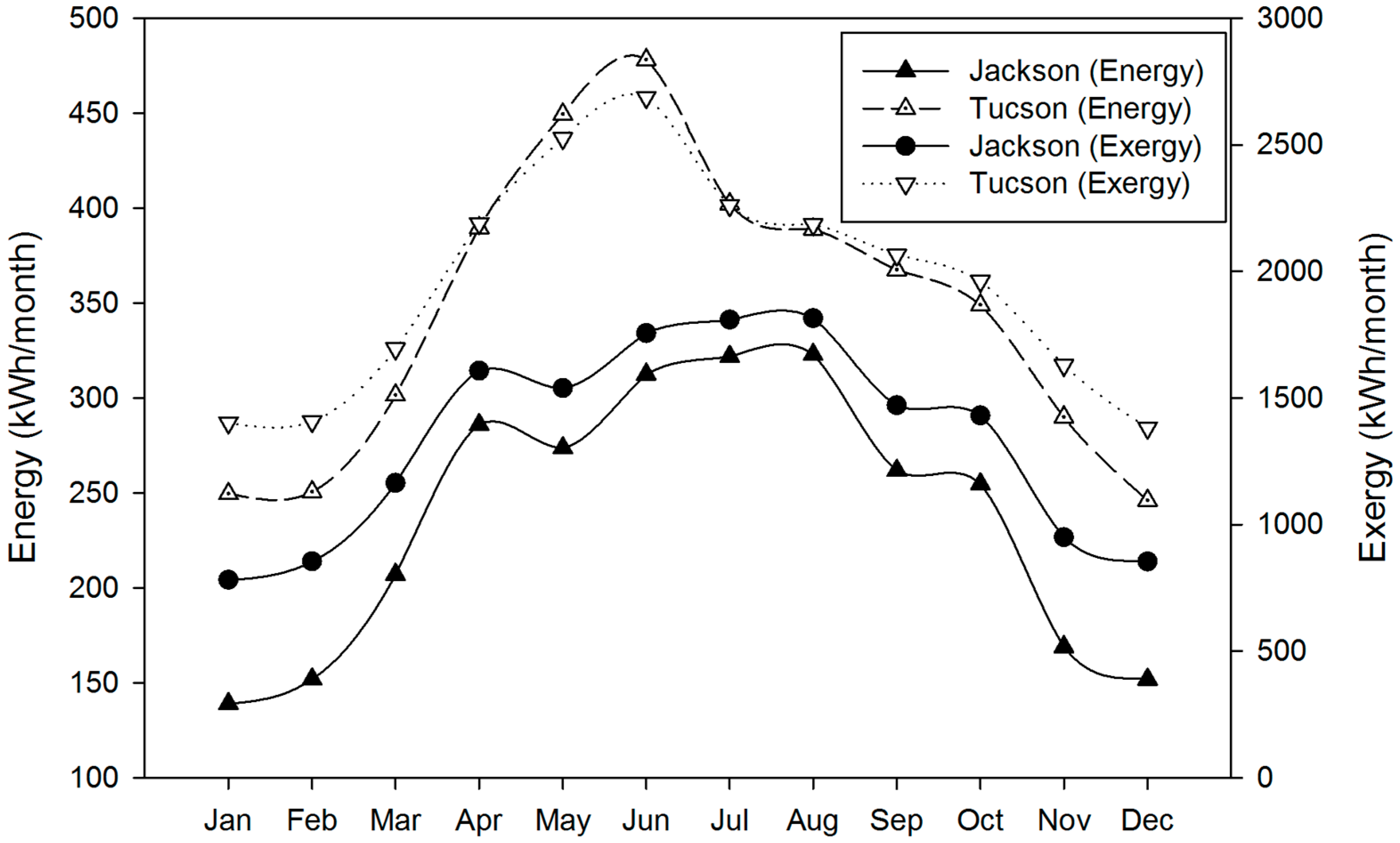
3.1. System Performance
3.2. Primary Energy Consumption and Carbon Dioxide Emissions
3.3. Available Capital Cost
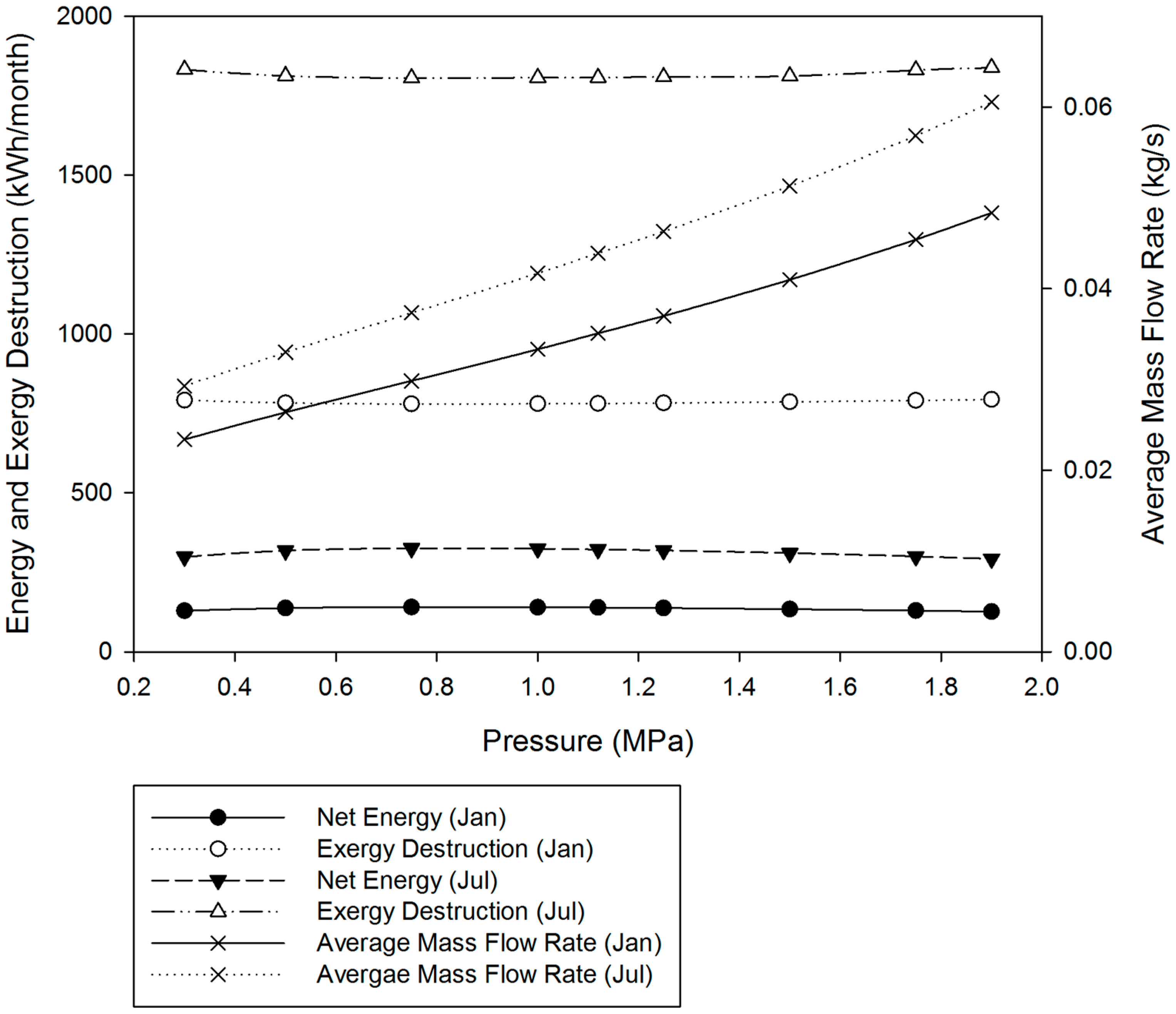
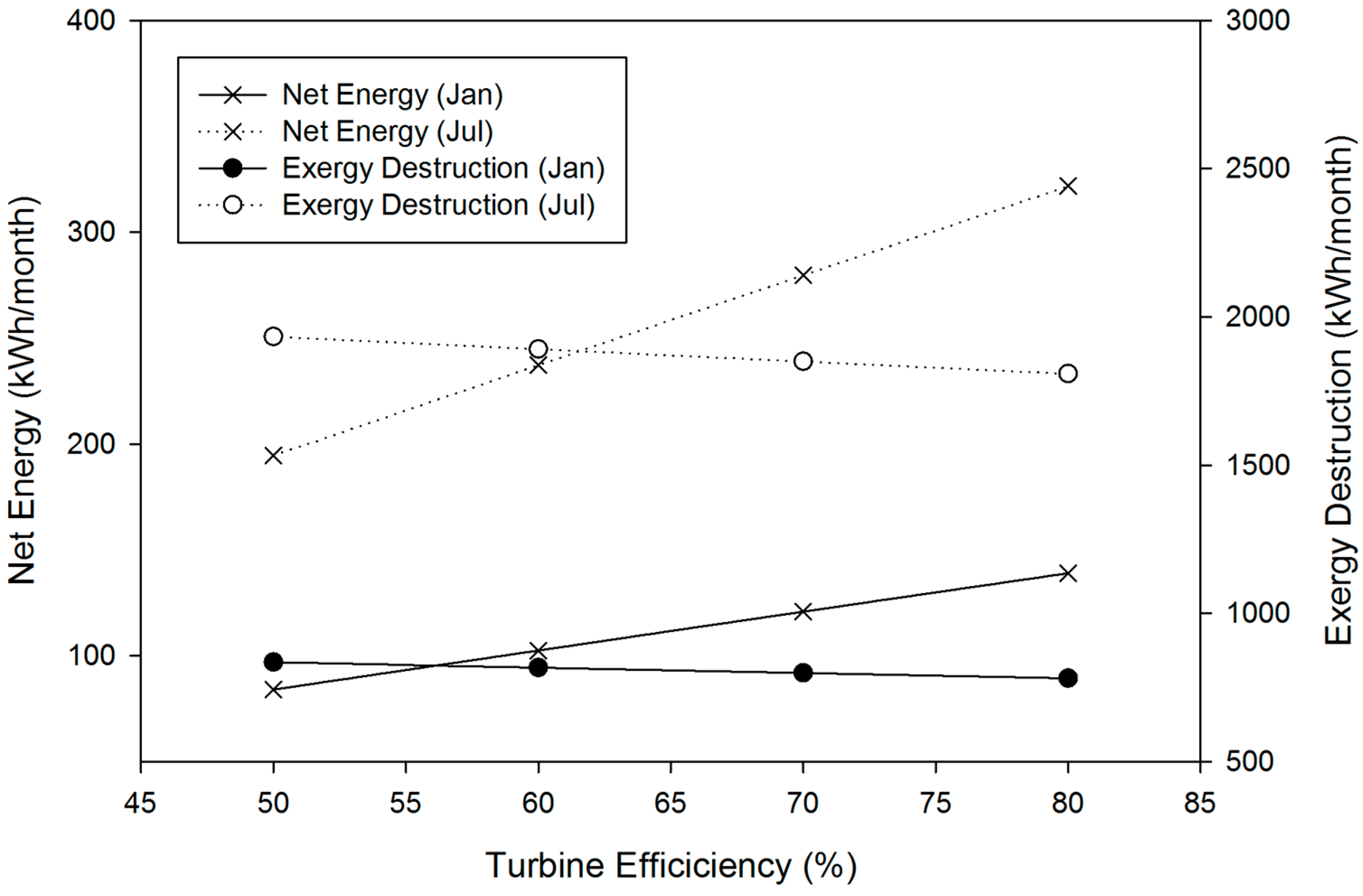
3.4. Parametric Analysis
4. Conclusions
Author Contributions
Conflicts of Interest
References
- Fang, F.; Wei, L.; Liu, J.; Zhang, J.; Hou, G. Complementary configuration and operation of a CCHP-ORC system. Energy 2012, 46, 211–220. [Google Scholar] [CrossRef]
- Guo, T.; Wang, H.X.; Zhang, S.J. Fluids and parameters optimization for a novel cogeneration system driven by low-temperature geothermal sources. Energy 2011, 36, 2639–2649. [Google Scholar] [CrossRef]
- Hung, T.-C. Waste heat recovery of organic Rankine cycle using dry fluids. Energy Convers. Manag. 2001, 42, 539–553. [Google Scholar] [CrossRef]
- Hettiarachchi, H.D.M.; Golubovic, M.; Worek, W.M.; Ikegami, Y. Optimum design criteria for an Organic Rankine cycle using low-temperature geothermal heat sources. Energy 2007, 32, 1698–1706. [Google Scholar] [CrossRef]
- Quoilin, S.; Orosz, M.; Hemond, H.; Lemort, V. Performance and design optimization of a low-cost solar organic Rankine cycle for remote power generation. Sol. Energy 2011, 85, 955–966. [Google Scholar] [CrossRef]
- Hung, T.; Wang, S.; Kuo, C.; Pei, B.; Tsai, K. A study of organic working fluids on system efficiency of an ORC using low-grade energy sources. Energy 2010, 35, 1403–1411. [Google Scholar] [CrossRef]
- Lakew, A.A.; Bolland, O. Working fluids for low-temperature heat source. Appl. Therm. Eng. 2010, 30, 1262–1268. [Google Scholar] [CrossRef]
- Mago, P.J.; Chamra, L.M.; Somayaji, C. Performance analysis of different working fluids for use in organic Rankine cycles. Proc. Inst. Mech. Eng. Part A J. Power Energy 2007, 221, 255–264. [Google Scholar] [CrossRef]
- Saleh, B.; Koglbauer, G.; Wendland, M.; Fischer, J. Working fluids for low-temperature organic Rankine cycles. Energy 2007, 32, 1210–1221. [Google Scholar] [CrossRef]
- Wang, E.; Zhang, H.; Fan, B.; Ouyang, M.; Zhao, Y.; Mu, Q. Study of working fluid selection of organic Rankine cycle (ORC) for engine waste heat recovery. Energy 2011, 36, 3406–3418. [Google Scholar] [CrossRef]
- Bao, J.; Zhao, L. A review of working fluid and expander selections for organic Rankine cycle. Renew. Sustain. Energy Rev. 2013, 24, 325–342. [Google Scholar] [CrossRef]
- Rayegan, R.; Tao, Y. A procedure to select working fluids for Solar Organic Rankine Cycles (ORCs). Renew. Energy 2011, 36, 659–670. [Google Scholar] [CrossRef]
- Mago, P.J.; Chamra, L.M.; Srinivasan, K.; Somayaji, C. An examination of regenerative organic Rankine cycles using dry fluids. Appl. Therm. Eng. 2008, 28, 998–1007. [Google Scholar] [CrossRef]
- Branchini, L.; de Pascale, A.; Peretto, A. Systematic comparison of ORC configurations by means of comprehensive performance indexes. Appl. Therm. Eng. 2013, 61, 129–140. [Google Scholar] [CrossRef]
- Soffiato, M.; Frangopoulos, C.A.; Manente, G.; Rech, S.; Lazzaretto, A. Design optimization of ORC systems for waste heat recovery on board a LNG carrier. Energy Convers. Manag. 2015, 92, 523–534. [Google Scholar] [CrossRef]
- Feng, Y.; Zhang, Y.; Li, B.; Yang, J.; Shi, Y. Sensitivity analysis and thermoeconomic comparison of ORCs (organicRankine cycles) for low temperature waste heat recovery. Energy 2015, 82, 664–677. [Google Scholar] [CrossRef]
- Le, V.L.; Feidt, M.; Kheiri, A.; Pelloux-Prayer, S. Performance optimization of low-temperature power generation by supercritical ORCs (organic Rankine cycles) using low GWP (global warming potential) working fluids. Energy 2014, 67, 513–526. [Google Scholar] [CrossRef]
- Meinel, D.; Wieland, C.; Spliethoff, H. Economic comparison of ORC (Organic Rankine cycle) processes at different scales. Energy 2014, 74, 694–706. [Google Scholar] [CrossRef]
- Roy, J.P.; Misra, A. Parametric optimization and performance analysis of a regenerative Organic Rankine Cycle using R-123 for waste heat recovery. Energy 2012, 39, 227–235. [Google Scholar] [CrossRef]
- Li, M.; Wang, J.; He, W.; Gao, L.; Wang, B.; Ma, S.; Dai, Y. Construction and preliminary test of a low-temperature regenerative Organic Rankine Cycle (ORC) using R123. Renew. Energy 2013, 57, 216–222. [Google Scholar] [CrossRef]
- Mago, P.J.; Srinivasan, K.K.; Chamra, L.M.; Somayaji, C. An examination of exergy destruction in organic Rankine cycles. Int. J. Energy Res. 2008, 32, 926–938. [Google Scholar] [CrossRef]
- Imran, M.; Park, B.S.; Kim, H.J.; Lee, D.H.; Usman, M.; Heo, M. Thermo-economic optimization of Regenerative Organic Rankine Cycle for waste heat recovery applications. Energy Convers. Manag. 2014, 87, 107–118. [Google Scholar] [CrossRef]
- Fumo, N.; Chamra, L.M. Analysis of combined cooling, heating, and power systems based on source primary energy consumption. Appl. Energy 2010, 87, 2023–2030. [Google Scholar] [CrossRef]
- Mago, P.J.; Hueffed, A.; Chamra, L.M. Analysis and optimization of the use of CHP-ORC systems for small commercial buildings. Energy Build. 2010, 42, 1491–1498. [Google Scholar] [CrossRef]
- Lecompte, S.; Huisseune, H.; van den Broek, M.; de Schampheleire, S.; de Paepe, M. Part load based thermo-economic optimization of the Organic Rankine Cycle (ORC) applied to a combined heat and power (CHP) system. Appl. Energy 2013, 111, 871–881. [Google Scholar] [CrossRef]
- Calise, F.; Capuozzo, C.; Carotenuto, A.; Vanoli, L. Thermoeconomic analysis and off-design performance of an organic Rankine cycle powered by medium-temperature heat sources. Sol. Energy 2014, 103, 595–609. [Google Scholar] [CrossRef]
- Quoilin, S.; Declaye, S.; Tchanche, B.F.; Lemort, V. Thermo-economic optimization of waste heat recovery Organic Rankine Cycles. Appl. Therm. Eng. 2011, 31, 2885–2893. [Google Scholar] [CrossRef]
- Feng, Y.; Zhang, Y.; Li, B.; Yang, J.; Shi, Y. Comparison between regenerative organic Rankine cycle (RORC) and basic organic Rankine cycle (BORC) based on thermoeconomic multi-objective optimization considering exergy efficiency and levelized energy cost (LEC). Energy Convers. Manag. 2015, 96, 58–71. [Google Scholar] [CrossRef]
- Tempesti, D.; Manfrida, G.; Fiaschi, D. Thermodynamic analysis of two micro CHP systems operating with geothermal and solar energy. Appl. Energy 2012, 97, 609–617. [Google Scholar] [CrossRef]
- Wang, X.; Zhao, L.; Wang, J.; Zhang, W.; Zhao, X.; Wu, W. Performance evaluation of a low-temperature solar Rankine cycle system utilizing R245fa. Sol. Energy 2010, 84, 353–364. [Google Scholar] [CrossRef]
- Calise, F.; d’Accadia, M.D.; Vicidomini, M.; Scarpellino, M. Design and simulation of a prototype of a small-scale solar CHP system based on evacuated flat-plate solar collectors and Organic Rankine Cycle. Energy Convers. Manag. 2015, 90, 347–363. [Google Scholar] [CrossRef]
- Rayegan, R.; Tao, Y.X. Optimal Collector Type and Temperature in a Solar Organic Rankine Cycle System for Building-Scale Power Generation in Hot and Humid Climate. J. Sol. Energy Eng. 2013, 135. [Google Scholar] [CrossRef]
- Marion, M.; Voicu, I.; Tiffonnet, A.L. Study and optimization of a solar subcritical organic Rankine cycle. Renew. Energy 2012, 48, 100–109. [Google Scholar] [CrossRef]
- Wang, M.; Wang, J.; Zhao, Y.; Zhao, P.; Dai, Y. Thermodynamic analysis and optimization of a solar-driven regenerative organic Rankine cycle (ORC) based on flat-plate solar collectors. Appl. Therm. Eng. 2013, 50, 816–825. [Google Scholar] [CrossRef]
- Pei, G.; Li, J.; Ji, J. Analysis of low temperature solar thermal electric generation using regenerative Organic Rankine Cycle. Appl. Therm. Eng. 2010, 30, 998–1004. [Google Scholar] [CrossRef]
- Spayde, E.; Mago, P.J. Evaluation of a solar-powered organic Rankine cycle using dry organic working fluids. Cogent Eng. 2015, 2. [Google Scholar] [CrossRef]
- Xu, G.; Song, G.; Zhu, X.; Gao, W.; Li, H.; Quan, Y. Performance evaluation of a direct vapor generation supercritical ORC system driven by linear Fresnel reflector solar concentrator. Appl. Therm. Eng. 2015, 80, 196–204. [Google Scholar] [CrossRef]
- Alternate Energy Technologies. Certified Solar Collector. Available online: http://www.aetsolar.com/certifications.php (accessed on 1 April 2014).
- Hodge, B.K. Alternative Energy Sources and Applications; Wiley: New York, NY, USA, 2009. [Google Scholar]
- National Solar Radiation Data Base. Available online: http://rredc.nrel.gov/solar/old_data/nsrdb/1991-2005/tmy3/ (accessed on 4 April 2014).
- Solar Energy Research Institute. Engineering Principles and Concepts for Active Solar Systems; CRC Press: Springfield, VA, USA, 1987. [Google Scholar]
- Duffie, J.A.; Beckman, W.A. Solar Engineering of Thermal Processes; John Wiley & Sons: New York, NY, USA, 1980. [Google Scholar]
- Hepbasli, A. A key review on exergetic analysis and assessment of renewable energy resources for a sustainable future. Renew. Sustain. Energy Rev. 2008, 12, 593–661. [Google Scholar] [CrossRef]
- Czachorski, M.; Leslie, N. Source Energy and Emission Factors for Building Energy Consumption. Available online: https://www.aga.org/codes-and-standards-research-consortium (accessed on 15 September 2014).
- Energy Star. Energy Star Portfolio Manager Technical Reference Source Energy. Available online: https://portfoliomanager.energystar.gov/pdf/reference/Source%20Energy.pdf (accessed on 12 July 2016).
- Deru, M.; Torcellini, P. Source Energy and Emission Factors for Energy Use in Buildings. Available online: www.nrel.gov/docs/fy07osti/38617.pdf (accessed on 15 September 2014).
- Power Profiler. Available online: http://oaspub.epa.gov/powpro/ept_pack.charts (accessed on 20 August 2014).
- U.S. Energy Information Administration. Electric Power Monthly with Data for March 2016. Available online: http://www.eia.gov/electricity/monthly/current_year/may2016.pdf (accessed on 13 July 2016).
- Lemmon, E.W.; Huber, M.L.; McLinden, M.O. REFPROP: Reference Fluid Thermodynamic and Transport Properties; Version 9.1; National Institute of Standards and Technology: Gaithersburg, MD, USA, 2013. [Google Scholar]


| Fluid | Critical Pressure (MPa) | Low Pressure (MPa) | Low Temperature (°C) | Intermediate Pressure (MPa) | High Pressure (MPa) | High Temperature (°C) |
|---|---|---|---|---|---|---|
| RC318 | 2.7775 | 0.36556 | 30 | 1.18278 | 2 | 98.75 |
| R236fa | 3.2 | 0.32101 | 30 | 1.160505 | 2 | 101.47 |
| R236ea | 3.502 | 0.24437 | 30 | 1.122185 | 2 | 111.65 |
| R227ea | 2.926 | 0.52866 | 30 | 1.26433 | 2 | 83.423 |
| R218 | 2.671 | 0.99165 | 30 | 1.495825 | 2 | 59.094 |
| Thermal Efficiency | Exergy Efficiency | |||
|---|---|---|---|---|
| Fluid | Basic ORC | R-ORC | Basic ORC | R-ORC |
| RC318 | 10.10 | 11.44 | 10.82 | 12.25 |
| R236fa | 11.16 | 12.50 | 11.95 | 13.39 |
| R236ea | 12.40 | 13.89 | 13.28 | 14.87 |
| R227ea | 8.81 | 9.86 | 9.44 | 10.56 |
| R218 | 5.16 | 5.65 | 5.53 | 6.05 |
| Net Energy Produced (kWh/Year) | Total Exergy Destroyed (kWh/Year) | |||||
|---|---|---|---|---|---|---|
| Fluid | Basic ORC | R-ORC | % Increase | Basic ORC | R-ORC | % Decrease |
| RC318 | 2074 | 2349 | 13.27 | 16,796 | 16,525 | 1.61 |
| R236fa | 2291 | 2567 | 12.07 | 16,583 | 16,311 | 1.64 |
| R236ea | 2546 | 2852 | 12.01 | 16,331 | 16,031 | 1.84 |
| R227ea | 1809 | 2024 | 11.88 | 17,056 | 16,845 | 1.24 |
| R218 | 1060 | 1160 | 9.42 | 17,794 | 17,695 | 0.55 |
| Fluid | Π Pump 1 (%) | Π Pump 2 (%) | Π Solar (%) | Π Turbine (%) | Π Condenser (%) | Π Open Feed Organic Fluid Heater (%) |
|---|---|---|---|---|---|---|
| RC318 | 0.13 | 0.22 | 92.54 | 3.56 | 0.86 | 2.69 |
| R236fa | 0.10 | 0.16 | 92.85 | 3.89 | 0.37 | 2.63 |
| R236ea | 0.09 | 0.15 | 91.76 | 4.22 | 0.66 | 3.12 |
| R227ea | 0.11 | 0.16 | 94.67 | 3.11 | 0.29 | 1.67 |
| R218 | 0.12 | 0.22 | 96.87 | 1.95 | 0.16 | 0.67 |
© 2017 by the authors; licensee MDPI, Basel, Switzerland. This article is an open access article distributed under the terms and conditions of the Creative Commons Attribution (CC-BY) license (http://creativecommons.org/licenses/by/4.0/).
Share and Cite
Spayde, E.; Mago, P.J.; Cho, H. Performance Evaluation of a Solar-Powered Regenerative Organic Rankine Cycle in Different Climate Conditions. Energies 2017, 10, 94. https://doi.org/10.3390/en10010094
Spayde E, Mago PJ, Cho H. Performance Evaluation of a Solar-Powered Regenerative Organic Rankine Cycle in Different Climate Conditions. Energies. 2017; 10(1):94. https://doi.org/10.3390/en10010094
Chicago/Turabian StyleSpayde, Emily, Pedro J. Mago, and Heejin Cho. 2017. "Performance Evaluation of a Solar-Powered Regenerative Organic Rankine Cycle in Different Climate Conditions" Energies 10, no. 1: 94. https://doi.org/10.3390/en10010094