Robustness Area Technique Developing Guidelines for Power System Restoration

Abstract

This paper proposes a novel energy based technique called the Robustness Area (RA) technique that measures power system robustness levels, as a helper for planning Power System Restorations (PSRs). The motivation is on account of the latest blackouts in Brazil, where the local Independent System Operator (ISO) encountered difficulties related to circuit disconnections during the restoration. The technique identifies vulnerable and robust buses, pointing out system areas that should be firstly reinforced during PSR, in order to enhance system stability. A Brazilian power system restoration area is used to compare the guidelines adopted by the ISO with a more suitable new plan indicated by the RA tool. Active power and reactive power load margin and standing phase angle show the method efficiency as a result of a well balanced system configuration, enhancing the restoration performance. Time domain simulations for loop closures and severe events also show the positive impact that the proposed tool brings to PSRs.

1. Introduction

Power systems are developed to perform with high reliability, even though, critical outages may trigger a cascade of events ending up in a blackout. Black starts have been a major concern since the early 1980s [1], when systems became interconnected and blackouts turned into a wide-area event. For example, on August 2003, three transmission lines touched overgrown trees, leading to a series of events that caused the system collapse affecting over 50 million people [2] in North America. During this event, a total of 265 power plants were disconnected, corresponding to 61,800 MW. If events similar to this may happen, their impacts can be diminished by a fast and reliable power system restoration.

The Power System Restoration (PSR) in Brazil is based on hydro Generator Units (GUs) [3], providing a short black start period with renewable energy sources. It is, however, a continental sized power system with long high voltage transmission lines connecting 1076 power plants. On account of its complexity, the national Independent System Operator (ISO) adopted a two-phase restoration procedure: Fluent Phase (FP) (local), and Coordinated Phase (CP) (wide area). During the FP, black start utilities start up a minimum number of GUs, forming small electrical islands. Each island is responsible for picking-up a predetermined load amount. It is called Fluent because power companies can follow a script containing all the steps to perform the local restoration without intervention from the ISO. Afterwards, the CP takes place and all instructions are sent out from the ISO to local companies [4,5], connecting islands to each other. A full description of the Brazilian system restoration procedure is presented in [6], where FP and CP are further explained.

The aforementioned two-phase procedure is well-established; however, during the last major events (especially the 2009 blackout), the ISO faced circuit disconnections throughout the CP [7,8]. The full report on the 2009 blackout in Brazil is presented in [9]. The unsuccessful reconnections reveal fragile points and call for a demand of studies on the field of stability and reliability to re-design the black start philosophy [10], towards reducing the impact caused by blackouts. The following passage is removed from [8], where authors monitored the whole blackout and restoration procedure during the 2009 major outage:

“The South–Southeast interconnection tripped again at 02:20:00 (Figure 20) and a new attempt to reconnect the two subsystems was made at 02:23:28 (second 328 in Figure 21), but 1.5 s later, the interconnection tripped again. It caused oscillations in the BIPS (Brazilian Interconnected Power System), as shown in Figure 22, where the angle difference between UFPA (Federal University of Pará) (North) and UNIFEI (Federal University of Itajubá) (Southeast), soon after the reconnection attempt, is shown”.

Unsuccessful reconnections during PSRs have also been reported in many different power systems, as described by the two following passages [11]:

“Resynchronizing of the interconnection loop was not accomplished in accordance with the interconnection procedures. The first tie which was closed between the northern and southern islands was a 115 kV line, which promptly opened on overload”.

“There were several unsuccessful closures before the island was finally reconnected to the remainder of the interconnection. Efforts need to be made to better coordinate restoration procedures among the many dispatch offices. Switching to return the system to normal was completed in one hour and two minutes following the cascading disturbance”.

Planning PSRs requires expertise to deal with limitations and constraints, where poor voltage profile and frequency control problems are recurrent [12,13,14]. Such issues are mainly caused by thermal limitations on GUs and transmission lines stability contrains. The reduced number of GUs during this procedure is associated with a low inertia provision scenario [15], causing dynamic stability issues; and the few transmission lines connected can reduce the system reliability [16]. Attempting to overcome the PSR issues, several decision making techniques have been created based on different metrics [17,18,19,20,21,22]; however, few are dedicated to voltage stability assessments during this period. This work pays special attention to this issue, though voltage stability is treated as a robustness index. Hence, rather than considering voltage stability as a final purpose, it is considered as a decision helper in the CP. Due to this, the energy function based analysis is used to identify the best plan for PSR that can be used for static and dynamic analyses.

The energy function is a powerful tool [23,24] that can be used to infer system stability conditions. Such ability motivates the usage of a novel energy function tool that identifies system areas according to its strength level, pointing out regions to be reinforced firstly during restoration. The method also analyses system operations during restorations, such as load variations, transmission line reconnections, and loop closures. The methodology output is the impact that such operations cause and the feasibility of these actions. Taking into account the difficulties faced by the ISO during the latest restoration events, in which disconnections delayed the procedure, the Robustness Area (RA) technique is used to re-plan the Brazilian power system restoration. A real case scenario is taken for studies and the RA technique is used to create a new step in the restoration. This plan is compared with the one adopted by the ISO under static and dynamic approaches, showing the ability of the the proposed tool in planning the CP.

The RA definition is addressed in Section 2. A robustness area-based based guideline for the Brazilian power system PSRs is presented in Section 3. Voltage and dynamic assessments are carried out in Section 4 to investigate the impact caused by the usage of this novel tool in the restoration procedure, where results are presented. Section 5 presents the conclusion.

2. The Robustness Assessment

2.1. The Voltage Stability Problem

The first step in planning a restoration procedure is a static analysis, where the power flow is calculated, and violations are pointed out. During this stage, voltage stability tools are used to infer power system stability conditions, establishing boundaries between safe and unsafe regions. A power system is considered voltage stable when it is capable of keeping the voltage profile steady after being subjected to a disturbance. In this sense, the system is voltage stable when control actions produce coherent results. Otherwise, when reverse results are observed, the system is considered unstable. Figure 1 depicts such a situation with the help of a QV curve, that shows the voltage sensitivity to variations in reactive power injection. Region A identifies voltage Stable Equilibrium Points (SEPs) for a particular load bus, where an increase in the reactive power injection is associated with a voltage magnitude increase [25], i.e., $\frac{\partial Q}{\partial V}>0$. The contrary occurs in Region B, which is related to Unstable Equilibrium Points (UEPs) and $\frac{\partial Q}{\partial V}<0$. $\Delta {\lambda }_Q$ stands for the reactive power margin. The basics behind the QV curve are found in [26,27].

Figure 2 depicts the voltage stability problem in a PV curve [26] that relates voltage magnitude variation in function of load increase. The upper part is the stable region, associated with SEPs. The lower part is the unstable or abnormal region, associated with UEPs, and is avoided during operation. As the system moves toward the maximum loading point $P_{\max }$, the stable solution and a particular unstable solution get closer until they merge into one on a saddle node point, and no further solutions are possible.

2.2. The Power Flow Multiple Solutions and the Voltage Collapse Mechanism

In the steady state voltage stability approach, the system is driven towards the collapse point $P_{\max }$, on a time scale of minutes to hours (“quasistatic” manner), due to gradual changes in load/generation injections. In the static approach, the power system model can be reduced to the set of algebraic Equations that represent the power flow problem:

$$P_i=\sum _{j=1}^n{V}_i{V}_j\left[G_{ij}cos\left({\theta }_{ij}\right)+B_{ij}sin\left({\theta }_{ij}\right)\right],$$

(1)

$$Q_i=\sum _{j=1}^n{V}_i{V}_j\left[B_{ij}sin\left({\theta }_{ij}\right)-G_{ij}cos\left({\theta }_{ij}\right)\right],$$

(2)

where: n is the number of system buses; $P_i$ and $Q_i$ are, respectively, the specified active and reactive power injections of the ith bus; $V_i$ is the voltage magnitude and ${\theta }_i$, the respective phase angle; $B_{ij}$ refers to the transfer susceptance between buses i and j, and $G_{ij}$ is related to the transfer conductance; finally, ${\theta }_{ij}$ is the angular difference between buses i and j.

The solutions of Equations (1) and (2) are associated with equilibrium points of the dynamical model that describes the power system. As the system slowly moves toward $P_{\max }$, the equilibrium points vanish because of different kinds of bifurcations. At the collapse point, the stable equilibrium point SEP and a particular type-1 UEP merge. Consequently, beyond this point, there are no equilibrium points, and the system experiences loss of stability [28]. Type-1 UEPs are associated with alternative power flow solutions that present low voltage magnitude only in a single bus or a single connected group of buses, and are referred to as the critical Low Voltage Solution (LVS), while SEPs are related to operable power flow solutions.

2.3. Voltage Stability Assessment by Means of an Energy Function

Concerning the voltage stability approach [29,30,31], the difference of potential energy between the SEP and an LVS of interest is calculated by:

$$\begin{array}{cc}\hfill \upsilon (X^s,X^u)=& -\sum _{i=1}^n{Q}_{i}ln\frac{V_i^u}{V_i^s}-\sum _{i=1}^n{P}_i\left({\theta }_i^u-{\theta }_i^s\right)\hfill \\ & {\displaystyle -\frac{1}{2}\sum _{i=1}^n\sum _{j=1}^n{V}_i^u{V}_j^u{B}_{ij}cos\left({\theta }_i^u-{\theta }_j^u\right)+\frac{1}{2}\sum _{i=1}^n\sum _{j=1}^n{V}_i^s{V}_j^s{B}_{ij}cos\left({\theta }_i^s-{\theta }_j^s\right)}\hfill \\ & {\displaystyle +\sum _{i=1}^n\sum _{j=1}^n{V}_i^s{V}_j^s{G}_{ij}cos\left({\theta }_i^s-{\theta }_j^s\right)\left({\theta }_i^u-{\theta }_i^s\right)+\sum _{i=1}^n\sum _{j=1}^n{V}_j^s{G}_{ij}cos\left({\theta }_i^s-{\theta }_j^s\right)\left(V_i^u-V_i^s\right),}\hfill \end{array}$$

(3)

where $X^s=({\theta }^s,V^s$) and $X^u=({\theta }^u,V^u)$ are, respectively, associated with the SEP and UEP.

As the system moves toward $P_{\max }$, υ tends to zero, and the energy function value serves as a measure for calculating proximity to voltage collapse this way.

There are different methodologies to calculate low voltage solutions [30,31,32,33] that rely on iterative nonlinear Equation solving methods, which may present, at any operating point, convergence problems. As a consequence, not all LVSs can be calculated. The area concerned with a particular bus i, for which an LVS does not exist, is considered invulnerable to voltage instability. To overcome this issue, the area for which an LVS does not exist can be associated with the energy measure related to a nearby bus. Besides the numerical issues associated with the low voltage solution methods, the number of system buses can have great impact on the energy methodology, since the calculations of all possible LVSs in a large system represent great effort. It is necessary to define the group of buses for which low voltage solutions must be calculated. Due to this, system reduction techniques [34] are used, and $\frac{\partial V}{\partial Q}$ sensitivities may also be combined to identify locally weak system areas.

This paper uses an alternative function for system vulnerability quantification. The proposed methodology lies on a single low voltage solution, thus, no reduction is needed. Such a solution is based on the knowledge of the critical bus, as described in the following subsection.

2.4. Robustness Evaluation

This work measures the vulnerability of the systems’ areas, hereafter called robustness level, by using an alternative function. Such alternative function is proposed by the authors in [29]. Extracting from Equation (3) the contribution related to $X^u$ for a bus i, and considering $j=1,2,\cdots ,n,j\ne i$, one obtains:

$$\begin{array}{cc}\hfill {\displaystyle E_p{(X^s,X^u)}_i=}& {\displaystyle Q_{i}ln\left(V_i^u\right)+P_i\left({\theta }_i^u\right)+\frac{1}{2}\sum _{\begin{array}{c}j=1\\ j\ne i\end{array}}^n{V}_i^u{V}_j^u{B}_{ij}cos\left({\theta }_i^u-{\theta }_j^u\right)}\hfill \\ & {\displaystyle -\sum _{\begin{array}{c}j=1\\ j\ne i\end{array}}^n{V}_i^s{V}_j^s{G}_{ij}cos\left({\theta }_i^s-{\theta }_j^s\right){\theta }_i^u-\sum _{\begin{array}{c}j=1\\ j\ne i\end{array}}^n{V}_j^s{G}_{ij}sin\left({\theta }_i^s-{\theta }_j^s\right)V_i^u,}\hfill \end{array}$$

(4)

where $E_p{(X^s,X^s)}_i$ is the robustness level for the ith bus.

The robustness level of each bus i is calculated with Equation (4), using the operable solution $X^s$, and a single LVS ($X^u$), in contrast to the classical energy approach presented in Section 2, where, for the evaluation of a particular bus i or related area, an associated LVS must be calculated.

The choice for the LVS that is used by Equation (4) is made with the help of the Tangent Vector (TV) methodology [34]. Such a vector is given by:

$$\mathbf{TV}=J^{-1}\left[\begin{array}{c}\Delta P_0\\ \Delta Q_0\end{array}\right],$$

(5)

where J is the system Jacobian and $P_0$ and $Q_0$ represent the net power in the nodes.

The bus associated with the largest absolute entry in the TV has its associated LVS calculated. This is known as the Critical Bus. Typically, this is the bus where voltage collapse starts, spreading around to its neighbourhood. Ref. [34] shows that the TV technique is efficient in the early identification of the system critical bus at any operating point; this motivates the use of the method for identifying the LVS of interest.

3. Robustness Areas Methodology Defining a Guideline for Power System Restoration

3.1. Algorithm

The proposed methodology can be summarized by the following algorithm:

• Calculate the operable power flow solution ($X^s$) at the base case;
• At this operating point, determine the critical bus by calculating the TV.
• Calculate the LVS ($X^u$) associated with the critical bus.
• For each bus in the system, calculate its related robustness level using Equation (4).
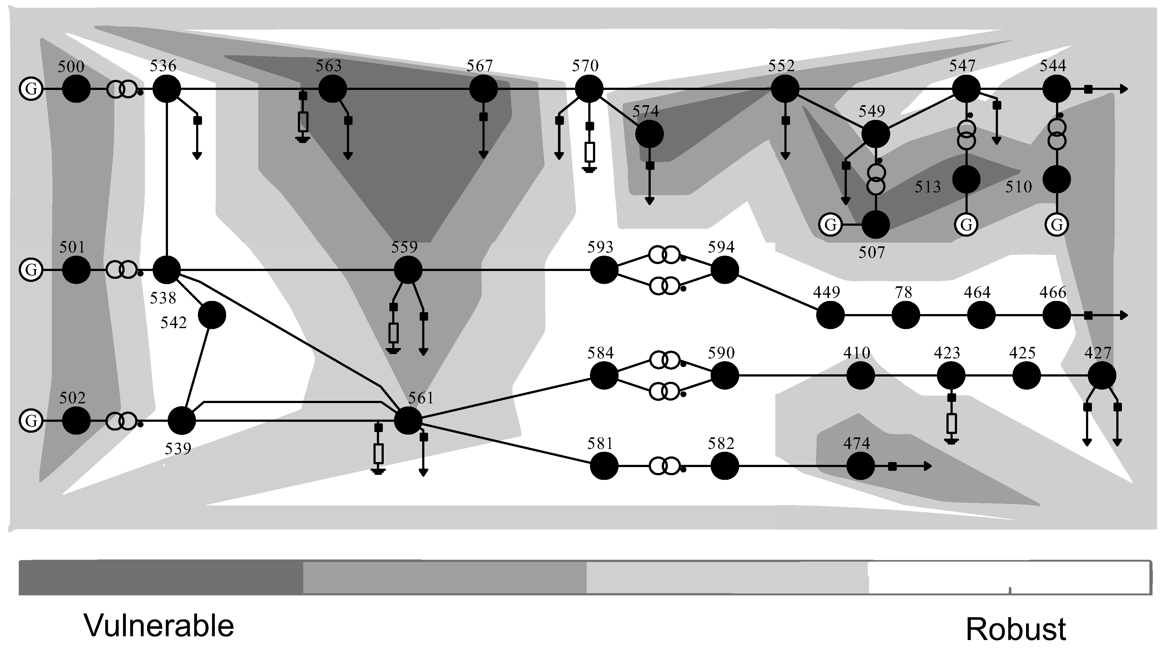
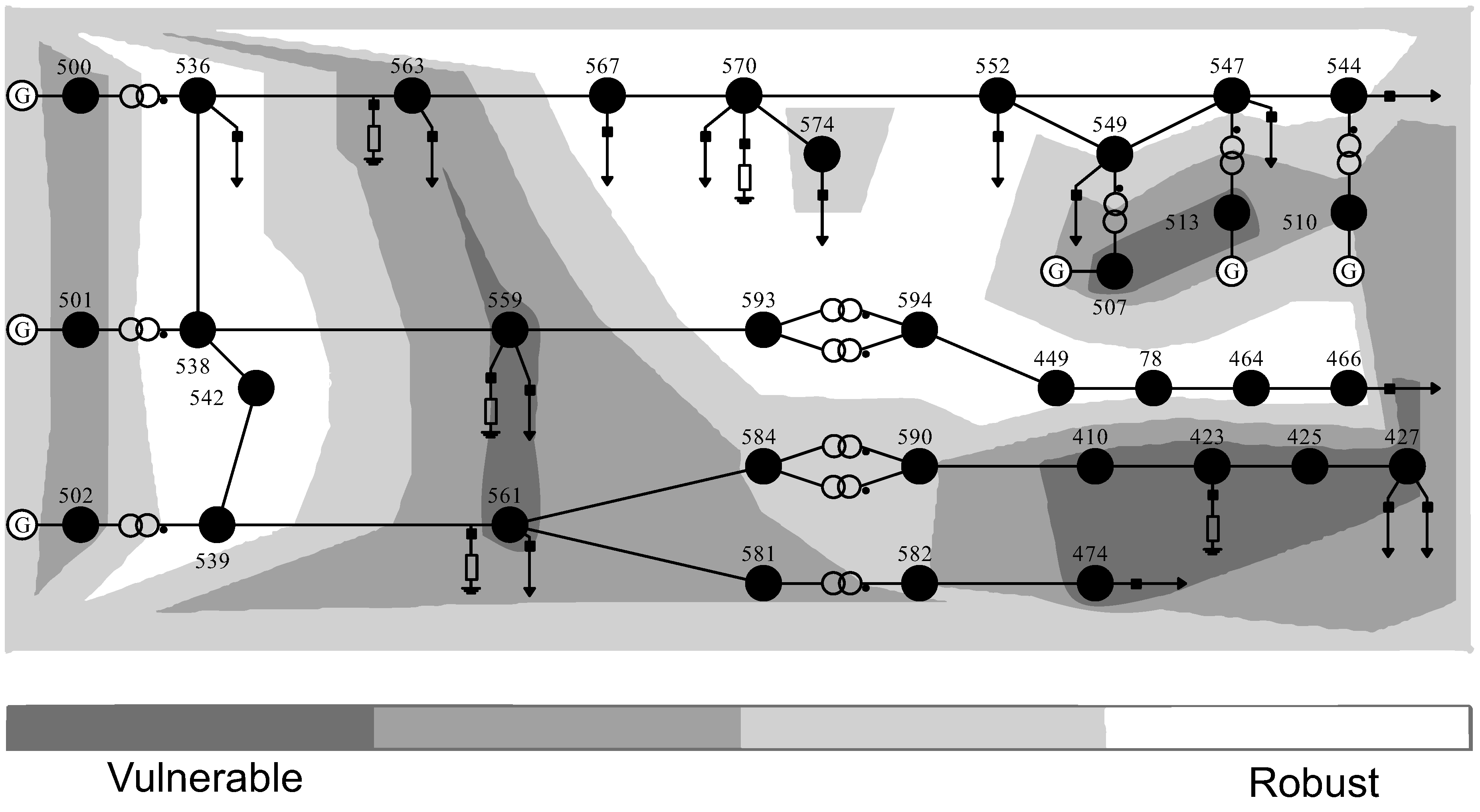
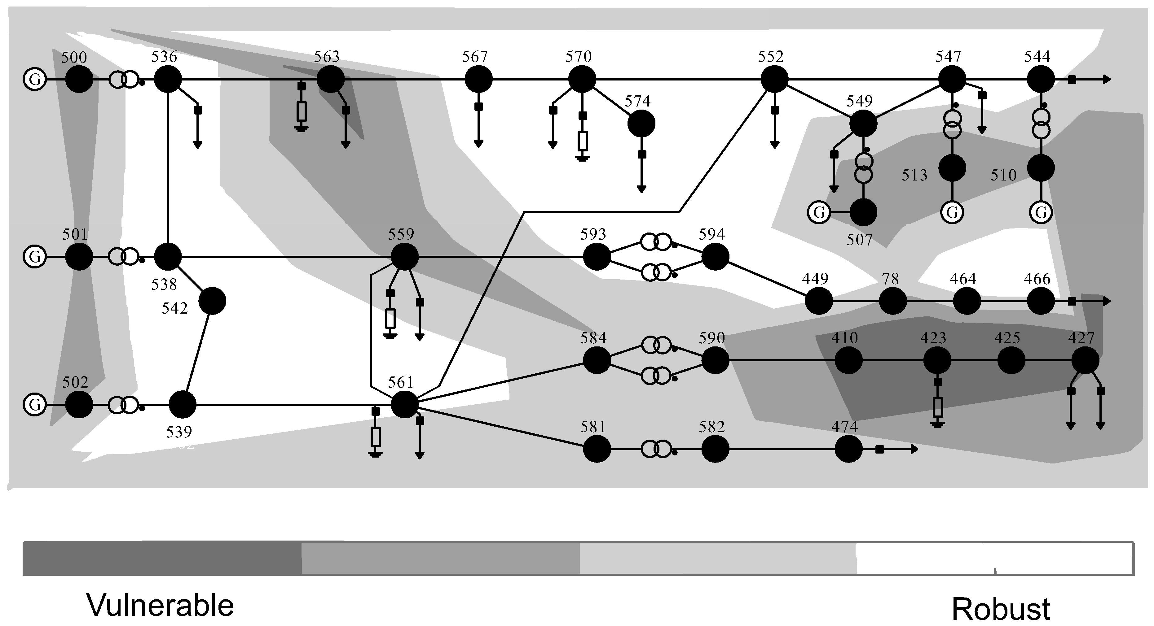
• Group the buses into areas, according to their robustness level. It is possible to generate an diagram where buses are shaded according to their vulnerability level and the RAs are formed.
• Propose a new guideline for reconnection by linking two buses according to their robustness levels. The vulnerability level defines the first connection. Then, the vulnerability profile is calculated for the new operating point. The process is then repeated, so a new connection is proposed based on the updated vulnerability levels.
• Compare statically and dynamically the proposed guidelines with the standard one adopted by the ISO. In addition, voltage stability analysis is considered as a robustness criterion for the guidelines.

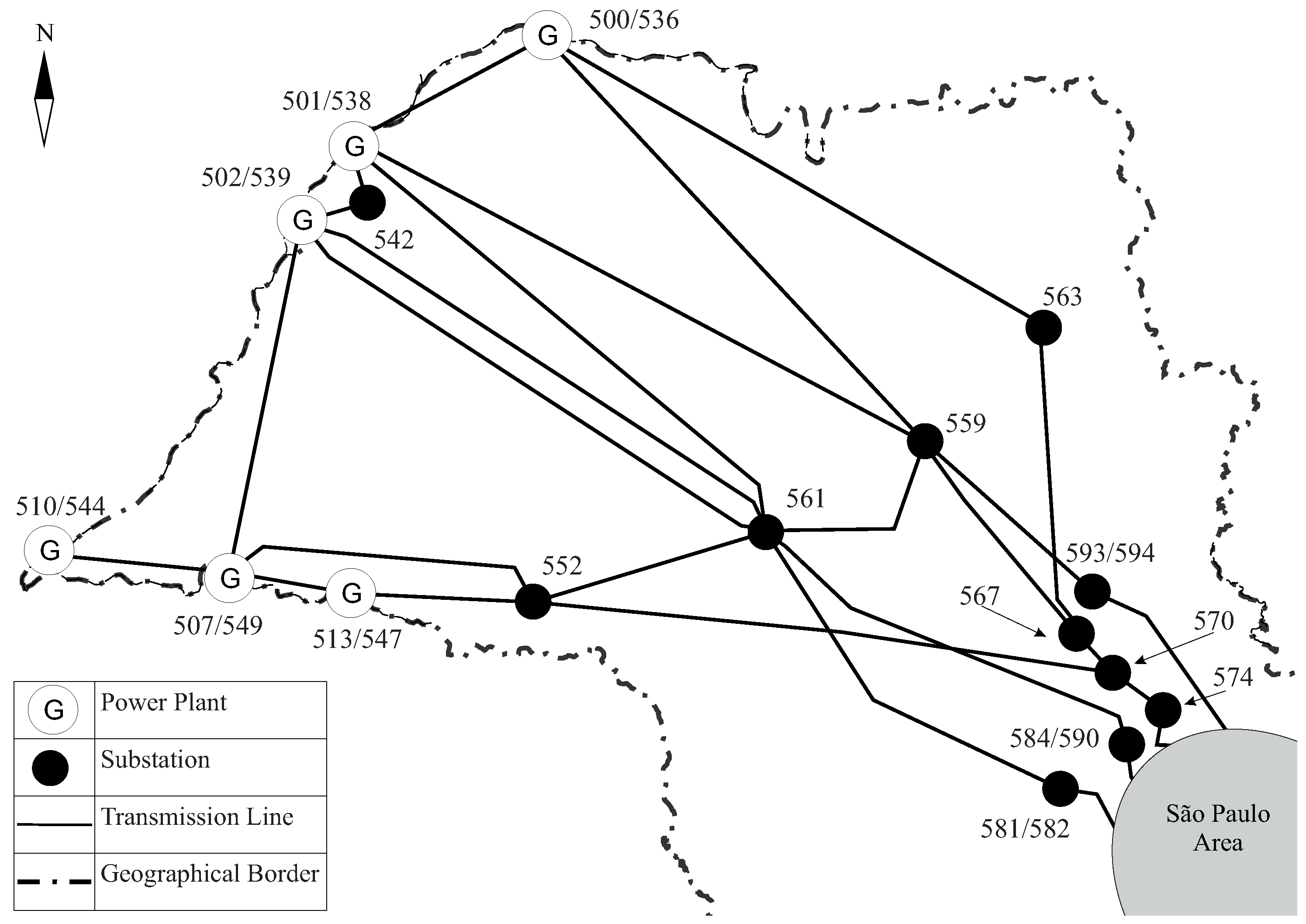
3.2. Real Case Study System

The real case power system selected is a part of the São Paulo State power system in Brazil, which has a 440 kV bulk connected to 345 kV and 230 kV branches and local loads as in Figure 3, covering 248,209 km².

The system presents five restoration areas, known as corridors, due to their long length characteristics. Each corridor is able to restore independently and form a small electric island, which is later connected to the grid, under the ISO supervision. Corridors are identified by the main hydropower plant presented in each one: 500 (Água Vermelha), 501 (Ilha Solteira), 502 (Jupiá), 507 (Capivara), and 510 (Porto Primavera). The converged power flow case for this system is presented in

Table A1. Base case power flow and the Robustness Area (RA) calculation.

Bus	V	θ	${\mathit{P}}_{\mathit{g}}$	${\mathit{Q}}_{\mathit{g}}$	${\mathit{P}}_{\mathit{l}}$	${\mathit{Q}}_{\mathit{l}}$	${\mathit{E}}_{\mathit{p}}$
78	0.920	−22.3	-	-	-	-	91.0
410	1.000	−24.0	-	-	-	-	4.8
423	0.986	−25.5	-	-	-	-	−7.3
425	0.983	−26.1	-	-	-	-	0.9
427	0.978	−27.3	-	-	250.0	85.4	11.0
449	0.923	−21.5	-	-	-	-	142.3
464	0.916	−23.3	-	-	-	-	280.4
466	0.915	−23.4	-	-	160.0	35.3	244.0
474	1.041	−18.0	-	-	30.0	10.4	11.3
500	0.960	−0.6	306.3	−99.5	-	-	33.9
501	0.930	0.0	495.1	−342.1	-	-	40.4
502	1.000	−2.0	364.8	5.9	-	-	29.3
507	0.995	12.2	175.0	−49.7	-	-	18.3
510	1.000	16.0	394.7	−111.9	-	-	37.8
513	0.990	13.9	150.0	−70.4	-	-	14.2
536	0.975	−3.1	-	-	120.0	48.6	46,905.3
538	0.972	−3.4	-	-	-	-	45,395.4
539	1.001	−5.4	-	-	150.0	60.0	96.6
542	0.989	−4.5	-	-	-	-	115.3
544	1.017	12.9	-	-	9.0	3.7	91.7
547	1.017	10.8	-	-	65.0	28.6	129.4
549	1.010	9.4	-	-	100.0	38.4	89.6
552	1.002	6.5	-	-	65.0	23.5	50,075.2
559	0.912	−15.5	-	-	150.0	50.4	14.8
561	1.042	−16.8	-	-	120.0	45.0	16.2
563	0.952	−8.8	-	-	130.0	54.1	22.3
567	0.947	−9.5	-	-	180.0	79.2	140.0
570	0.947	−9.1	-	-	160.0	39.1	44,504.9
574	0.941	−9.9	-	-	160.0	73.6	53.5
581	1.038	−17.6	-	-	-	-	42.0
582	1.040	−17.7	-	-	-	-	48.6
584	1.015	−21.9	-	-	-	-	49.2
590	1.012	−22.5	-	-	-	-	51.1
593	0.924	−20.7	-	-	-	-	119.3
594	0.924	−21.1	-	-	-	-	200.2

located in Appendix A, where bus voltage magnitude (V), voltage angle (θ), generated power ($S_g=P_g+j{Q}_g$), load power ($S_l=P_l+j{Q}_l$), and the robustness level ($E_p$) are indicated.

The restoration guidelines adopted by the ISO are available online [4,5] along with the system data [35] so that experiments related to the Brazilian power system can be reproduced. Background studies regarding the Brazilian PSR are also available [4,5], including the step-by-step report to perform the system restoration. Among the background studies offered by the ISO, there are important ones simulated in this paper, such as: the load estimation, voltage control, Standing Phase Angle (SPA), load ramping and frequency control.

The long high voltage transmission lines used to restore this system are a key feature, leading to problems in maintaining the reactive power balance. As a consequence, buses and transmission lines are equipped with shunt reactors to perform reactive power control. Since buses are not uniformly distributed along the state area, a representative diagram is presented in Figure 4, with the RA mapping as the background.

3.3. Establishing a New Guideline for Restoration Procedure

The base case scenario, presented in Figure 4, is the schematic diagram of the studied power system using the result of each bus robustness level $E_p$ as background. The $E_p$ is presented in Table A1 in the right-hand side column.

Figure 4 depicts the first step of the CP [4,5] during the restoration plan for the São Paulo State grid, where the five restoration areas are synchronized. After the synchronization, the ISO sets the power plant at bus 501 as the slack bus [4,5]. Bus 501 is also responsible for the secondary frequency control. The ISO determines that, at this moment of the restoration, two transmission lines are connected: 538 to 561 and the second transmission line from 539 to 561. If both transmission lines are successfully connected, a maximum of 100 MW load is reconnected at bus 561. The robustness area diagram for the ISO proposed scenario is presented in Figure 5. According to the RA analysis, the restoration plan proposed by the ISO has a positive impact on the bus 502 corridor, improving the robustness level significantly, and also a negative effect on the strength level of buses 500, 507 and 510 restoration corridors.

It is worth noting that generation buses are located in vulnerable areas, as depicted in Figure 4. This situation has also been observed in different power systems, when these are operating in low load profile. As a consequence of the low load profile, generators are responsible to consume a large amount of the reactive power generated by the transmission lines. This phenomena is captured by the RA tool and translated in the form of a vulnerable area.

Since the ISO proposes two transmission lines to be reconnected before the load pick-up at bus 561, the proposed restoration guideline also considers two transmission lines to be reconnected before the load pick-up. From the base case scenario, one can see in Figure 4 that the bus 561, which is responsible for restoring a load amount of 100 MW, is in a vulnerable area. Hence, possible restoration scenarios were tested regarding SPA, generation limits, voltage level limits, transmission lines, transformer capacity, and the system’s RA.

From all of the scenarios tested, the selected one addresses two main issues: the robustness level of bus 561 and the robustness level of the system as a whole. The robustness level of bus 561 is important because it is the bus to pick-up a load amount of 100 MW. The whole system robustness level is also taken into consideration because the experience has shown that systems in which the robustness level differences are mitigated tend to present improved voltage stability. This is because systems with balanced robustness level can locally supply more reactive power than unbalanced systems.

Considering the aforementioned requirements, the proposed scenario is depicted in Figure 6, where the two transmission lines to be reconnected before the load pick-up in bus 561 takes place are 539 to 561, and the second transmission line from 552 to 561. The proposed guideline not only improves the robustness level of bus 561 but also benefits the robustness level of the whole system.

Aiming to compare both solutions, a number of studies are prepared, dividing into two main categories: voltage stability and dynamic stability. The voltage stability assessment is presented in Section 4.1, where load flow limits are checked. Reactive power margin and SPA analysis are also considered. Section 4.2 presents time domain simulation analyzing the system under a load shedding, a severe and realistic event during PSR.

4. Stability Assessments

4.1. Voltage Stability Assessment

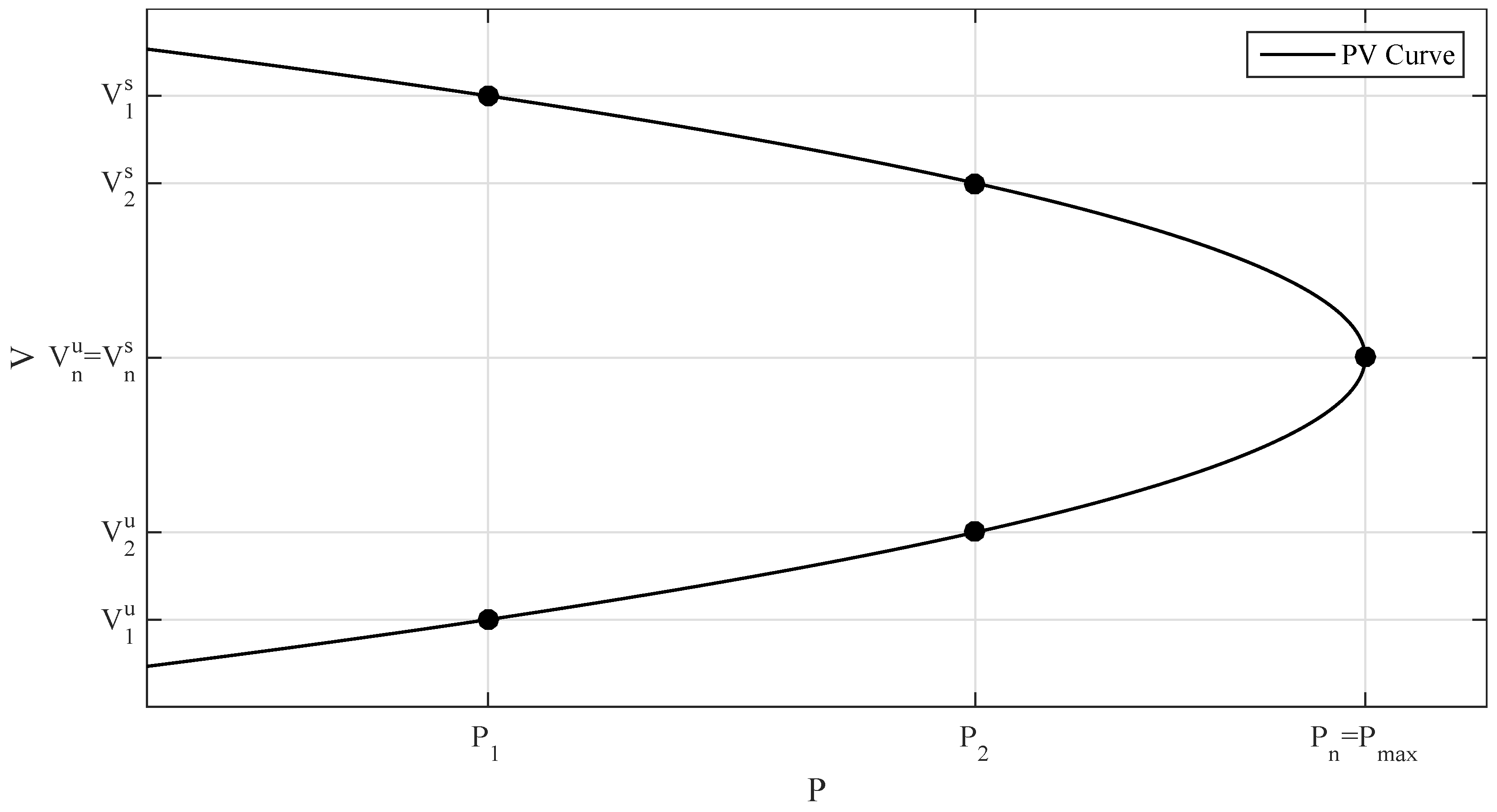
4.1.1. PV Curve Analysis

The first topic of analysis is the load margin, defined as the difference between the maximum loading point $P_{\max }$ and the load associated with the operation point. Note that voltage stability studies are meant to determine the load that a system may sustain in a stable manner. Thus, it is not expected to carry out such studies in a black start scenario. However, this may be useful as a robustness index, since the areas formed along the process may sustain a load increase in better conditions. This is important for black start conditions, since the system loading is gradually increased.

Considering the same system parameters and the same initial load, the configuration defined by the ISO can sustain 27% of additional load, whereas the topology obtained by the methodology proposed here can reach up to 32%. This first result shows that the proposed guideline renders a safer position if compared with the ISO approach and an increased transmission capacity.

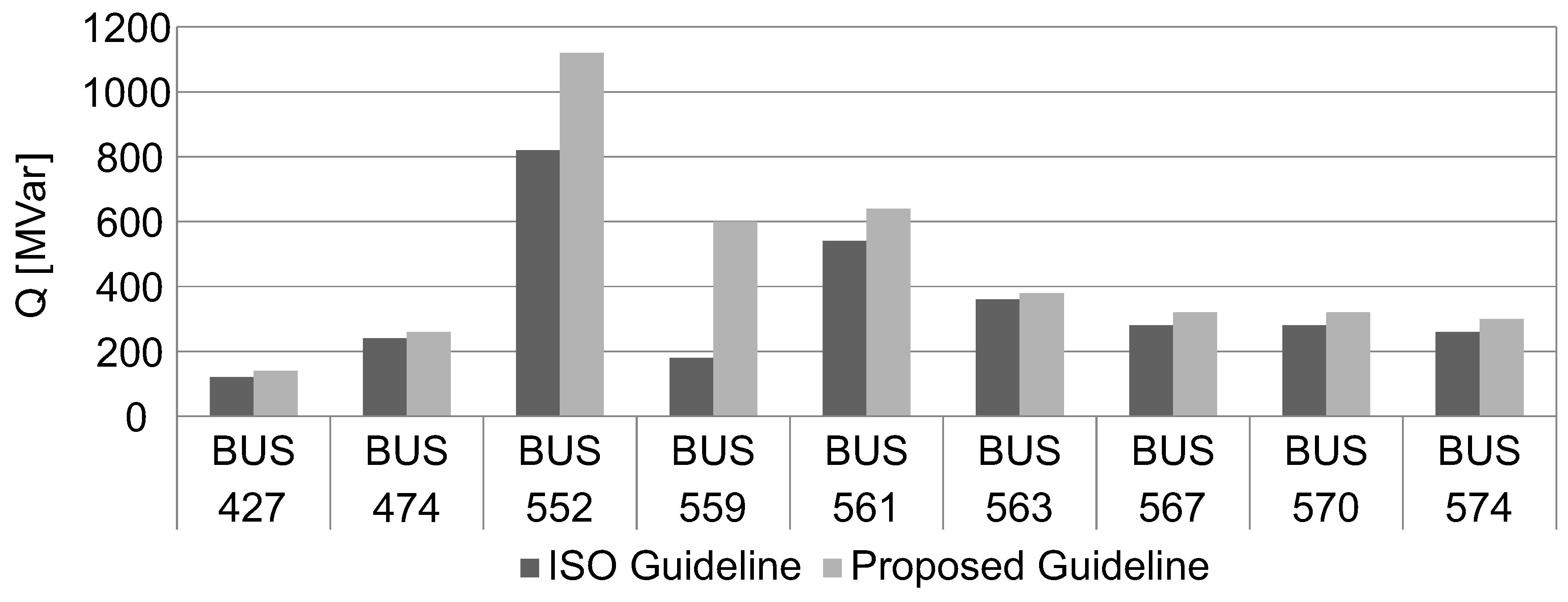
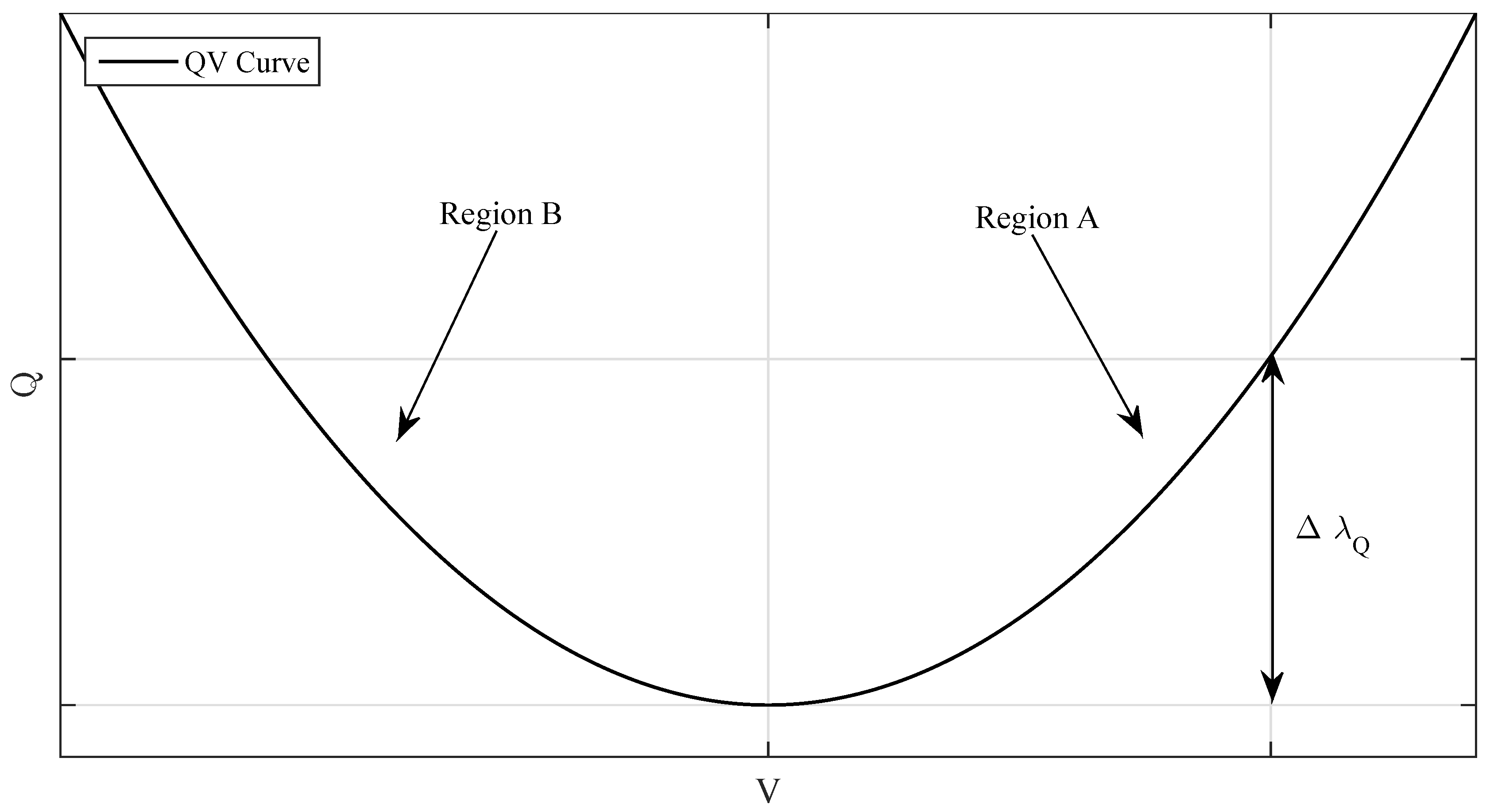
4.1.2. QV Curve Analysis

The second comparison relates to the reactive power load margin yielded by the QV curve, which measures the capability of each bus in providing reactive power. The calculation of this voltage stability index is obtained by increasing the reactive power only in the bus of interest until the system reaches the voltage collapse. The proposed guideline provides a larger reactive power load margin for the majority of the buses considered, as shown in Figure 7. Bearing in mind that voltage stability issues are strongly associated with reactive power availability [36], the proposed solution presents a well-conditioned transmission network, which is able to supply all system loads with a security margin considerably higher than the proposed standard solution.

4.1.3. Standing Phase Angle Analysis

When a transmission line is to be connected, it faces an SPA, defined by the difference between the voltage angles at both ends of the transmission line. Connecting a transmission line with a large SPA impacts switchers, reduces generator shaft life-cycles and can lead to dynamic instability [37]. Due to this, the module of this SPA is monitored, as shown in

Table 1. Standing Phase Angles (SPAs) in the module for the transmission lines closed in each restoration plan.

	Transmission Line		Standing Phase
	From	To	Angle [°]
Proposed Guideline	552	561	0.8
	559	561	3.1
ISO Guideline	539	561	7.8
	538	561	3.9

.

The SPA obtained through the proposed methodology is smaller than the one calculated under the guideline proposed by the ISO for all loop closures considered. This SPA has a direct impact on the power transmitted through the transmission line at the instant that the switch is closed. Such a value is a metric during the restoration planning; therefore, it is limited by the ISO. Considering the results from the voltage stability assessment, it is possible to conclude that the methodology proposed here can provide accurate information to perform the restoration procedure.

4.2. Dynamic Stability Assessment

Complementing the voltage stability analysis, dynamic stability assessment provides time domain responses for events of interest during the restoration procedure. Considering the SPAs presented in Table 1 as the initial conditions, electromechanic surges caused by the reconnections are assessed. Simulations are performed considering a 20 s horizon with a fixed step of 3 ms. The IEEE 7th order model has been employed to model the synchronous machines:

$$\begin{array}{ccc}\hfill \dot{\delta }& =& \omega -{\omega }_s,\hfill \end{array}$$

(6)

$$\begin{array}{ccc}\hfill \dot{\omega }& =& \frac{1}{2H}\left[T_m-\left(E_q^{\prime }-X_d{I}_d\right)I_q-\left(E_d^{\prime }+X_q{I}_q\right)I_d-D\left(\omega -{\omega }_s\right)\right],\hfill \end{array}$$

(7)

$$\begin{array}{ccc}\hfill {\dot{E}}_q^{\prime }& =& \frac{1}{T_{d0}^{\prime }}\left[-E_q^{\prime }-\left(X_d-X_d^{\prime }\right)I_d+E_{fd}\right],\hfill \end{array}$$

(8)

$$\begin{array}{ccc}\hfill {\dot{E}}_d^{\prime }& =& \frac{1}{T_{q0}^{\prime }}\left[-E_d^{\prime }+\left(X_q-X_q^{\prime }\right)I_q\right],\hfill \end{array}$$

(9)

$$\begin{array}{ccc}\hfill {\dot{E}}_{fd}& =& \frac{1}{T_E}\left[-K_E{E}_{fd}-S_E\left(E_{fd}\right)+V_r\right],\hfill \end{array}$$

(10)

$$\begin{array}{ccc}\hfill {\dot{V}}_r& =& \frac{1}{T_A}\left[-V_r+K_A\left(V_{ref}-V-V_s\right)\right],\hfill \end{array}$$

(11)

$$\begin{array}{ccc}\hfill {\dot{V}}_s& =& \frac{1}{T_F}\left[-V_s+\frac{K_F}{T_E}\left(-K_e{E}_{fd}+V_R-S_e\left(E_{fd}\right)\right)\right].\hfill \end{array}$$

(12)

It is a complete model including voltage regulator $V_r$ power system stabilizer $V_s$, and saturation $S_E\left(E_{fd}\right)$. For more details, please refer to [38]. The direct and quadrature axis current are calculated by:

$$\begin{array}{ccc}\hfill I_d& =& \frac{E_q^{\prime }-Vcos\left(\delta -\theta \right)}{X_d^{\prime }},\hfill \end{array}$$

(13)

$$\begin{array}{ccc}\hfill I_q& =& \frac{Vsin\left(\delta -\theta \right)-E_d^{\prime }}{X_q^{\prime }}.\hfill \end{array}$$

(14)

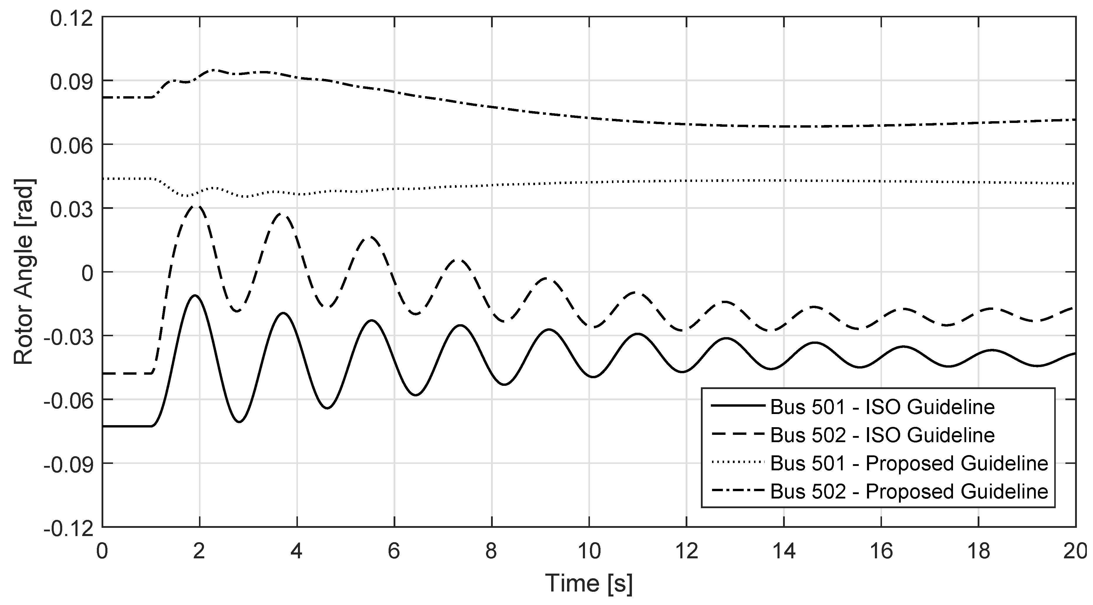
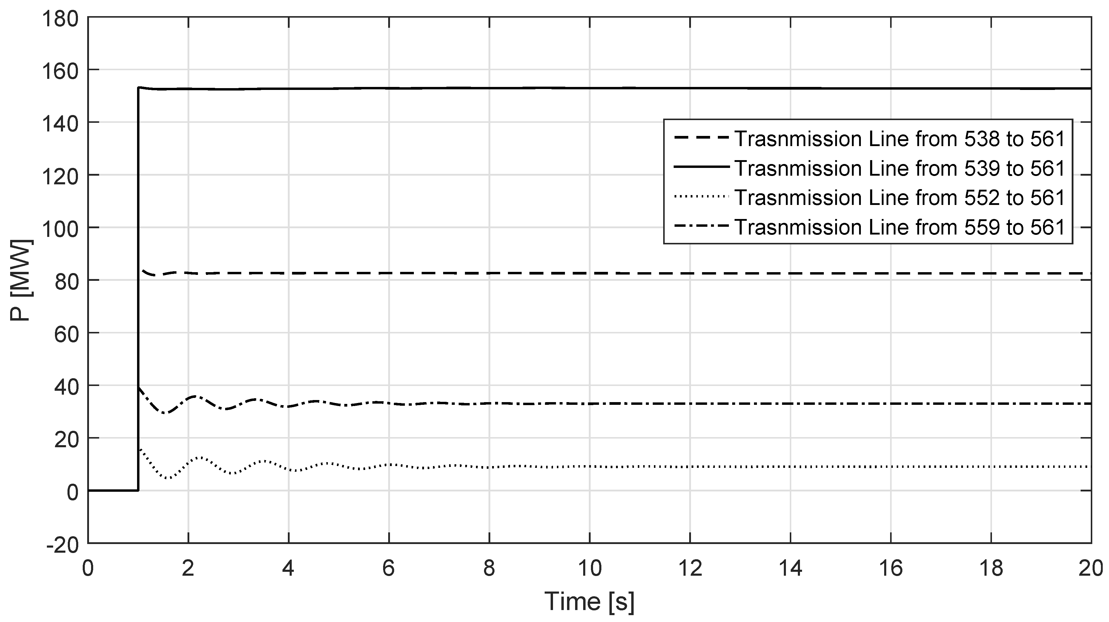
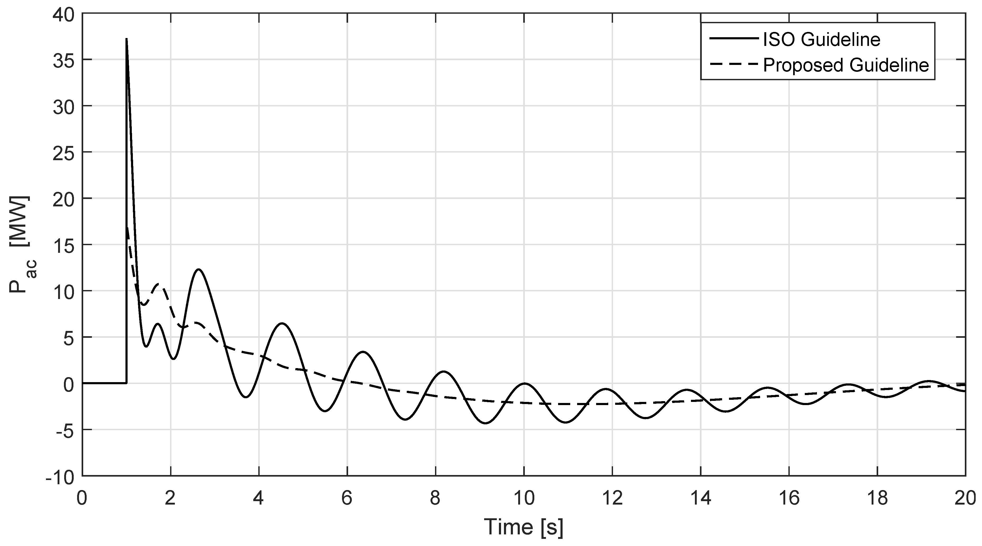
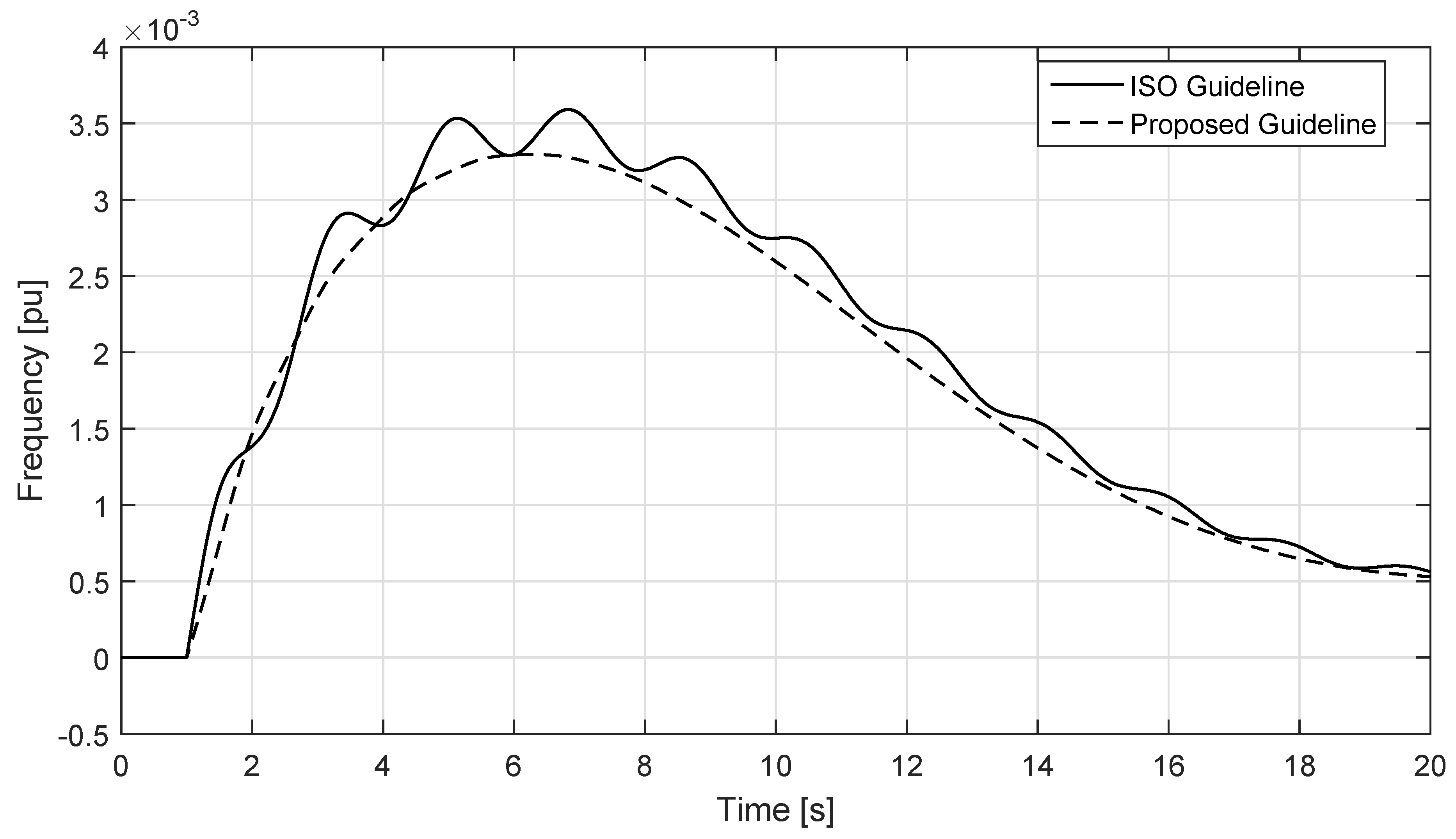
4.2.1. Loop Closure Simulation

The simulation results are shown in Figure 8, which shows the active power flowing in the connected transmission lines. Note that the methodology proposed in this paper yields a smaller active power flow in transient and steady-state conditions, rendering this technique more effective for this purpose, since lower impacts are observed. In the sequence, another dynamic event is considered. Under normal system operation, short-circuits are considered the main source of disturbance in dynamic stability study. In restoration study, short-circuits are rarely considered, since it is more realistic to consider load pick-ups, load shedding, and tripping off transmission lines.

4.2.2. Load Shedding Simulation

The event considered is a full load shedding at bus 561, which is a severe event and is likely to occur to recently connected loads during Power System Restoration (PSR) due to inappropriate protective actions during grid instabilities [11]—for instance: voltage sags or sudden load variations. The results obtained from both solutions are transient stable and dynamic stable, as demonstrated by the rotor angle in relation to the system mass center, depicted in Figure 9. The proposed solution, however, presents smoother behaviour and smaller angular deviation in relation to the ISO guideline solution, indicating that the angular stability is improved.

At the instant of the load shedding, there is an abrupt reduction in the total electric power consumption, and, until the governor control acts, there is more mechanical power being injected in the machine than electric power being delivered to the grid. This power mismatch is called accelerating power and is calculated by $P_{ac}=P_m-P_e$; its behaviour is depicted in Figure 10 for both methodologies. The ISO approach yields an oscillatory response and a settling time of 18 s is observed for both methodologies.

Two main differences are shown for the $P_{ac}$ response: maximum peak and oscillatory response. The maximum peak after the event is 37 MW for the ISO guideline, whereas, under the methodology proposed using the RA tool, the initial $P_{ac}$ is 17 MW. Sudden power mismatch of the generator unities induces torque variation on the generator-turbine shaft, reducing its life-cycle. Consequently, solutions that present smaller power variations are preferable, as the proposed guideline for this scenario. The second divergence between the two guidelines is the oscillatory response presented by the ISO guideline leading to angle excursions and torque variations.

The effect of the $P_{ac}$ in the system frequency is shown in Figure 11, where the frequency deviation response shows the smooth behaviour and slightly smaller transient deviation presented by the proposed guideline. As a consequence of the $P_{ac}$, the system frequency increases from 1 s to 6 s, when $P_m>P_e$, and after 18 s, the simulation shows the frequency reaches a new level, caused by the droop speed regulators used on governor power plants. This kind of control allows the power mismatch to be shared by power plants, according to their characteristics and capacity. Thus, it cannot neutralize the steady state frequency deviation completely. There are regulators, based on integration control, to restore the system frequency to the rated value; however, these rely on slow response, and the simulation horizon is too short to capture this dynamical response. Additionally, the automatic secondary speed regulation is not considered during full restoration procedure, and the long-term frequency control is manually performed. The smooth behaviour of the proposed guideline, however, is clearly observed in Figure 11.

5. Conclusions

PSR procedures are among the most complex operations faced by system operators. The Brazilian ISO divides this procedure into two stages. First, the FP is dedicated to create corridors of load in order to start the machines. The second stage is the CP that consists of connecting the islands formed during the first stage. This paper proposed a new guideline to deal with the second stage. For this purpose, a system robustness based-method is applied. The new configuration is tested under static and dynamic analyses, and compared to the guidelines adopted by the ISO.

As for the static studies, active power margin and reactive power margin are used to investigate the impact that the RA tool has on the system ability in supply load increments. The results obtained show larger active power load margin for the system as a whole and an enhanced reactive power margin for the buses monitored.

The dynamic implications are studied by time domain simulations following the switching of the transmission lines; thus, the transient response is monitored. A full load shedding is also tested, and the proposed guideline presented smoother behaviour in comparison with the response provided by the ISO guideline.

The tests carried out in a part of the Brazilian system show that the RA tool can be used as a helper for PSR planning. Such ability is demonstrated by comparing a proposed guideline to the one currently employed by the ISO. In fact, by using the RA tool, one can re-evaluate standard guidelines and propose more stable alternatives for PSR.

References

1. Adibi, M.; Martins, N.; Watanabe, E. The impacts of FACTS and other new technologies on power system restoration dynamics. In Proceedings of the 2010 IEEE Power and Energy Society General Meeting, Providence, RI, USA, 25–29 July 2010; pp. 1–6.
2. Allen, E.; Stuart, R.; Wiedman, T. No light in August: Power system restoration following the 2003 North American Blackout. IEEE Power Energy Mag. 2014, 12, 24–33. [Google Scholar] [CrossRef]
3. Bernardon, D.; Sperandio, M.; Garcia, V.; Canha, L.; da Rosa Abaide, A.; Daza, E. AHP Decision-Making algorithm to allocate remotely controlled switches in distribution networks. IEEE Trans. Power Deliv. 2011, 26, 1884–1892. [Google Scholar] [CrossRef]
4. Brazilian Independent System Operator. Networks Proceedings 21.6 — System Restoration Studies, 2009; Brazilian Independent System Operator: Rio de Janeiro, Brazil, 2016. (In Portuguese) [Google Scholar]
5. Brazilian Independent System Operator. Networks Proceedings 10.11 — Network Restoration after Disturbances, 2010; Brazilian Independent System Operator: Rio de Janeiro, Brazil, 2016. (In Portuguese) [Google Scholar]
6. Gomes, P.; de Lima, A.; de Padua Guarini, A. Guidelines for power system restoration in the Brazilian system. IEEE Trans. Power Syst. 2004, 19, 1159–1164. [Google Scholar] [CrossRef]
7. Camillo, M.; Romero, M.; Fanucchi, R.; de Lima, T.; Marques, L.; Delbem, A.; London, J. Validation of a methodology for service restoration on a real Brazilian distribution system. In Proceedings of the 2014 IEEE PES Transmission Distribution Conference and Exposition—Latin America (PES T D-LA), Medellin, Colombia, 9–13 September 2014; pp. 1–6.
8. Decker, I.; Agostini, M.; e Silva, A.; Dotta, D. Monitoring of a large scale event in the Brazilian power system by WAMS. In Proceedings of the 2010 iREP Symposium on Bulk Power System Dynamics and Control (iREP)—VIII (iREP), Rio de Janeiro, Brazil, 1–6 August 2010; pp. 1–8.
9. Electric Energy National Agengy ANEEL. Fiscalization report on the 10th of November 2009 Blackout in Brazil, 2010; Electric Energy National Agengy ANEEL: Brasilia, Brazil, 2010. (In Portuguese) [Google Scholar]
10. Mota, A.; Mota, L.; Morelato, A. Visualization of Power System Restoration Plans Using CPM/PERT Graphs. IEEE Trans. Power Syst. 2007, 22, 1322–1329. [Google Scholar] [CrossRef]
11. Adibi, M. Power system restoration the second task force report. In Power System Restoration: Methodologies and Implementation Strategies; Wiley-IEEE Press: Hoboken, NJ, USA, 2000; pp. 10–16. [Google Scholar]
12. Yari, V.; Nourizadeh, S.; Ranjbar, A. Wide-Area frequency control during power system restoration. In Proceedings of the 2010 IEEE Electric Power and Energy Conference (EPEC), Halifax, NS, Canada, 25–27 August 2010; pp. 1–4.
13. Silva, B.; Moreira, C.; Seca, L.; Phulpin, Y.; Peças Lopes, J. Provision of inertial and primary frequency control services using offshore multiterminal HVDC networks. IEEE Trans. Sustain. Energy 2012, 3, 800–808. [Google Scholar] [CrossRef]
14. Yari, V.; Nourizadeh, S.; Ranjbar, A. Determining the best sequence of load pickup during power system restoration. In Proceedings of the 2010 9th International Conference on Environment and Electrical Engineering (EEEIC), Prague, Czech Republic, 16–19 May 2010; pp. 1–4.
15. Nourizadeh, S.; Karimi, M.; Ranjbar, A.; Shirani, A. Power system stability assessment during restoration based on a wide area measurement system. Gener. Transm. Distrib. IET 2012, 6, 1171–1179. [Google Scholar] [CrossRef]
16. Duffey, R.; Ha, T. The probability and timing of power system restoration. IEEE Trans. Power Syst. 2013, 28, 3–9. [Google Scholar] [CrossRef]
17. Ren, F.; Zhang, M.; Soetanto, D.; Su, X. Conceptual design of a multi-agent system for interconnected power systems restoration. IEEE Trans. Power Syst. 2012, 27, 732–740. [Google Scholar] [CrossRef]
18. Sun, W.; Liu, C.C.; Zhang, L. Optimal generator start-up strategy for bulk power system restoration. IEEE Trans. Power Syst. 2011, 26, 1357–1366. [Google Scholar] [CrossRef]
19. Wang, C.; Vittal, V.; Sun, K. OBDD-Based sectionalizing strategies for parallel power system restoration. IEEE Trans. Power Syst. 2011, 26, 1426–1433. [Google Scholar] [CrossRef]
20. Shi, L.; Ding, H.; Xu, Z. Determination of weight coefficient for power system restoration. IEEE Trans. Power Syst. 2012, 27, 1140–1141. [Google Scholar] [CrossRef]
21. Lin, Z.; Wen, F. Discussion on “Optimal generator start-up strategy for bulk power system restoration”. IEEE Trans. Power Syst. 2011, 27, 1357–1366. [Google Scholar] [CrossRef]
22. Oliveira, D.; Zambroni de Souza, A.; Almeida, A.; Lima, I. An artificial immune approach for service restoration in smart distribution systems. In Proceedings of the 2015 IEEE PES, Innovative Smart Grid Technologies Latin America (ISGT LATAM), Montevideo, Uruguay, 5–7 October 2015; pp. 1–6.
23. Siqueira, D.; Alberto, L.; Bretas, N. Generalized energy functions for a class of lossy networking preserving power system models. In Proceedings of the 2015 IEEE International Symposium on Circuits and Systems (ISCAS), Lisbon, Portugal, 24–27 May 2015; pp. 926–929.
24. Kumar, A.; Bhagat, S. Voltage stability analysis using lyapunov energy function. In Proceedings of the 2015 1st Conference on Power, Dielectric and Energy Management at NERIST (ICPDEN), Itanagar, India, 10–11 January 2015; pp. 1–6.
25. Marujo, D.; Zambroni de Souza, A.; Prada, R. On reverse operating conditions identification. In Proceedings of the 2015 IEEE Eindhoven PowerTech, Eindhoven, The Netherlands, 29 June–2 July 2015; pp. 1–6.
26. Kundur, P. Power System Stability and Control; McGraw-Hill: New York, NY, USA, 1994. [Google Scholar]
27. Marujo, D.; Zambroni de Souza, A.; Lima Lopes, B.; Santos, M.; Lo, K. On control actions effects by using QV curves. IEEE Trans. Power Syst. 2015, 30, 1298–1305. [Google Scholar] [CrossRef]
28. Van Cutsem, T.; Vournas, C. Voltage Stability of Electric Power Systems; Springer: New York, NY, USA, 2008. [Google Scholar]
29. De Lorenci, E.V.; de Souza, A.C.Z. Energy function applied to voltage stability studies—Discussion on low voltage solutions with the help of tangent vector. Electr. Power Syst. Res. 2016, 141, 290–299. [Google Scholar] [CrossRef]
30. de Souza, A.Z.; Leme, R.C.; Vasconcelos, L.F.B.; Lopes, B.I.L.; da Silva Ribeiro, Y.C. Energy function and unstable solutions by the means of an augmented Jacobian. Appl. Math. Comput. 2008, 206, 154–163. [Google Scholar]
31. Overbye, T. Use of energy methods for on-line assessment of power system voltage security. IEEE Trans. Power Syst. 1993, 8, 452–458. [Google Scholar] [CrossRef]
32. Iba, K.; Suzuki, H.; Egawa, M.; Watanabe, T. A method for finding a pair of multiple load flow solutions in bulk power systems. IEEE Trans. Power Syst. 1990, 5, 582–591. [Google Scholar] [CrossRef]
33. Klump, R.; Overbye, T. A new method for finding low-voltage power flow solutions. In Proceedings of the 2000 IEEE Power Engineering Society Summer Meeting, College Station, TX, USA, 16–20 July 2000; Volume 1, pp. 593–597.
34. De Souza, A.Z. Tangent vector applied to voltage collapse and loss sensitivity studies. Electr. Power Syst. Res. 1998, 47, 65–70. [Google Scholar] [CrossRef]
35. Brazilian Independent System Operator. Brazilian System Technical Data; Brazilian Independent System Operator: Rio de Janeiro, Brazil. (In Portuguese)
36. Mohn, F.; de Souza, A. Tracing PV and QV curves with the help of a CRIC continuation method. IEEE Trans. Power Syst. 2006, 21, 1115–1122. [Google Scholar] [CrossRef]
37. Martins, N.; de Oliveira, E.; Pereira, J.; Ferreira, L. Reducing Standing Phase Angles via Interior Point Optimum Power Flow for Improved System Restoration. In Proceedings of the 2004 IEEE PES Power Systems Conference and Exposition, New York, NY, USA, 10–13 October 2004; Volume 1, pp. 404–408.
38. Anderson, P.; Fouad, A. Power System Control and Stability, 2nd ed.; Wiley India Pvt. Limited: Delhi, India, 2008. [Google Scholar]
Figure 1. Regions of operation in a QV curve.
Energies 10 00099 g001
Figure 2. The PV curve.
Energies 10 00099 g002
Figure 3. Geographical representation of the São Paulo State power grid. The highlighted area represents the state’s capital city.
Energies 10 00099 g003
Figure 4. Robustness Areas (RA) map for the São Paulo State power grid during restoration—base case scenario.
Energies 10 00099 g004
Figure 5. RA map for São Paulo State power grid during restoration — Independent System Operator (ISO) guidelines.
Energies 10 00099 g005
Figure 6. Robustness areas (RA) map for the São Paulo State power grid during restoration—proposed plan.
Energies 10 00099 g006
Figure 7. Reactive power margin for selected load buses.
Energies 10 00099 g007
Figure 8. Transmitted active power through the connected transmission line.
Energies 10 00099 g008
Figure 9. Power plant rotor angle in relation to the system mass center.
Energies 10 00099 g009
Figure 10. Accelerating power response for the power plant at bus 501.
Energies 10 00099 g010
Figure 11. Frequency deviation response for the power plant at bus 501.
Energies 10 00099 g011