A Scatter Search Heuristic for the Optimal Location, Sizing and Contract Pricing of Distributed Generation in Electric Distribution Systems

Abstract

In this paper we present a scatter search (SS) heuristic for the optimal location, sizing and contract pricing of distributed generation (DG) in electric distribution systems. The proposed optimization approach considers the interaction of two agents: (i) the potential investor and owner of the DG, and (ii) the Distribution Company (DisCo) in charge of the operation of the network. The DG owner seeks to maximize his profits from selling energy to the DisCo, while the DisCo aims at minimizing the cost of serving the network demand, while meeting network constraints. To serve the expected demand the DisCo is able to purchase energy, through long-term bilateral contracts, from the wholesale electricity market and from the DG units within the network. The interaction of both agents leads to a bilevel programming problem that we solve through a SS heuristic. Computational experiments show that SS outperforms a genetic algorithm hybridized with local search both in terms of solution quality and computational time.

1. Introduction

Distributed generation (DG), known as the small-scale production of electricity near consumers, has become increasingly common in distribution networks in the last decade. This trend has been driven by different factors. Such as environmental concerns, fossil fuel resource depletion, and new advances in small-scale generation technologies [1]. Distribution systems were not originally designed to operate with DG; therefore, its insertion in the network must be carefully planned out. In this regard, the integration of DG in distribution networks has been the focus of several studies [2,3,4,5,6,7,8,9,10,11,12]. Most of these studies aim at harvesting the potential benefits of DG such as: reduction of power losses [2,3,4], improvement of voltage profile [5], improvement of stability [6], and deferral of investments [7]. In recent years there has been an important increase in the participation of DG in distribution systems. This has been motivated by several factors that include new advances in microgeneration and storage technologies, new information and communications technologies, a rapid growth of demand, and the process of liberalization of energy markets. Despite of these facts, there are still technical, economic, and regulatory barriers for the widespread participation of DG. A review of factors that can contribute to the definite boost of DG is presented in [13], and a survey regarding critical issues in smart grid technologies and their integration is presented in [14]. Also, several studies have been conducted based on sensitivity analysis to face the challenge of improving voltage profile and active/reactive power flows for low voltage distribution systems with DG. Examples of such studies can be consulted in [15,16,17].

Potential benefits of DG depend on several factors such as its size, location, and network parameters. The studies conducted for the optimal location and/or sizing of DG can be broadly classified into three groups: (i) analytical expressions; (ii) exact algorithms; and (iii) metaheuristic algorithms. In [3,4], the authors present analytical methods for the optimal location of DG in distribution systems aiming to reduce power losses. The main disadvantage of such methods lies in the fact that they often resort to oversimplifications of the network. Exact methods for the optimal location and sizing of DG are presented in [18,19]. These methods are based on classical mathematical programming and within certain conditions of convexity and differentiability can find optimal solutions for the location and/or sizing of DG. As with analytical expressions, for the sake of their success, mathematical-programming based methods must resort to some simplification in the modeling of the network. These simplifications are often applied to the power balance and power flow equations. If no simplifications of the network are considered, the optimal sizing and location of DG becomes a non-linear non-convex optimization problem. These problems are better handled with metaheuristic techniques rather than with classic mathematical approaches. Some metaheuristic techniques applied to the optimal location and sizing of DG include the use of particle swarm optimization [20], genetic algorithms [21], bee colony optimization [22], and differential evolution [23]. Hybrid metaheuristics have also been proposed in [24,25]. A detailed description of the aforementioned methods is out of the scope of this paper; the interested reader is referred to [26,27] for literature reviews on the optimal placement and sizing of DG. Particularly, in [27] the authors review the applications of different heuristics and metaheuristics for the optimal placement and sizing of DG. Despite the common usage of population heuristics (genetic algorithms, particle swarm optimization, differential evolution, etc.), to the best of our knowledge scatter search (SS) has not been applied to this problem before.

Consequently, the main contribution of this paper is the proposal of a SS heuristic for the optimal location, sizing, and contract pricing of DG in power systems. The rest of the paper is organized as follows. Section 2 presents the mathematical model used for the optimal location, sizing, and contract price of DG. Then, Section 3 summarizes the main elements of the proposed heuristic. Section 4 presents the computational results that compare SS against a memetic algorithm. Finally, Section 5 provides the conclusions and future research possibilities.

2. Mathematical Model

Most of the approaches regarding optimal location and/or sizing of DG tackle this decision from the standpoint of the Distribution Company (DisCo). By contrast, in this paper we consider the interaction between the DisCo and the DG owner. Consequently, we take into account a market structure in which the DisCo is free to purchase energy either from the wholesale energy market, from DG units within its network, or both. In this case, the DisCo aims at meeting the network demand at the lowest possible cost while keeping network constraints. On the other hand, the DG owner aims at maximizing his profits from the energy sales to the DisCo. This interaction leads to a Stackelberg leader-follower game that we model as a bilevel programming problem [19].

The methodology proposed in this paper is suitable for an energy market in which the DisCo and DG investor are willing to engage in business. Also, we assume that power losses (or a percentage of them) are paid by the DisCo. This is the case of most deregulated electricity markets in which the regulator promotes mechanisms to force DisCos to reduce power losses. Furthermore, the action-reaction nature of the proposed approach implies dispatchability of DG resources. That is, the DisCo, based on an optimal dispatch calculation, might be willing to purchase certain amount of power from the DG units, at a given period, for which the DG must be available.

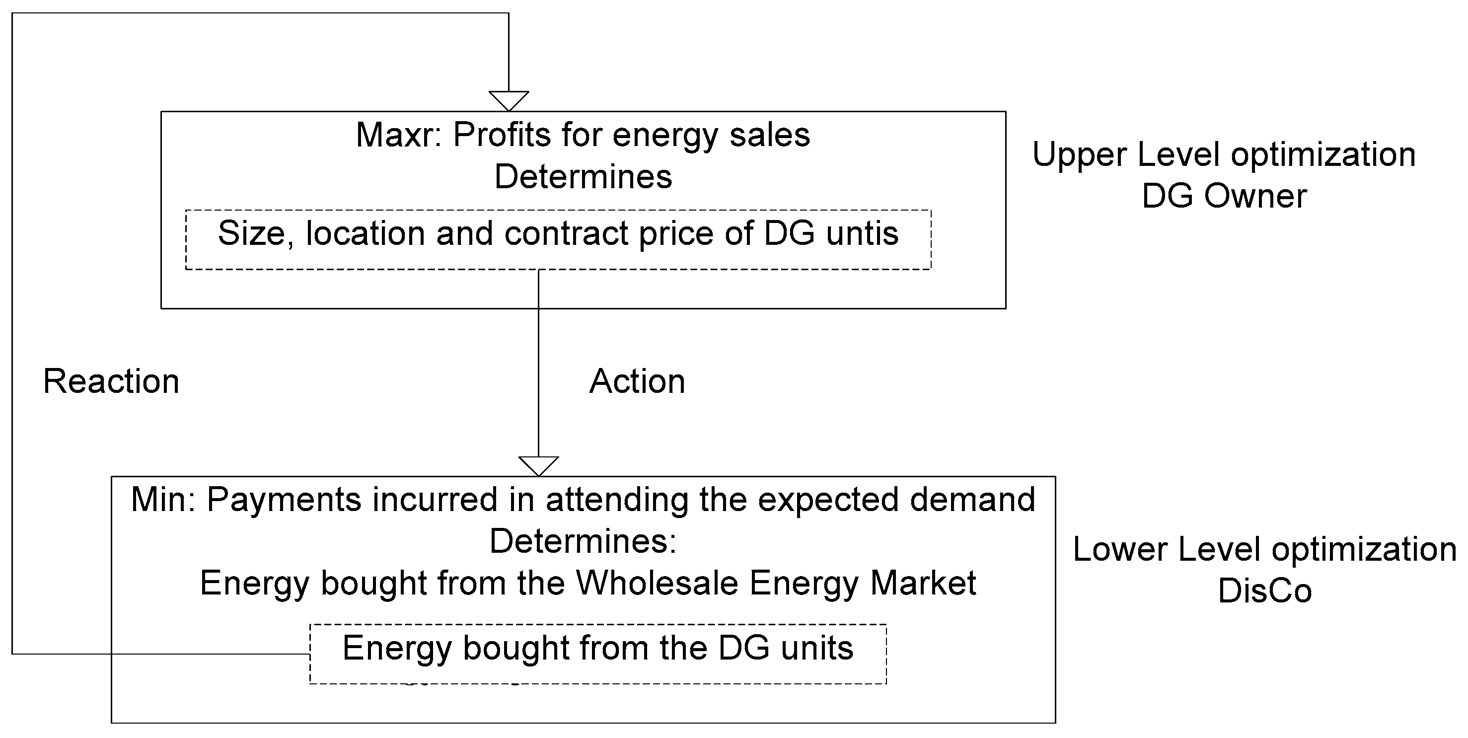
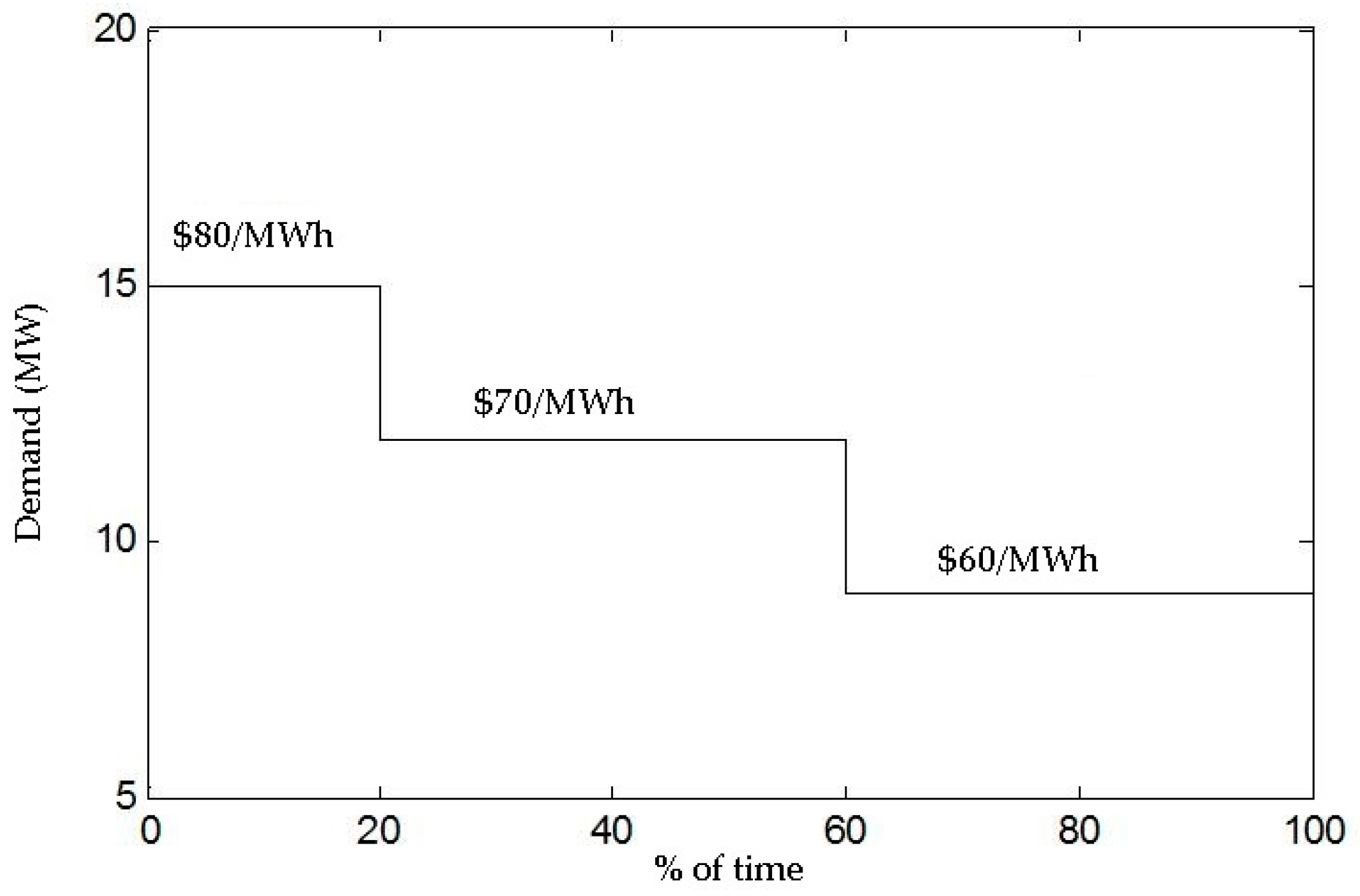
2.1. Decision-Making Problem of the Distribution Company

To meet the expected demand, the DisCo must decide on how much energy to purchase from the wholesale energy market and how much from the DG units within its network. At first glance, the easiest solution would be to buy energy from the cheapest source. However, the energy price is not the only factor that the DisCo must take into account when purchasing energy, since a power injection in an unsuitable bus might lead to problems such as overvoltage or an increase in power losses. Therefore, in order to account for network constraints, the DisCo must solve an optimal dispatch considering the presence of DG. For a given location and contract price, the solution of the optimal dispatch would yield the right amount of power to be purchased from the DG units and the wholesale energy market in order to minimize costs while meeting network constraints.

2.2. Decision-Making Problem of the Distributed Generation Owner

The objective function of the DG owner, considered in the proposed model, is the maximization of profits from the energy sales to the DisCo. In this case the DG owner must decide over the location, size, and contract price of the DG units. Also, he must take into account the reaction of the DisCo. Regarding contract price, negotiating a low energy price might result in more energy sales but not necessarily in more profits. As regards location, the owner of the DG must be aware of the fact that the impact of DG is highly dependent on the bus where it is located. Regardless of the energy price, the DisCo might not be willing to buy energy from the DG units if it has a negative impact on the network. Finally, the sizing of the DG is important, since it determines the investment costs and has a direct impact on the profits of the DG owner.

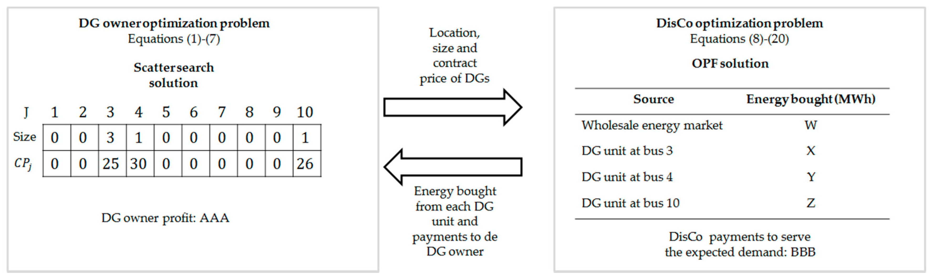
2.3. Bilevel Modeling Framework

The decision-making problems of both the DisCo and DG owner can be combined into a bilevel programming framework as shown in Figure 1. In this case, the upper level optimization problem corresponds to the DG owner; he must decide over the size, location, and contract price of the DG units (action). Once this information is known by the DisCo (located in the lower level optimization problem), he uses it as parameters for an optimal dispatch and determines the amount of energy he would be willing to purchase from the DG units (reaction). The DG owner now knows how much energy would be bought from his units, and is able to compute his expected profits. With this information, he might want to change his strategy testing new locations, contract prices, and sizes of DG. The process is repeated until an equilibrium is reached. That is, until there are not incentives for any of the agents to change their decisions. The idea behind this leader-follower game lies in the fact that the leader must consider the reaction of the follower before setting his strategy. That is, the DG owner takes into account the impact of the DG units in the network before deciding on their parameters. Equations (1)–(20) describe the mathematical model of the proposed methodology.

2.4. Upper Level Optimization Problem

The objective function of the upper level optimization problem consists on the maximization of profits of the DG investor given by (1). In this expression, $J$ represents the candidate locations for the DG units. The first term of the objective function corresponds to the income due to energy sales, where $C{P}_{DGj}$ is the contract price in $/MWh, associated to the $j^{th}$ DG unit; $P_{DGj}(t)$ is the power dispatched of the $j^{th}$ DG unit in time interval $t$ in MW; and $C_{DGj}$ is the production cost of the $j^{th}$ DG unit in $/MWh. Whereas the second term corresponds to the investment cost, where $I{C}_{DGj}(t)$ is the portion of the installation cost of the $j^{th}$ DG unit corresponding to time interval $t$; $P_{DGj}^{Max}$ is the size of the $j^{th}$ DG unit in MW and $\Delta t$ is the length of the time interval. The objective function given by (1) is subject to the minimum $(P^{Min})$ and maximum $(P^{Max})$ size limits of DG units, and the actual size selected ($P_{DGj}^{Max}$) (Equation (2)); and, the fact that the DG owner is willing to operate $k$ DG units (Equation (3)). Equations (4)–(6) define the decision variables for the location ($y_i$), size ($P_{DGj}^{Max}$) and contract price ($C{P}_{DGj}$) of each DG unit $j\in J$. Constraint (6) avoids selling energy from DG units that are not under operation. In this constraint, $C{P}^{max}$ represents the maximum admissible contract price. Finally, the reaction of the DisCo expressed in (7) represents the lower level optimization problem:

$$Max {{\displaystyle \sum }}_{t\in T}{{\displaystyle \sum }}_{j\in J}\Delta t\{ (C{P}_{DGj}-C_{DGj})P_{DGj}(t)-I{C}_{DGj}(t)P_{DGj}^{Max}\}$$

(1)

Subject to:

$$P^{Min}{y}_j\le P_{DGj}(t)\le P_{DGj}^{Max}\le P^{Max}{y}_j \forall j\in J; \forall t\in T$$

(2)

$${{\displaystyle \sum }}_{j\in J}{y}_i=k$$

(3)

$$y_i\in \{0,1\} \forall j\in J$$

(4)

$$P_{DGj}^{Max}\ge 0\forall j\in J$$

(5)

$$0\le C{P}_{DGj}\le C{P}^{max}{y}_i \forall j\in J$$

(6)

Reaction of the Distribution System Operator

(7)

2.5. Lower Level Optimization Problem

The lower level optimization problem (reaction of the DisCo) is given by Equations (8)–(20). For a given candidate solution of the DG investor regarding location, sizing, and contract pricing of the DG units, the DisCo reacts by purchasing a certain amount of energy from the DG units. The DisCo aims to minimize the cost of meeting the expected demand (8). The first term of Equation (8) corresponds to the cost of energy provided by the wholesale energy market; ${\rho }_{S{E}_k}(t)$ is the energy price at substation k in time interval t in $/MWh and $P_{SEk}(t)$ corresponds to the power provided to the network through substation k in time interval t. The second term of Equation (8) corresponds to the payments associated with the DG units within the DisCo’s network. Equations (9) and (10) correspond to active and reactive power balance constraints. $P_{G_n}(t)$ and $P_{D_n}(t)$ are the active power generated and demanded in bus n, in time interval t, respectively, while $P_n(t)$ corresponds to net active power injected in bus n in time interval t. $Q_{G_n}(t)$ and $Q_{D_n}(t)$ are the reactive power generated and demanded in bus n, in time interval t, respectively, while $Q_n(t)$ corresponds to net reactive power injected in bus n in time interval t. Equations (11) and (12) correspond to the expressions of active and reactive power injected in bus n, respectively. $G_{nm}$ and $B_{nm}$ are the real and imaginary entries in position (m, n) of the system admittance matrix; ${\theta }_{nm}(t)$ corresponds to the angle between buses n,m in time interval t and $V_n(t)$ corresponds to the voltage magnitude in bus n in time interval t. Equations (13) and (14) represent active power limits supplied by substations and DG units, upper scripts Max and Min stand for maximum and minimum limits, respectively. Equations (15) and (16) represent limits on reactive power and voltage magnitudes, respectively. Equation (17) represents apparent power limits in every line lnm. Equation (18) stands for the active and reactive components of apparent power. Equations (19) and (20) represent the mathematical expressions of active and reactive power flow on lines, respectively:

$$\min {\displaystyle \sum }_{t\in T}{\displaystyle \sum }_{k\in K}{\Delta }_t{\rho }_{S{E}_k}(t)P_{SEk}(t)+{\displaystyle \sum }_{t\in T}{\displaystyle \sum }_{j\in J}{\Delta }_{t}C{P}_{DGj}(t)P_{DGj}(t)$$

(8)

$$P_{G_n}(t)- P_{D_n}(t)-P_n(t)=0 ; {\forall }_n \in N , {\forall }_t\in T$$

(9)

$$Q_{G_n}(t)- Q_{D_n}(t)-Q_n(t)=0 ; {\forall }_n \in N , {\forall }_t\in T$$

(10)

$$P_n(t)= V_n(t){\displaystyle \sum }_{m \in N}{V}_m(t)\left[G_{nm}\cos {\theta }_{nm}(t)+ B_{nm}sin{\theta }_{nm}(t)\right]{\forall }_{n,m} \in N , {\forall }_t\in T$$

(11)

$$Q_n(t)= V_n(t){\displaystyle \sum }_{m \in N}{V}_m(t)\left[G_{nm}sin{\theta }_{nm}(t) - B_{n,m}cos{\theta }_{nm}(t)\right] {\forall }_{n,m} \in N , {\forall }_t\in T$$

(12)

$$P_{S{E}_k}^{Min}\le P_{S{E}_{k }}(t)\le P_{S{E}_k}^{Max} ; {\forall }_k \in K , {\forall }_t\in T$$

(13)

$$P_{DGj}^{Min}(t)\le P_{DGj}(t)\le P_{DGj}^{Max} ; {\forall }_j \in J , {\forall }_t\in T$$

(14)

$$Q_{S{E}_k}^{Min}\le Q_{S{E}_{k }}(t)\le Q_{S{E}_k}^{Max} ; {\forall }_k \in K , {\forall }_t\in T$$

(15)

$$V_n^{Min}\le V_n(t)\le V_n^{Max} ; {\forall }_n \in N , {\forall }_t\in T$$

(16)

$$-S_{lnm}^{Max}\le S_{lnm}(t)\le S_{lnm}^{Max} ; \forall l_{mn} \in L , {\forall }_t\in T$$

(17)

$$S_{lnm}(t)= P_{lnm}(t)+ j{Q}_{lnm}(t) ; \forall l_{mn} \in L , {\forall }_t\in T$$

(18)

$$P_{lnm}(t)= V_n^2(t)g_{nm}-V_n(t)V_m(t)g_{nm}\cos ({\theta }_{nm}(t))-V_n{V}_m{b}_{nm}sen({\theta }_{nm}(t)); \forall l_{mn} \in L , {\forall }_t\in T$$

(19)

$$Q_{lnm}(t)= - V_n^2(t)b_{nm}+V_n(t)V_m(t)b_{nm}\cos ({\theta }_{nm}(t))-V_n{V}_m{g}_{nm}sen({\theta }_{nm}(t)); \forall l_{mn} \in L , {\forall }_t\in T$$

(20)

For a given location, sizing and contract pricing of the DG units (upper level solution), the optimization problem given by (8)–(20) is basically an optimal dispatch.

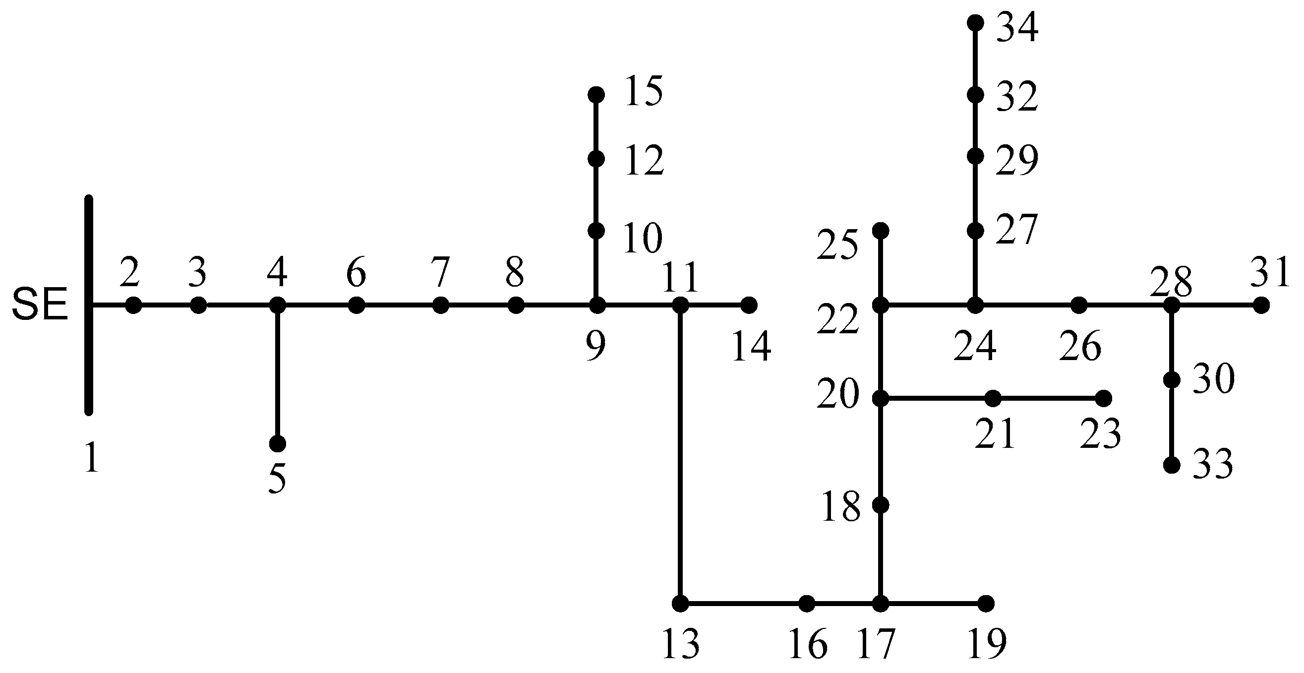
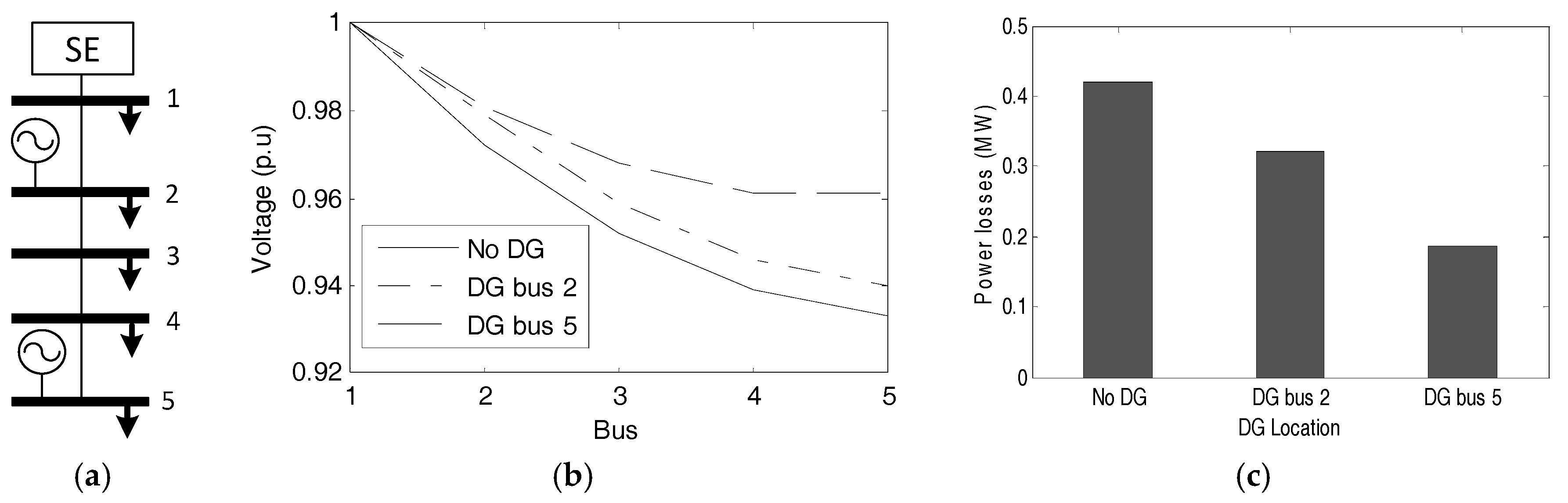
2.6. Illustrative Example

From an economic point of view, the straightforward solution for the DisCo would be to purchase energy from the cheapest source. However, the solution to the problem given by (1)–(20) is not that simple, since the DisCo must take into account not only the price of energy but also its impact in the network (power losses, voltage profile, congestion, etc.). An effective way to consider these aspects is by means of an optimal dispatch based on an AC optimal power flow. Figure 2 illustrates such a situation. Consider the 5-bus distribution system depicted in Figure 2a. A demand of 10 MW and 5 Mvar is considered for all buses, and an impedance of 0.01 + 0.1 j Ω is considered for all lines. Suppose that there is only one single DG unit to be allocated to either in bus 2 or bus 5 that provides the total demand of the bus. Both DG locations are advantageous to the DisCo in terms of improvement of voltage profile (see Figure 2b) and the reduction of power losses (see Figure 2c). However, it is evident that the DisCo would prefer the DG to be located in bus 5. If the DisCo is willing to pay a higher price for the energy supplied in bus 5 than for the one supplied in bus 2, there is an incentive for the DG investor to raise the price of the contract and propose the location of the DG unit in bus 5.

Within the bilevel programming scheme given by (1)–(20), the decision of the upper level problem would be to install a DG unit in bus 5 at a given energy price. With this information the DisCo evaluates the impact of such a DG unit solving the lower level problem given by (8)–(20). Note that in this case the DisCo considers technical (network limits) and economic issues (price offers). The solution of the lower level optimization problem determines how much energy the DisCo would be willing to buy from the DG owner. With this information, the DG owner determines his profits. Regarding DG size, there is a limit from which the DG creates counter flows and causes technical problems in the network. Such a situation, as well as other technical limitations can be accounted for as additional constraints in the lower level optimization problem.

3. Solution Approach

While genetic algorithms rely mostly on random decisions in their selection, crossover, and mutation operators, SS is a population-based heuristic that relies on deterministic procedures [28]. In power systems, SS applications include the planning of transmission network expansion [29], electric power load forecasting [30], and bi-objective environmental/economic dispatch [31].

Developed in the 1970s, recent applications of SS show its effectiveness to solve nonlinear optimization problems [32], and in optimization problems where the evaluation of the objective function implies costly computations (e.g., black-box optimization [33] and simulation optimization [34]). This advantage makes SS a good candidate for the solution of the bilevel optimization problem in models (1)–(20) since every feasible solution of (1)–(7) requires the solution of an optimal dispatch to find the reaction of the DisCo (problems (8)–(20)).

3.1. Scatter Search General Structure

SS combines and improves systematically the elements stored in a small reference set (RefSet) of good solutions found during the search process. Algorithm 1 depicts the general structure of the proposed SS for DG optimization.

Algorithm 1. Scatter search for DG optimization
1	$P=\varnothing$
2	While $\left|P\right|\le n$ do
3	$S= DiverseGeneration()$
4	If $S\notin P$ then
5	$P{\displaystyle \cup }\{S\}$
6	End-if
7	End-While
8	Evaluate the solutions in $P$ and sort them by non-increasing profit (Equation (1))
9	Build $RefSet$ with the best $b/2$ solutions of $P$, $RefSet=\{S_1,\dots S_{b/2}\}$
10	Add to $RefSet$ the most diverse $b/2$ solutions in $P$ with respect to those already in $RefSet$
11	Sort $RefSet$ by non-increasing profit (Equation (1))
12	$new=true$
13	While (new) do
14	$new=false$
15	For all $S and S_{}^{\prime }\in RefSet$ do
16	If ($S and S_{}^{\prime }$ has not been combined before) then
17	$\overline{S}=Combine(S,S^{\prime })$
18	$\overline{S}=Improve(S)$
19	$new=Update(RefSet,\overline{S})$
20	End-if
21	End-For all
22	End-While
23	Return $S^{\ast }=argma{x}_{S\in RefSet}\{f(S)\}$

As Algorithm 1 shows, SS initially builds a set $P$ of diverse solution using the diversification generation method (Lines 1–7). Once the number of desired diverse solutions ($n$) is reached, SS builds the initial $RefSet$ (Lines 8–11) with the best $b/2$ solutions in $P$. Moreover, to favor diversity, the remaining $b/2$ solutions added to $RefSet$ are those in $P$ more distant to solutions already in $RefSet$. Then, the main loop (Lines 13–22) of SS iterates until no new solutions are inserted in $RefSet$. This main loop follows three steps for all pairs of solutions in $RefSet$ (that includes at least one new solution): (i) combines the two solutions to obtain a new solution $\overline{S}$ (Line 17); (ii) applies the solution improvement method to $\overline{S}$ (Line 18); and (iii) tries to update the $RefSet$ by inserting $\overline{S}$ on it (Line 19). SS finishes when no new solutions are inserted in the $RefSet$. SS returns the best solution of the DG optimization problem in $RefSet$ (the solution with the largest profit for the DG owner) (Line 23).

3.2. Scatter Search Components

As it can be seen in Algorithm 1, the proposed SS uses four methods, namely: (i) diversification generator method ($DiverseGeneration$); (ii) solution combination method ($Combine$); (iii) improvement method ($Improve$); and (iv) reference set update method ($Update$). This section describes the details of each one of these methods. Likewise, two other important components for the SS implementation are discussed: the solution representation and the distance metric needed to maintain the diversity of the solutions in $RefSet$.

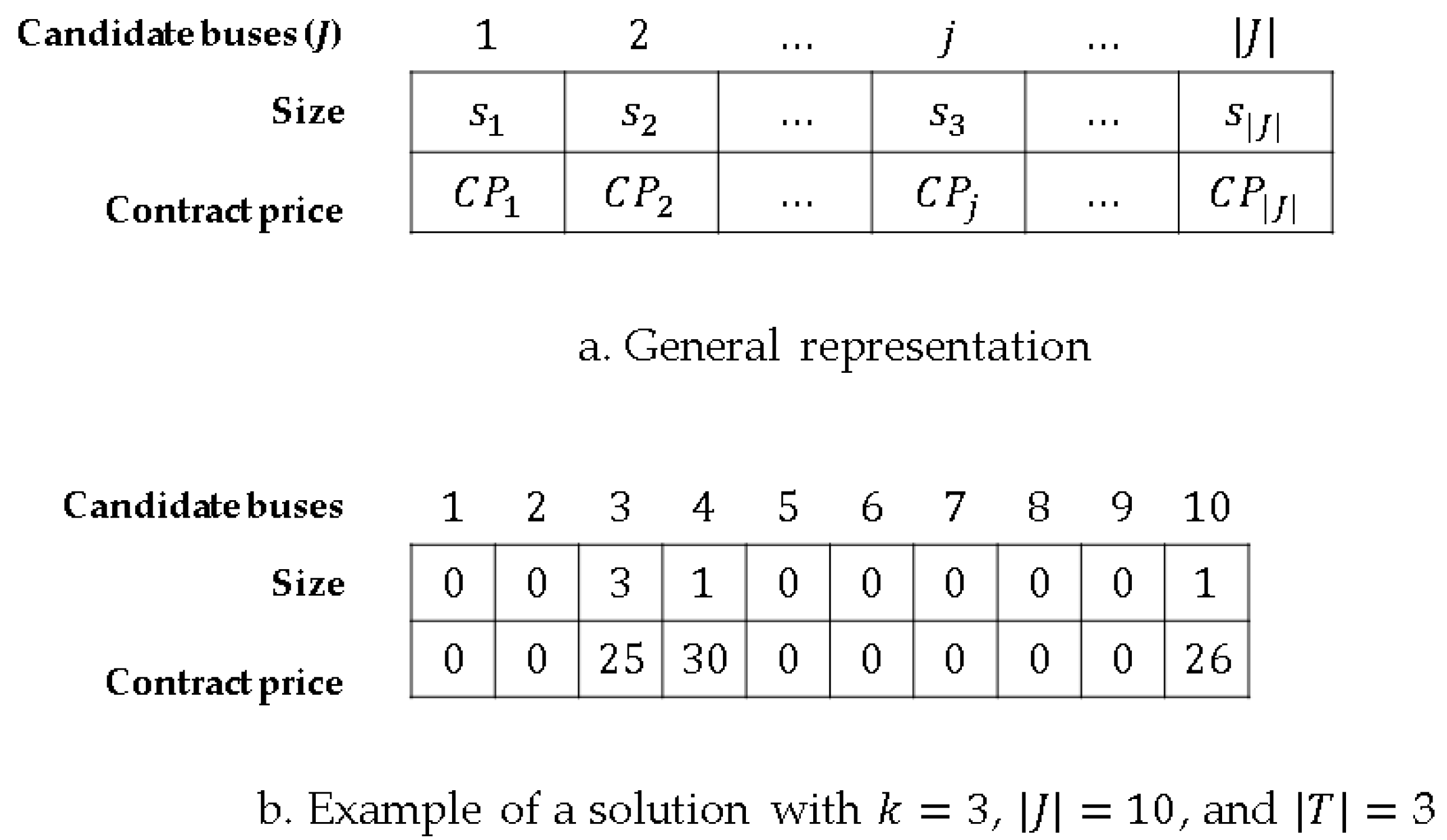
3.2.1. Solution Representation and Objective Function Evaluation

To represent the solutions of the DG optimization problem we use the two-row array depicted in Figure 3a. The position in the array correspond to the elements in $J$, the first row corresponds to the size of the DG located in the $j$-th element of $J$ ($P_{DGj}^{Max}$). To reduce the search space, the possible sizes of the DGs are constrained to a discrete set of options $T=\{P_{S1}=P^{Min},P_2, \dots ,P_{\left|T\right|}=P^{Max}\}$. Therefore, as can be seen in Figure 3, the first row indicates the index in $T$ and not the value of $P_{DGj}^{Max}$. On the other hand, the second row represents directly the contract price ($C{P}_{DGj}$) in monetary units. Figure 3b presents an example of a solution with 10 candidate buses in $J$ where the DG owner seeks to locate 3 DGs ($k=3$) with three possible sizes ($\left|T\right|=3$). In this solution DGs are located in the 3rd, 4th and 10th elements of $J$. The DG located at the 3rd candidate bus is of maximum size, whereas the two others are of the smallest possible size.

Figure 4 illustrates the evaluation process of the example solution of Figure 3. The leftmost part of Figure 4 presents the DG owner decisions for problems (1)–(7) (i.e., location, size, and contract price of their DG units). With this information, the DisCo (rightmost part of Figure 4) solves an optimal power dispatch (Equations (8)–(20)) to decide how much energy to buy from the wholesale market and the DG units to serve the expected demand at minimum cost. The DisCo returns this information to the DG owner so that he can calculate his profits (Equation (1)). This process repeats every time a new solution is found by the SS.

3.2.2. Distance Measure

SS seeks to balance the quality and the diversity of the initial set of solutions $P$ (Lines 9 and 10 of Algorithm 1). This creates the need to have a distance measure to compare the two solutions. To accomplish this task we use a simple distance measure that only compares the location of the DGs, ignoring the sizes and contract prices. The main motivation to ignore these two variables in the distance measure is the fact that the improvement operator modifies these variables. Therefore, after improvement, two solutions with the same locations for the DGs may result in the same local optima (with identical sizes and prices). For a given pair of solutions $S\mathrm{and}{S}^{\prime }$, the distance measure $dist(S,S^{\prime })$ operates in two steps. First, according to Equation (21), it uses the values of the first row of each solution to derive the binary variables ($y_j$), indicating whether or not a DG is located in candidate bus $j$. Then, in the second step it uses the Hamming distance of the location variables to calculate $dist(S,S^{\prime })$ using Equation (22). Where $y_j^S$ ($y_j^{S^{\prime }}$) indicates the value of the $y$ variable for the candidate bus $j$ is solution $S$ ($S^{\prime }$), respectively. Using $dist(S,S^{\prime })$ in Line 10 of Algorithm 1, we add sequentially the solution $S^d\in P$ that is more distant to all solutions already in $RefSet$ until completing $b$ solution (i.e., $S^d=argma{x}_{S^{\prime }\in P\backslash RefSet} \{mi{n}_{S\in RefSet} dist(S,S^{\prime })\}$):

$$y_j=\{\begin{array}{c}1 \mathrm{if} s_j\ge 0\\ 0 \mathrm{if} s_j=0\end{array}$$

(21)

$$dist(S,S^{\prime })={\displaystyle \sum }_{j=1}^{\left|J\right|}\left|y_j^S-y_j^{S^{\prime }}\right|$$

(22)

3.2.3. Diversification Generator Method

The first step of the SS generates a large set of diverse solutions $P$ of size $n$, from which it selects the initial solutions in $RefSet$ (Lines 2–7 of Algorithm 1). We consider three different diversification generator methods ($DiverseGeneration$). The first one is a completely random (Rand) method that selects randomly the location, size and price of the solutions in $P$. By contrast, the second one (Sist) generates diverse solutions in a deterministic way as follows. For the location, we use the procedure described in [35] that generates (systematically) binary vectors with $k$ values different from zero. Then, for the size we use the maximum size ($P_{\left|S\right|}$) and for the contract price also the maximum admissible price ($C{P}^{max})$. The third method (SistRand) combines the two previous ones by generating the location systematically according to [35], but generating the size and the contract price randomly.

3.2.4. Solution Combination Method

To combine pairs of solutions in $RefSet$ (Line 17 of Algorithm 1), we use only the location decisions (i.e., the $y$ variables). Therefore, we use again Equation (21) to derive the location decisions of a given solution $S$. Then, with the binary vectors of $y$ variables we apply a deterministic variant of the combination method for the knapsack problem described in [36] (p. 63). This combination method uses the objective function of the solutions $(f(S))$ to bias the selection towards the candidate locations of high-quality solutions.

Method ($Combine(S,S^{\prime })$) generates a new solution following four steps: (i) it calculates a score ($score(j)$) for each candidate location in $J$ according to Equation (23); (ii) then, it sorts the locations in non-decreasing order of the score; (iii) it picks the first $k$ to locate there the DGs; and finally; and (iv) it sets the size and contract price to random values as in the randomized diversification generation method:

$$score(j)=\frac{f(S)y_j^S+f(S^{\prime })y_j^{S^{\prime }}}{f(S)+f(S^{\prime })}$$

(23)

3.2.5. Improvement Method

Since the distance operator, diversification generation and combination methods focus on the location variables, we decided to apply the improvement method (Line 18 of Algorithm 1) to the other decisions of the DG optimization problem. Therefore, the improvement method ($Improve(\overline{S})$) applies a local search to the DG size ($P_{DGj}^{Max}$) or contract price ($C{P}_{DGj}$) of solution $\overline{S}$. Since the evaluation of a candidate solution implies the call of an (time-consuming) optimal dispatch, each time the improvement method is called, it operates with the same probability in only one of these decisions for a randomly selected DG of the solution. If the improvement is applied to the size (contract price), the method evaluates the increase/decrease of ±0.5 MW (±0.5 $/MWh) systematically until no more improvements can be achieved. For the initial solution, both increase and decrease of the size (contract price) are considered, and the direction (increase/decrease) with the larger improvement (if any) is selected for the next iterations. The local search stops as soon as no improvement is obtained or the minimum/maximum values for the variables are reached.

3.2.6. Reference Set Update Method

When trying to insert a new solution in the $RefSet$ (Line 19 of Algorithm 1), procedure $Update(RefSet,\overline{S})$ returns a Boolean value (new), that is true only if $\overline{S}$ is inserted in $RefSet$. The following condition must be valid to insert $\overline{S}$ in $RefSet: \exists S^{\prime } \in RefSet:f(\overline{S})>f(S^{\prime })$. That is, solution $\overline{S}$ must be better than at least one solution already contained in $RefSet$. As pointed out before, SS tries to balance the quality and the diversity of the solutions in $RefSet$. Therefore, once the update is successful (i.e., $new=true$) the distance measure is used to select which solution is replaced. In this case, the solution removed from $RefSet$ ($S^{out}$) is the closest to $\overline{S}$ with a worse objective function (i.e., $S^{out}=argmi{n}_{S^{\prime } \in RefSet:f(\overline{S})>f(S^{\prime })}\{dist(\overline{S},S^{\prime })\}$). The update of the reference set is then performed with the following operation: $RefSet$ = $RefSet{\displaystyle \cup }\{\overline{S}\}\backslash \{S^{out}\}$.

4. Tests and Results

The SS heuristic was implemented in Matlab. We used the Matpower software [37] to solve the optimal dispatch (Equations (8)–(20)) required to evaluate the reaction of the DisCo for each solution found during the search. After some preliminary experiments, we set the size of the initial population of diverse solutions ($P$) to $n=20$ and the size of the $RefSet$ to $b=6$. These small values provide short running times without compromising the solution quality. All of the experiments reported in this section were performed in a computer with an Intel Pentium processor with 2 GB of RAM running under Windows 7.

To evaluate the performance of SS we use a distribution system with 34 buses. Figure 5 depicts the structure of this system. Appendix A provides the detailed information of the buses, lines and demands of this system.

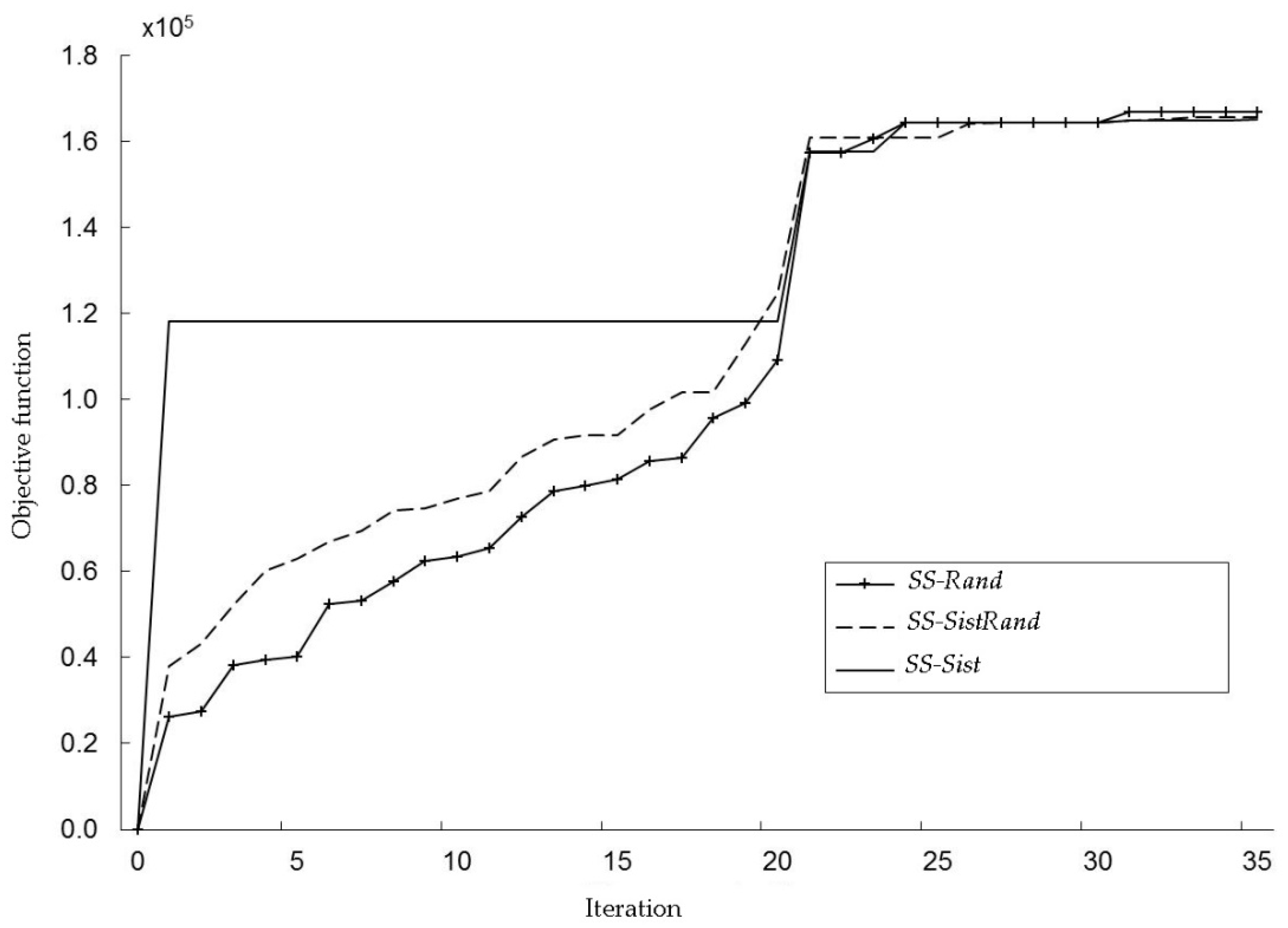
4.1. Diversification Generator Method Comparison

This first experiment compares the performance of the three diversification generation methods ($Sist, Rand and SistRand$), as described in Section 3.2.3. We performed three runs of each variant of the SS, with different seeds for the random number generator.

Table 1. Results for scatter search (SS) with different diversification generation methods.

SS Variant	DG Owner Profit			Average Running Time (s)	Best Profit
	Solution 1	Solution 2	Solution 3
SS-Sist	165,036	165,036	165,036	422	165,036
SS-Rand	165,952	166,303	166,731	407	166,731
SS-SistRand	165,339	165,484	165,119	607	165,484

and

Table 2. Best solutions of each SS variant for the 34-bus distribution system.

SS Variant	DG Unit (Bus, Price($/MWh), Size (MW))			DG Owner Profit
	1	2	3
SS-Sist	(24, 77.0, 1.5)	(29, 77.0, 1.5)	(30, 77.0, 1.5)	165,036
SS-Rand	(27, 77.0, 1.5)	(29, 77.0, 1.5)	(30, 77.0, 1.5)	166,731
SS-SistRand	(24, 77.0, 1.5)	(27, 77.0, 1.5)	(31, 77.0, 1.5)	165,484

present the results of this experiment. As it can be seen in Table 1, the randomized diversification generation method achieves the best results. Even its worst results outperform the other variants. As expected, the deterministic variant (SS-Sist) obtains the same results in all of the runs. The detailed information of Table 2 shows a convergence towards the same contract price and size in all of the best solutions, being the main difference the location of the DG units. This result can be explained by the effect of the improvement method, which searches for the best size and contract price, but does not affect the location of the DG units. Moreover, this result also supports the SS design that only takes into account the location of the DG units while combining and comparing the solutions in the RefSet.

Figure 6 depicts the results of the best runs of the three variants. As it can be seen, SS-Sist obtains very good results in the initial iterations, but is unable to improve the quality of the solutions in $RefSet$ during many iterations. On the other hand, the randomized variants begin with worst solutions but steadily improve their quality.

4.2. Comparison against Other Metaheuristics

In a second experiment, we compare the results of SS against those obtained with a memetic algorithm (i.e., a genetic algorithm hybridized with local search [38]). As a benchmark, we use the memetic algorithm (MA) developed in [39]. This MA extends the work of [21] to include the size of the DG as a decision variable. The general control of this MA is based on the work of Beasley and Chu [40]; as the SS, this MA uses a steady-state population replacement strategy, where only one chromosome is replaced in each iteration; furthermore, both heuristics share the solution representation and the improvement procedure (local search in the MA). On the other hand, there are several differences between the MA and the SS. First, while the MA uses a classical one-point crossover, the SS uses a deterministic voting procedure. Second, the MA relies on a (randomized) mutation operator to preserve the diversity of its population, whereas SS uses the distance measure and the reference set updating procedure as a mechanism to obtain a diverse $RefSet$. Third, while SS has a small reference set ($b=6$), the MA uses a large population with 100 chromosomes. Furthermore, to evaluate the impact of the solution improvement component (local search), we used as additional benchmark a simple genetic algorithm (GA). This simple method is obtained by removing the local search from the MA. Table 2 compares the results of the MA, the GA, and the proposed SS. For comparison we select the best and worst variants of the SS (SS-Rand and SS-Sist). Three runs of both methods were performed. Results for the MA and GA are taken from [39].

As it can be seen in

Table 3. Results for SS, memetic algorithm (MA) and genetic algorithm (GA) on the 34-bus distribution system.

Method	DG Owner Profit			Average Running Time (s)	Best Profit
	Solution 1	Solution 2	Solution 3
SS-Rand	165,952	166,303	166,731	407	166,731
SS-Sist	165,036	165,036	165,036	422	165,036
MA	156,128	157,601	155,423	302,400	157,601
GA	25,100	21,500	35,000	1200	35,000

, the proposed SS outperforms both the MA and the GA, both in solution quality and running time. The best SS solution offers 5.8% more profit to the DG owner than the best MA solution. Even the worst variant of SS (Sist) obtained solutions with 4.7% more profit. Remarkably, SS took a small fraction of the running time of the MA to reach better results (only 0.13% of the time of MA). According to [39], the MA took 3.5 h of running time on average to solve the DG optimization problem. Clearly, removing the local search from the MA produces a much faster method. The GA only took 20 min of running time on average. However, the quality of the solutions deteriorates. The best GA solution offers only 21% of the profit of the worst SS solution. Moreover, both methods were implemented in Matlab, but the MA experiments were run in a much faster computer with an Intel Core i5 processor (with 4 GB of RAM). These results show that SS offers a good option to solve DG optimization problems where the objective function evaluation consumes long running times.

5. Conclusions

This paper tackles the optimal location, sizing, and contract pricing of DG in electric distribution systems. To model this problem we follow a bilevel programming approach that considers the interaction between the DisCo and the DG owner.

These joint decisions (location, sizing, and contract price for the DGs) represent a challenge since the complexity of electric distribution systems hinders the application of exact optimization methods. Therefore, population metaheuristics like genetic algorithms and particle swarm optimization, among others, are one of the preferred options to solve this problem. As an alternative, this paper proposes a SS that relies (mostly) on deterministic mechanisms to preserve the quality and diversity of a small set of reference solutions.

Computational experiments on a test system with 34 buses reveal the effectiveness of the proposed SS. The comparison against a memetic algorithm and a genetic algorithm shows that the proposed heuristic is able to find better solutions in much shorter running times. The use of a small set of solutions and the deterministic diversity preserving mechanism of SS represent an advantage in problems where the objective function evaluation is a time-consuming task (as the DG optimization problem tackled in this paper).

Future research directions include the use of SS for multiobjective variants of the problem considering other performance measures (power losses, reliability, voltage stability, etc.), in addition to the DG owner profit. Likewise, the use of SS for the solution of other optimization problems that arise in the planning and operation of electric distribution systems (network configuration and reconfiguration, reliability optimization, etc.) appears as a promising alternative.

References

1. Liang, H.; Zhuang, W. Stochastic modeling and optimization in a microgrid: A survey. Energies 2014, 7, 2027–2050. [Google Scholar] [CrossRef]
2. Cheng, S.; Hu, W.; Zhang, X.; Chen, Z. Optimal reactive power and voltage control in distribution networks with distributed generators by fuzzy adaptive hybrid particle swarm optimization method. IET Gen. Trans. Dist. 2015, 9, 1096–1103. [Google Scholar] [CrossRef]
3. Gözel, T.; Hocaoglu, M.H. An analytical method for the sizing and siting of distributed generators in radial systems. Electr. Power Syst. Res. 2009, 79, 912–918. [Google Scholar] [CrossRef]
4. Hung, D.; Mithulananthan, N.; Basal, R.C. Analytical expressions for DG allocation in primary distribution networks. IEEE Trans. Energy Convers. 2010, 25, 814–820. [Google Scholar] [CrossRef]
5. Kang, H.K.; Chung, I.Y.; Moon, S.I. Voltage control method using distributed generators based on a multi-agent system. Energies 2015, 8, 14009–14025. [Google Scholar] [CrossRef]
6. Marwali, M.N.; Jung, J.W.; Keyhani, A. Stability analysis of load sharing control for distributed generation systems. IEEE Trans. Energy Convers. 2007, 22, 737–745. [Google Scholar] [CrossRef]
7. Piccolo, A.; Siano, P. Evaluating the impact of network investment deferral on distributed generation expansion. IEEE Trans. Power Syst. 2009, 24, 1559–1567. [Google Scholar] [CrossRef]
8. Cataliotti, A.; Cosentino, V.; Di Cara, D.; Russotto, P.; Telaretti, E.; Tine, G. An innovative measurement approach for load flow analysis in MW smart grids. IEEE Trans. Smart Grids. 2016, 7, 889–896. [Google Scholar] [CrossRef]
9. Bayindir, R.; Colak, I.; Fulli, G.; Demitras, K. Smart grid technologies and applications. Renew. Sustain. Energy Rev. 2016, 66, 499–516. [Google Scholar] [CrossRef]
10. Xavier, G.A.; Oliveira Filho, D.; Martins, J.H.; de Barros Monteiro, P.M.; Alves Cardozo Diniz, A.S. Simulation of distributed generation with photovoltaic microgrids—Case study in Brazil. Energies 2015, 8, 4003–4023. [Google Scholar] [CrossRef]
11. Jiang, Y.; Liu, C.; Xu, Y. Smart distribution systems. Energies 2016, 9, 297. [Google Scholar] [CrossRef]
12. Bai, H.; Miao, S.; Zhang, P.; Bai, Z. Reliability evaluation of a distribution network with microgrid based on a combined power generation system. Energies 2015, 8, 1216–1241. [Google Scholar] [CrossRef]
13. Colmenar-Santos, A.; Reino-Rio, C.; Borge-Diez, D.; Collado-Fernández, E. Distributed generation: A review of factors that can contribute most to achieve a scenario of DG units embedded in the new distribution networks. Renew. Sustain. Energy Rev. 2016, 59, 1130–1148. [Google Scholar] [CrossRef]
14. Colak, I.; Sagiroglu, S.; Fulli, G.; Yesilbudak, M.; Covring, C.F. A survey on the critical issues in smart grid technologies. Renew. Sustain. Energy Rev. 2016, 54, 396–405. [Google Scholar] [CrossRef]
15. Di Fazio, A.R.; Russo, M.; Valeri, S.; De Santis, M. Sensitivity-based model for low voltage distribution systems with distributed energy resources. Energies 2016, 9, 801. [Google Scholar] [CrossRef]
16. Armendariz, M.; Babazadeh, D.; Brodén, D.; Nordstrom, L. Strategies to improve the voltage quality in active low-voltage distribution networks using DSO’s assets. IET Gen. Trans. Dist. 2017, 11, 73–81. [Google Scholar] [CrossRef]
17. Zad, B.B.; Lobry, J.; Vallée, F. A centralized approach for voltage control of MV distribution systems using DGs power control and a direct sensitivity analysis method. In Proceedings of the IEEE International Energy Conference, Leuven, Belgium, 4–8 April 2016; pp. 1–6. [Google Scholar]
18. Kumar, A.; Gao, W. Optimal distributed generation location using integer non-linear programming in hybrid electricity markets. IET Gen. Trans. Dist. 2015, 9, 1096–1103. [Google Scholar] [CrossRef]
19. Rider, M.; López-Lezama, J.M.; Contreras, J.; Padilha, A. Bilevel approach for optimal location and contract pricing of distributed generation in radial distribution systems using mixed-integer linear programming. IET Gen. Trans. Dist. 2013, 7, 724–734. [Google Scholar] [CrossRef]
20. Soroudi, A.; Afraiab, M. Binary PSO-based dynamic multi-objective model for distributed generation planning under uncertainty. IET Renew. Power Gen. 2012, 4, 124–132. [Google Scholar] [CrossRef]
21. López-Lezama, J.M.; Contreras, J.M.; Padilha, A. Location and contract pricing of distributed generation using a genetic algorithm. Int. J. Elect. Power Energy Syst. 2012, 36, 117–126. [Google Scholar]
22. Abu-Mouti, F.S.; El-Hawary, M.E. Optimal distributed generation allocation and sizing in distribution systems via Artificial Bee Colony Algorithm. IEEE Trans. Power Deliv. 2011, 26, 2090–2101. [Google Scholar] [CrossRef]
23. Babu, M.A.; Mahalakshmi, R.; Kannan, S.; Karuppasamypandiyan, M.; Bhuvanesh, A. Application of self adaptive differential evolution algorithm for optimal placement and sizing of renewable DG sources in distribution network including different load models. Int. J. Adv. Eng. Technol. 2016, VII, 668–675. [Google Scholar]
24. Morad, M.H.; Abedini, M. A combination of genetic algorithm and particle swarm optimization for optimal DG location and sizing in distribution systems. Int. J. Elect. Power Energy Syst. 2012, 34, 66–74. [Google Scholar] [CrossRef]
25. Kefayat, M.; Ara, A.L.; Niaki, S.N. A hybrid of ant colony optimization and artificial bee colony algorithm for probabilistic optimal placement and sizing of distributed energy resources. Energy Convers. Manag. 2015, 92, 149–161. [Google Scholar] [CrossRef]
26. Prakash, P.; Khatod, D.K. Optimal sizing and siting techniques for distributed generation in distribution systems: A review. Renew. Sustain. Energy Rev. 2016, 57, 111–130. [Google Scholar] [CrossRef]
27. Abdmouleh, Z.; Gastli, A.; Ben-Brahim, L.; Haouari, M.; Al-Emadi, N.A. Review of optimization techniques applied for the integration of distributed generation from renewable energy sources. Renew. Energy 2017, 113, 266–280. [Google Scholar] [CrossRef]
28. Martí, R.; Laguna, M.; Glover, F. Principles of scatter search. Eur. J. Oper. Res. 2006, 169, 359–372. [Google Scholar] [CrossRef]
29. Mori, H.; Shimomugi, K. Transmission network expansion planning with scatter search. In Proceedings of the IEEE International Conference in Systems, Man and Cybernetics, Montreal, QC, Canada, 7–10 October 2007. [Google Scholar]
30. Mizutani, A.; Yukawa, T.; Numa, K.; Kuze, Y.; Iizaka, T.; Yamagishi, T.; Matsui, T.; Fukuyama, Y. Improvement of input-output correlations of electric power load forecasting by scatter search. In Proceedings of the 13th International Conference on Intelligent Systems Application to Power Systems, Arlington, VA, USA, 6–10 November 2005. [Google Scholar]
31. Costa e Silva, M.D.A.; Klein, C.E.; Mariani, V.C.; dos Santos Coelho, L. Multiobjective scatter search approach with new combination scheme applied to solve environmental/economic dispatch problem. Energy 2013, 53, 14–21. [Google Scholar] [CrossRef]
32. Ugray, Z.; Lasdon, L.; Plummer, J.; Glover, F.; Kelly, J.; Martí, R. Scatter search and local NLP solvers: A multistart framework for global optimization. INFORMS J. Comput. 2007, 19, 328–340. [Google Scholar] [CrossRef]
33. Gortázar, F.; Duarte, A.; Laguna, M.; Martí, R. Black box scatter search for general classes of binary optimization problems. Comput. Oper. Res. 2010, 37, 1977–1986. [Google Scholar] [CrossRef]
34. Laguna, M.; Marti, R. The OptQuest callable library. In Optimization Software Class Libraries; Voß, S., Woodruff, D.L., Eds.; Springer: New York, NY, USA, 2003; pp. 193–218. [Google Scholar]
35. Glover, F. A template for scatter search and path relinking. In Lecture Notes in Computer Science; Hao, J.K., Lutton, E., Ronald, E., Schoenauer, M., Snyers, D., Eds.; Springer: Berlin/Heidelberg, Germany, 1997; pp. 1–51. [Google Scholar]
36. Laguna, M.; Marti, R. Scatter Search: Methodology and Implementations in C; Springer: New York, NY, USA, 2003. [Google Scholar]
37. Zimmerman, R.D.; Murillo-Sanchez, C.E.; Thomas, R.J. MATPOWER: Steady-state operations, planning and analysis tools for power systems research and education. IEEE Trans. Power Syst. 2011, 26, 12–19. [Google Scholar] [CrossRef]
38. Krasnogor, N.; Smith, J. A tutorial for competent memetic algorithms: Model, taxonomy, and design issues. IEEE Trans. Evol. Comput. 2005, 9, 474–488. [Google Scholar] [CrossRef]
39. Buitrago, L.F. Ubicación, Dimensionamiento y Precio de Contrato Óptimo de Generación Distribuida en Sistemas de Distribución. Master’s Thesis, Universidad de Antioquia, Medellín, Colombia, 2014. (In Spanish). [Google Scholar]
40. Beasley, J.E.; Chu, P.C. A genetic algorithm for the set covering problem. Eur. J. Oper. Res. 1996, 94, 392–404. [Google Scholar] [CrossRef]
Figure 1. Bilevel programming framework.
Energies 10 01449 g001
Figure 2. (a) 5-bus distribution system; (b) impact of distributed generation (DG) location in voltage profile; and (c) impact of DG location in power losses.
Energies 10 01449 g002
Figure 3. Solution representation for scatter search (SS).
Energies 10 01449 g003
Figure 4. Objective function evaluation process.
Energies 10 01449 g004
Figure 5. 34-bus distribution system (Source [20]).
Energies 10 01449 g005
Figure 6. Progress of the best solution in RefSet for different scatter search variants.
Energies 10 01449 g006