
Forecasting of Chinese Primary Energy Consumption in 2021 with GRU Artificial Neural Network

1
Research Institute of Circular Economy, Tianjin University of Technology, Tianjin 300384, China
2
Department of Information and Library Science, Southern Connecticut State University, New Haven, CT 06514, USA
*
Author to whom correspondence should be addressed.
Energies 2017, 10(10), 1453; https://doi.org/10.3390/en10101453
Submission received: 17 July 2017
/
Revised: 28 August 2017
/
Accepted: 7 September 2017
/
Published: 21 September 2017
Abstract
:The forecasting of energy consumption in China is a key requirement for achieving national energy security and energy planning. In this study, multi-variable linear regression (MLR) and support vector regression (SVR) were utilized with a gated recurrent unit (GRU) artificial neural network of Chinese energy to establish a forecasting model. The derived model was validated through four economic variables; the gross domestic product (GDP), population, imports, and exports. The performance of various forecasting models was assessed via MAPE and RMSE, and three scenarios were configured based on different sources of variable data. In predicting Chinese energy consumption from 2015 to 2021, results from the established GRU model of the highest predictive accuracy showed that Chinese energy consumption would be likely to fluctuate from 2954.04 Mtoe to 5618.67 Mtoe in 2021.
1. Introduction
Energy is a vital resource needed for socio-economic development, and it is increasingly of concern to more and more governments and economic sectors because of its extensive application and the strong dependency on it in the processes of production and consumption [1]. In recent years, with the rapid development of the Chinese social economy and increase of population, there has been a rapid upward trend in Chinese energy demand and consumption [2]. Chinese main energy sources include hard coal, lignite, hydropower, oil, natural gas, geothermal, solar, wind, nuclear, etc., but efficiency of energy production and utilization is too low. In order to meet domestic energy demand, energy import trade volume is increasing year by year. Therefore, China should develop its own corresponding energy production plan to meet the rising domestic energy demand. To ensure energy security, it is important to predict annual energy consumption for a 5- to 10-year period to establish an appropriate energy plan. Energy consumption forecasting is affected by various aspects of socio-economic factors, among which the gross domestic product (GDP), population, import and export trade and other factors are particularly important [3].
The energy consumption model is usually based on historical consumption data and historical data related to energy consumption, such as the economy, population, climate, etc. [4]. At present, energy consumption forecasting in the world has three mainstream research methods: planning models, economic models, and machine learning models. The planning model uses linear and nonlinear programming to find the parameters that fit based on historical data. It was O’Neill who first applied the planning model to predict energy consumption in US [5]. Meanwhile, this method has also been applied in coal, oil, natural gas, power demand and other fields [6]. The economic model combines energy demand with other microeconomic variables and realizes the prediction of future energy demand through the inherent interaction between economic variables. The choice of economic variables is the key to the predicted accuracy [7]. The machine learning model breaks through the constraints of the original mathematical calculation in terms of the accuracy of prediction. It realizes and identifies the relationship between the data characteristics through artificial intelligence and realizes the prediction of future energy consumption through the modeling of a large amount of historical data. It identifies the relationships between the various data features by means of artificial intelligence. Therefore, the machine learning model realizes the prediction of future energy consumption based on the training of a large number of historical data. Moreover, there are many models of machine learning. The application of energy consumption includes Autoregressive Integrated Moving Average (ARIMA) model [8], Artificial Neural Network (ANN) model [9], Ant Colony Optimization (ACO) model [10], Particle Swarm Optimization (PSO) model [11] and so on.
In view of the dynamic change of energy consumption, Gated Recurrent Unit (GRU) can effectively solve the problem of error caused by the spatiotemporal evolution of energy consumption. It has gating units that modulate the flow of information inside the unit. Compared with the original machine learning method, GRU belongs to a deep learning method, as it can use the memory units in a network to deal with any data sequence of input. Therefore, the ability to learn time series of GRU is greatly superior [12]. The GRU may not only study the time series of long spans but also automatically determine the optimal time lag for prediction. In recent years, GRU has been successfully applied to handwriting recognition, human motion identification and robot control, etc. [13], but it is rarely applied in the field of economic forecasting. In this study, we selected three energy consumption forecasting models: multivariable linear regression (MLR), support vector regression (SVR) and Gated Recurrent Unit (GRU). By comparing these three models, we verified the superiority of the GRU model in the simulation of energy consumption from 2008 to 2015 in China. Then, we designed various scenarios to forecast Chinese primary energy consumption from 2015 to 2021. The results will help government to develop a reasonable energy plan.
2. Literature Review
2.1. Energy Consumption Forecast
In recent years, scholars from all over the world have studied the prediction of energy supply and consumption in the country and the region [14]. Sözen (2006) employed the artificial neural network method to obtain the formula to predict the net consumption of energy. The results showed that the error of the net consumption of energy consumption obtained via artificial neural network method was very small [15]. Deka (2016) compared five different forecasting technologies using economic and demographic factors to simulate US energy needs with in-depth discussion [16]. Torrini (2016) proposed a fuzzy logic approach to extract rules from input variables and to provide Brazil’s long-term annual electricity demand forecast [17]. Philip (2012) used ARDL and PAM to measure the short-term and long-term influencing factors of energy consumption in Ghana and forecasted Ghana’s energy consumption in 2020 [18]. Gokhan (2015) predicted Turkey’s primary energy consumption (PEC), which provided a predictive derivative model of population, gross domestic product (GDP) and energy consumption by regression analysis [19]. Some scholars combine energy consumption with carbon dioxide emissions to establish a correlation forecasting model. Hasiao (2012) applied the improved nonlinear gray model (Bernoulli) to analyze the characteristics of carbon dioxide emissions, energy consumption and actual output in China and to establish a predictive model of numerical iteration [20]. Pani (2010) applied correlation analysis to study the correlation of energy consumption, GDP and carbon emissions [21]. Wenying (2015) conducted a bottom-up analysis of energy consumption and carbon dioxide emissions from the Chinese steel industry [22]. Jain’s (2014) findings suggested that the sensor-based energy prediction model was suitable for multi-family residential buildings [23]. Wang (2011) analyzed the impacts of implementing new and expected energy and environmental policies with the Long-range Energy Alternatives Planning (LEAP) modeling tool [24]. Blanca Moreno (2016) used the combined model of grey neural network and input-output to predict primary energy consumption in the Spanish economic sector [25]. Xie (2015) applied the optimized single variable discrete grey prediction model to predict China’s total energy production and consumption, and proposed a new Markov method based on the quadratic programming model to predict the trend of China’s energy production and consumption structure [26].
2.2. Multiple Linear Regression
Multiple Linear Regression (MLR) is an important method in multivariate statistical analysis. It makes it possible to estimate the future regression coefficients and model accuracy without sampling the future system. At present, MLR is widely used in the research of many disciplines. Prakasvudhisarn (2015) predicted the electricity consumption of Thailand using the multiple linear regression and ANN models [27]. Abuella (2015) presented a multiple linear regression analysis model for solar power probabilistic forecasting [28]. Cleland (2010) applied multiple linear regression to usefully analyze the total energy consumption in the New Zealand food manufacturing industry [29]. Amral (2008) investigated the short-term load forecast of the demand of the South Suleai power system with the multiple linear regression method and concluded that the short-term load forecasting multiple linear regression model had been relatively easy to develop and regularly update, and was widely used in commercial computing software [30]. In Tuaimah’s (2014) research, the multiple linear regression method was used to present a short-term load forecast for Iraq’s power system requirements [31]. Torkzadeh (2014) applied multiple linear regression & principal component analysis (MLR-PCA) as the approach to predict weekly electrical peak load of Yazd city and concluded that the error of this proposed method was quite small [32]. Rahman (2014) presented a method for characterizing river water quality with the analysis of multiple linear regression [33]. Mata (2011) showed a comparison between the MLR and ANN models to characterize dam behavior under environmental loads [34]. Abushikhah (2011) proposed multivariable linear and non-linear regression, which used an hourly daily load to predict the next year’s hourly load, and the results obtained using the proposed method suggested that its performance was close [35].
2.3. Support Vector Machine
The Support Vector Machine (SVM) is an evolutionary algorithm for data exploration, and is an algorithm with a high prediction accuracy [36]. Support vector machines can be used to solve nonlinear programming problems, and can predict time series. At present, support vector machines have been widely used in planning, classification, nonlinear fitting and other fields. Its use is grounded in its superiority for solving nonlinear problems and, it has also applied to forecast energy consumption. Li (2009) applied SVM to predict the air conditioning energy consumption of office buildings. The results showed that the accuracy of SVM model prediction was higher than that of the BP neural network [37]. Hou (2009) predicted the air conditioning energy consumption of the (Heating, Ventilating, and Air-Conditioning) HVAC system, and the results showed that the SVM model was more accurate than the (Autoregressive Integrated Moving Average) ARIMA model [38]. Jain (2014) used the SVR model to predict energy consumption in New York’s multi-tenant buildings. Meanwhile, verifying temporal and spatial changes in particulate concentrations can have an impact on the accuracy of the forecast [23]. Wang (2015) tried to apply an instance-weighted variant of the SVM with both 1-norm and 2-norm formats to deal with the class imbalance problem [39]. Furthermore, Zhang (2013) studied the application of support vector machine in face recognition [40].
2.4. Gated Recurrent Unit
The Gated Recurrent Unit (GRU) changes the means of original supervising machine learning and solves the problem by carrying the memory unit of the forgotten mechanism. While the GRU deep learning model has drawn attention of late, its application is currently still relatively rare, and is mainly concentrated in computer-related areas. Le (2017) proposed a Gated Recurrent Unit (GRU) based on the Recurrent Neural Network (RNN) to construct an energy decomposition classifier with deep learning, and applied the method to training the model with the UK DALE dataset. From the experiment, Le concluded that the deep learning method was very effective for non-invasive load monitoring (NILM) [41]. Chung (2014) evaluated Recurrent Neural Networks (RNN) with three widely used recurrent units: a traditional tanh unit, a Long Short-Term Memory (LSTM) unit and a Gated Recurrent Unit (GRU). Finally, Chung confirmed the superiority of the Gated Recurrent Unit (GRU) [42]. Jozefowicz (2015) compared the GRU and LSTM models and found that the GRU model was able to achieve comparable results to the LSTM model on multiple issues, while the GRU model was easier to train [43]. Zhou’s experiments (2016) showed that GRU had some advantages in learning recurrent neural networks with stable performance and relatively few parameters [44]. Tang (2016) conducted an investigation on recurrent approaches to cope with question detection, and then built different RNN and bidirectional RNN (BRNN) models to extract efficient features based on gated recurrent units (GRU) at segment and utterance levels. Tang concluded that the particular advantage of GRU was that it can determine a proper time scale to extract high-level contextual features [45]. Rana’s (2016) speech experiments with eight different types of noise showed that the run time of the GRU was reduced by 18.16%, and was comparable to the long term short-term memory of the most popular recurrent neural network [46]. Huang (2017) verified the use of GRU-ELC units with the most advanced performance on three standard scene marker datasets. This comprehensive experiment showed that the new GRU-ELC unit facilitated the problem of on-site labeling because it could more effectively encode the longer context dependency in the image than the traditional RNN unit [47].
3. Research Methods
3.1. Multiple Linear Regression Model
The Multiple Linear Regression model is a method used to deal with the complex relationship between an output variable and multiple explanatory variables. The purpose of its analysis is to predict the output variables with the value of multiple explanatory variables. The main limitation of the model is that the correlation between the variables changes with time and space [48]. Assuming an output variable is , and some explanatory variables are , then the relationship between the output variable and the explanatory variable can be expressed as:
Meanwhile, is the value of the th explanatory variable for the year , is the constant term of the plan, is the parameter of the th explanatory variable, is the number of all explanatory variables, is the value of the output variable for year , is the estimated value of the output variable for year , is the prediction error, where can be defined as:
3.2. Support Vector Regression Model
The Support Vector Regression model obtains an approximate function from in the historical data sample of the correlated variable, which is already known. The data is mapped to a high dimension feature space by nonlinear method, and then the linear programming is carried out in this feature space [49].
In Equation (4), is the characteristic variable, and as coefficients that can be estimated from the data. In this way, the nonlinear programming of a low-dimensional input space can be deduced into a linear programming of high-dimensional feature space. The coefficient can be obtained with the minimum function:
In Equation (5), is a normalized constant, and function can be defined as:
The minimum function can also be expressed as follows:
Meanwhile, , , ; in addition, the kernel function explains the scalar product of the Di dimensional feature space:
The coefficients and can be obtained by the following formula:
The constraint is , , .
3.3. Gated Recurrent Unit Neural Network Model
The Gated Recurrent Unit (GRU) neural network model adapts to the problem of dependence on a variety of time scales by setting all kinds of cycle units [43] that modulate the flow of information with the gate unit. Assuming that the input of the model is expressed as , the logical calculation process is shown in Figure 1.
Assume that the activation function of GRU is a function related to time , which takes the linear interpolation between the activation function at the previous time point and the candidate activation function , which is :
At the same time, the update gate determines whether the unit updates the activation function or maintains the proportion and the number of the existing activation functions. The update gate is as follows:
The whole calculation process is to sum the existing state and the state of the update calculation, but the GRU model can’t control the range of state updates, but every calculation updates all of the states once.
The calculation of the candidate activation function is similar to that of the simple RNN calculation, and its computational function is:
Among which is the reset gate, is the vector product. When the reset door is closed (), the contents of the input sequence can be read while the past state is forgotten. The reset gate is calculated as follows:
The tanh function above has been very maturely and widely used in some research [45].
4. Data and Results Analysis
4.1. Data Sources
In order to verify the predictive accuracy of the above three models for Chinese primary energy consumption, in accordance with the research of Zong (2009) [50], we chose five variables: gross domestic product (GDP), population, import trade volume, export trade volume and energy consumption. Among these variables, the gross domestic product (GDP), population, import trade volume and export trade volume were regarded as independent variables, while energy consumption was a dependent variable. The data selected was from 1965 to 2015, and the data of the four variables of gross domestic product (GDP), population, import trade volume and export trade volume were derived from the World Development Indicator [51]. The Chinese primary energy consumption data was from the “BP World Energy Statistics Yearbook” [52]. These data are shown in Table 1. In this paper, the total number of data samples was 51. The 51-item data sample was used to divide the test samples from 15% of the total sample. The training samples were mainly used to modify the planning model, and the test samples were mainly used to judge the accuracy of the model. The experiment used 43 data items from 1965 to 2007 as training samples and 8 data items from 2008 to 2015 as test samples.
4.2. Analysis of Results
MLR and SVR models are deterministically mathematical methods, and stable results can be obtained according to the formulas given above. The GRU model is a deep learning neural network, and further constructs the model structure. The GRU model has three layers, including an input layer, a hidden layer, and an output layer. The input layer consists of four input variables: GDP, population, import, and export. The hidden layer consists of three GRU units with time steps of 1, 4, and 6, and each GRU unit contains 32 cells, and the output layer is the characteristic variable of primary energy consumption. The structure of the model is shown in Figure 2.
The training and testing of the GRU model were completed using the Keras kit on the PYTHON platform, in which the optimizer was set as “RMSprop”, the loss function was set as “MAPE”, the loss rate was set as “0.0001”, the epoch was set as 2000. In order to prevent the phenomenon of over-fitting, the calculation process was added to the validation part, determining whether or not it appears to be the best model parameters.
The main research goal of this paper is to compare the accuracy of the three models of MLR, SVR and GRU for medium term Chinese primary energy consumption forecasting. In order to express the advantages and disadvantages of the three models, the paper takes MAPE (mean absolute percentage error) and RMSE (root mean square error) as the results for error. The two error formulas are as follows:
At the same time, the in Equations (14) and (15) represents the actual primary energy consumption in China, while in the model represents the predicted value of Chinese primary energy consumption.
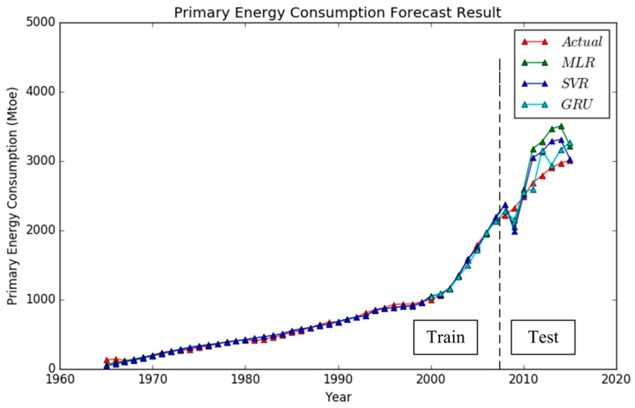
The experiments using MLR and SVR can be effectively performed, but when performing the experiment using GRU, a very interesting problem emerges. When using all the training data (1965–2007) to do the GRU prediction experiments, the error of the predicted MAPE is 14, which blocks the purpose of improving the accuracy of prediction. However, the error of the predicted MAPE is 5.63 when doing the GRU prediction experiment with the data of the first 8 years (2000–2007), allowing the emergence of the optimal prediction model parameters. The main reason for this situation is that the data input variables are in a state of annual growth. Recent data provides more information for the forecast results, whereas the earlier data will have a detrimental effect on the forecast. The training and test errors in Table 2 show that the GRU model has a higher accuracy in the prediction with the MAPE and RMSE indicators than that of MLR and SVR model in the comparison of the forecasting errors in Chinese primary energy consumption. Figure 3 shows the comparison between the actual value of primary energy consumption in China from 1965 to 2015 and the predicted values of various models. In summary, the GRU model is the best method of research to predict Chinese primary energy consumption; this model will be used in the prediction of Chinese primary energy consumption in the medium term.
5. Chinese Primary Energy Consumption Forecasts Based on Different Scenarios
After comparing the model errors, the GRU model was used to predict Chinese primary energy consumption from 2016 to 2021. An attempt was made to reduce the uncertainty of the forecast by setting appropriate scenarios, and by using the different scenarios with suitable forecast data. For gross domestic product (GDP), the forecast data of Chinese GDP published by the International Monetary Fund (IMF) [53] was employed. According to the World Population Prospects (2015) [54], the Chinese population will reach 1.424 billion by 2030. Using Equation (16) to calculate the annual growth rate of the population, it can be inferred that the Chinese approximate growth rate of the population from 2016 to 2021 will be 0.25%. Since there is no authoritative estimate of import and export trade in the world, the initial growth rate, average growth rate and minimum growth rate can only be calculated based on historical data of growth. Taking into account the potential for the country’s ongoing transformation and upgrading of the industry, the lowest growth rate is set at the lowest non-negative growth rate from 1965 to 2015. Due to the uncertainty of the import and export trade volume, the forecast of Chinese primary energy consumption from 2016 to 2021 is best set as four possible scenarios, as is shown in Table 3. According to the calculated method of the above data, Chinese gross domestic product and population estimations from 2016 to 2021 are shown in Table 4. The estimated data on Chinese import and export trade levels at different growth rates is shown in Table 5.
In Equation (16), is the annual growth rate, is the value of the beginning year, is the value of the ending year, the number of years in the whole phase is .
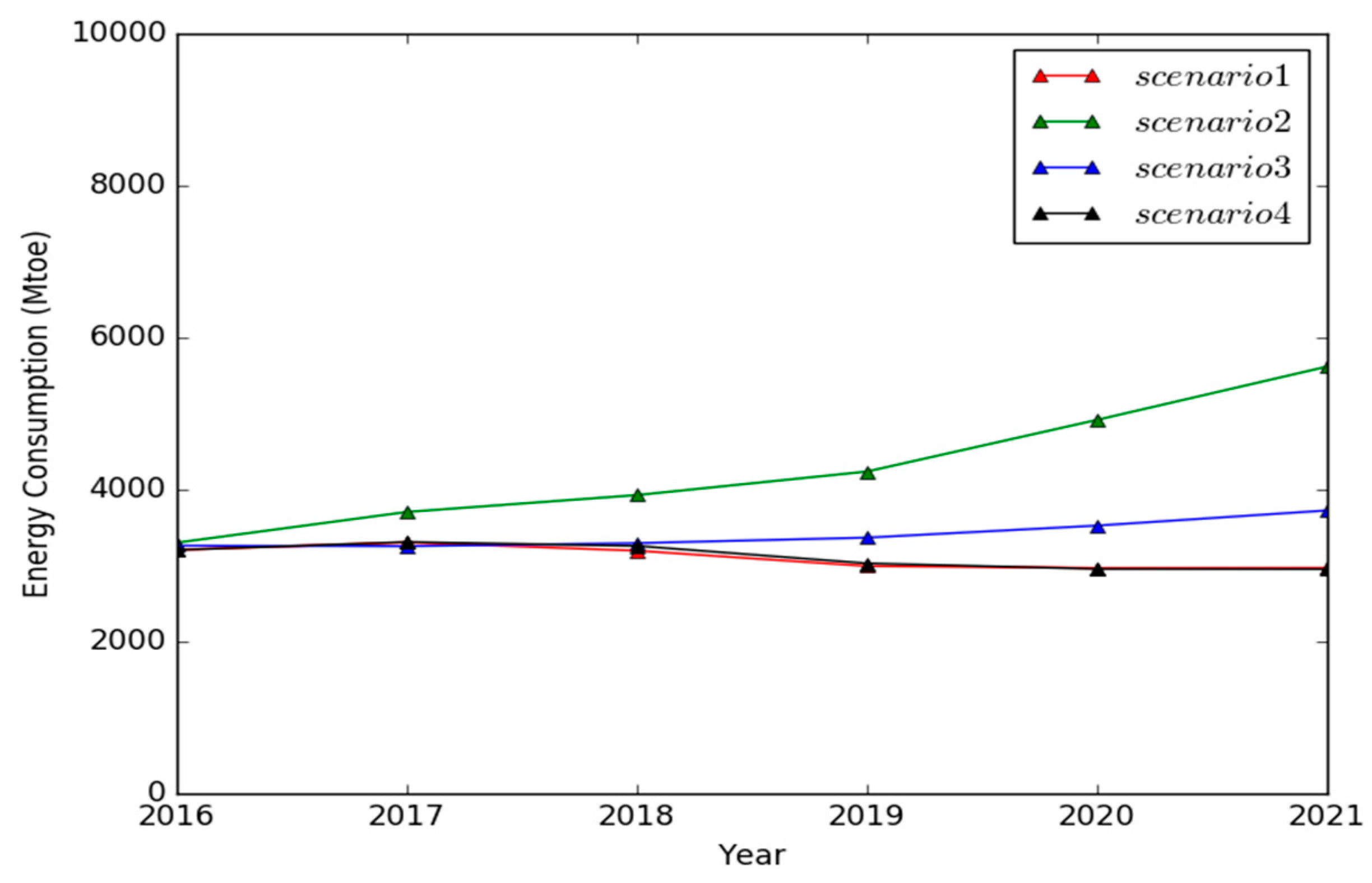
The data of four independent variables are substituted into the trained GRU energy consumption forecasting model; the results of the four different scenarios are compared in Figure 4.
Although more scenarios would more accurately assess the behavior of the predictive model in predicting possible Chinese energy consumption, the four scenarios were chosen from what realities have been appropriately assumed and computationally proven to achieve superior results, and hopefully represent the spectrum of possible consequences.
In Scenario 1, a negative growth of Chinese primary energy consumption is predicted from 3013.96 Mtoe in 2015 to 2970.19 Mtoe in 2021, cutting back 1.45% in 6 years. Calculated according to Equation (16), the annual growth rate is −0.24%.
In Scenario 2, Chinese primary energy consumption forecast indicates an increase of 86.42% from 3013.96 Mtoe in 2006 to 5618.67 Mtoe in 2021. According to Equation (16), the annual growth rate is 10.9%. Chinese primary energy consumption increases fastest in this scenario.
In Scenario 3, the forecast result of Chinese primary energy consumption suggests an increase of 23.6% from 3013.96 Mtoe in 2015 to 3725.2 Mtoe in 2021 and an annual growth rate of 3.6% based on Equation (16).
Scenario 4, China’s primary energy consumption forecast reveals a decrease of 3054.96 Mtoe from 2015 to 2954.04 Mtoe in 2021, with a decrease of 1.99% over six years. The annual growth rate is –0.33% according to Equation (16), and Chinese primary energy consumption witnesses the fastest decline in this scenario. To sum up, the four scenarios predict that Chinese energy consumption in 2021 will fluctuate between 2954.04 Mtoe and 5618.67 Mtoe.
The growing energy demand requires the government to make the right decisions in terms of energy planning. If energy planning results in incorrect underestimates of energy needs, there will be a shortage of energy supply, resulting in an energy deficit. Due to the strong correlation between energy consumption and greenhouse gas emissions, the prediction of future energy consumption can also affect the Chinese reaction to climate change. Through the accurate prediction of energy consumption, environmental managers can not only determine the major sources of carbon emissions, but can also determine whether all kinds of energy have an impact on climate change. Reliable energy forecasts can ensure the energy security of the country, achieving the sustainable development of energy and economy.
6. Conclusions
Chinese primary energy consumption forecasting is a key element of the success of national energy security and energy planning. Based on economic and demographic factors, three kinds of Chinese energy forecasting models—multivariable linear programming, support vector planning and gate recurrent unit—have been established for forecasting the energy consumption in China from 2016 to 2021. Through the results of the study, the following three important findings were obtained:
- Deep learning is the hotspot of current research, and in the GRU there are internal relations between the four economic variables (gross domestic product (GDP), population, import trade volume, export trade volume) and energy consumption. The four economic variables can be used to forecast the primary energy consumption in China;
- The GRU model is a model based on long and short memory for learning time series data. Compared with the MLR model and the SVR model, the GRU model is superior for the processing of time series data, and the average absolute percentage error of the predicted result can be as low as 5.63. However, when applying this model, the choice of the amount of training data is a key factor in accurate prediction. In particular, for the prediction of macroeconomic variables, recent data is more important to the final forecast result, due to uncertainties in socio-economic change; and
- The GRU model is used to forecast energy consumption in China from 2016 to 2021, with a finding that Chinese energy consumption in 2021 will fluctuate between 2954.04 Mtoe and 5618.67 Mtoe.
The proposed model could be one of the best techniques in deep learning. Although this is the first study that applies the GRU model in the prediction of Chinese primary energy consumption, there are more predictive testing technologies and methods that can be implemented. Two directions in the practice of the forecasting can be further pursued. First, continue to enhance the model structure and parameter settings of the GRU forecast method to increase the accuracy of the final energy consumption forecast; and second, select other economic variables related to energy consumption for the energy consumption forecast.
Acknowledgments
The funding sources of this work include the National Natural Science Foundation of China [grant number 71503180]; Ministry of Education Humanities and Social Sciences Project [grant number 13YJC630237]; Tianjin Science and Technology Development Strategy Research Project [grant number 15ZLZLZF00530]; Tianjin University Humanities and Social Sciences Project [grant number 20142101], Teaching Reform Project of Tianjin University of Technology [grant number YB12-21]; and Ministry of Education philosophy and social science research major research project [grant number 15JZD021].
Author Contributions
Bingchun Liu conceived and designed the experiments; Chuanchuan Fu performed the experiments; both together wrote the paper. Arlene Bielefield edited the paper. Yan Quan Liu contributed analysis tools and oversaw the manuscript’s content and production.
Conflicts of Interest
The authors declare no conflict of interest.
References
- Azadeh, A.; Saberi, M.; Ghaderi, S.F.; Gitiforouz, A.; Ebrahimipour, V. Improved estimation of electricity demand function by integration of fuzzy system and data mining approach. Energy Convers. Manag. 2008, 49, 2165–2177. [Google Scholar] [CrossRef]
- Delmastro, C.; Lavagno, E.; Mutani, G. Chinese residential energy demand: Scenarios to 2030 and policies implication. Energy Build. 2015, 89, 49–60. [Google Scholar] [CrossRef]
- Murat, K.; Adem, A.; Talat, S. Modeling and forecasting of Turkey’s energy consumption using socio-economic and demographic variables. Appl. Energy 2011, 88, 1927–1939. [Google Scholar]
- Egelioglu, F.; Mohamad, A.A.; Guwen, H. Economic variables and electricity consumption in Northern Cyprus. Energy 2001, 26, 355–362. [Google Scholar] [CrossRef]
- O’Neill, B.C.; Desai, M. Accuracy of past projections of US energy consumption. Energy Policy 2005, 33, 979–993. [Google Scholar] [CrossRef]
- Hao, Y.; Zhang, Z.Y.; Liao, H.; Wei, Y.M. China’s farewell to coal: A forecast of coal consumption through 2020. Energy Policy 2015, 86, 444–455. [Google Scholar] [CrossRef]
- Iniyan, S.; Suganthi, L.; Samuel, A.A. Energy models for commercial energy prediction and substitution of renewable energy sources. Energy Policy 2006, 34, 2640–2653. [Google Scholar] [CrossRef]
- Bakhat, M.; RossellÓ, J. Estimation of tourism-induced electricity consumption: The case study of Balearics Islands, Spain. Energy Econ. 2011, 33, 437–444. [Google Scholar] [CrossRef]
- Ekonomou, L. Greek long-term energy consumption prediction using artificial neural network. Energy 2010, 35, 512–517. [Google Scholar] [CrossRef]
- Toksari, M.D. Estimating the net electricity energy generation and demand using the ant colony optimization approach: Case of Turkey. Energy Policy 2009, 37, 1181–1187. [Google Scholar] [CrossRef]
- AlRashidi, M.R.; EL-Naggar, K.M. Long term electric load forecasting based on particle swarm optimization. Appl. Energy 2010, 87, 320–326. [Google Scholar] [CrossRef]
- Pezeshki, M. Sequence Modeling using Gated Recurrent Neural Networks. arXiv 2015. Available online: https://arxiv.org/abs/1501.00299 (accessed on 1 January 2015).
- Tang, D.; Qin, B.; Liu, T. Document Modeling with Gated Recurrent Neural Network for Sentiment Classification. In Proceedings of the 2015 Conference on Empirical Methods in Natural Language Processing, Lisbon, Portugal, 17–21 September 2015; pp. 1422–1432. [Google Scholar]
- Ahmad, A.S.; Hassan, M.Y.; Abdulan, M.P.; Rahman, H.A.; Hussin, F.; Abdullah, H.; Saidur, R. A review on applications of ANN and SVM for building electrical energy consumption forecasting. Renew. Sustain. Energy Rev. 2014, 33, 102–109. [Google Scholar] [CrossRef]
- Sözen, A.; Akçayol, M.A.; Arcaklioğlu, E. Forecasting Net Energy Consumption Using Artificial Neural Network. Energy Sources Part B Econ. Plan. Policy 2006, 1, 147–155. [Google Scholar] [CrossRef]
- Deka, A.; Hamta, N.; Esmaeilian, B.; Behdad, S. Predictive Modeling Techniques to Forecast Energy Demand in the United States: A Focus on Economic and Demographic Factors. In Proceedings of the ASME 2015 International Design Engineering Technical Conferences & Computers and Information in Engineering Conference, Boston, MA, USA, 2–5 August 2015. [Google Scholar]
- Torrini, F.C.; Souza, R.C.; Oliveira, F.L.C.; Pessanha, J.F.M. Long term electricity consumption forecast in Brazil: A fuzzy logic approach. Socio-Econ. Plan. Sci. 2016, 54, 18–27. [Google Scholar] [CrossRef]
- Philip, K.A.; William, B. Conditional dynamic forecast of electrical energy consumption requirement in Ghana by 2020: A comparison of ARDL and PAM. Energy 2012, 44, 367–380. [Google Scholar]
- Gokhan, A. Modeling of energy consumption based on economic and demographic factors: The case of Turkey with projections. Renew. Sustain. Energy Rev. 2015, 35, 382–389. [Google Scholar]
- Pao, H.T.; Fu, H.C.; Tseng, C.L. Forecasting of CO2 emissions, energy consumption and economic growth in China using an improved grey model. Energy 2012, 40, 400–409. [Google Scholar] [CrossRef]
- Pani, R.; Mukhopadhyay, U. Identifying the major players behind increasing global carbon dioxide emissions: A decomposition analysis. Environmentalist 2010, 30, 183–205. [Google Scholar] [CrossRef]
- Chen, W.; Yin, X.; Ma, D. A bottom-up analysis of China’s iron and steel industrial energy consumption and CO2 emissions. Appl. Energy 2015, 136, 1174–1183. [Google Scholar] [CrossRef]
- Jain, R.K.; Smith, K.M.; Culligan, P.J.; Taylor, J.E. Forecasting energy consumption of multi-family residential buildings using support vector regression: Investigating the impact of temporal and spatial monitoring granularity on performance accuracy. Appl. Energy 2014, 123, 168–178. [Google Scholar] [CrossRef]
- Wang, Y.; Gu, A.; Zhang, A. Recent development of energy supply and demand in China, and energy sector prospects through 2030. Energy Policy 2011, 39, 6745–6759. [Google Scholar] [CrossRef]
- Liu, X.; Moreno, B.; García, A.S. A grey neural network and input-output combined forecasting model. Primary energy consumption forecasts in Spanish economic sectors. Energy 2016, 115, 1042–1054. [Google Scholar] [CrossRef]
- Xie, N.M.; Yuan, C.Q.; Yang, Y.J. Forecasting China’s energy demand and self-sufficiency rate by grey forecasting model and Markov model. Int. J. Electr. Power Energy Syst. 2015, 66, 1–8. [Google Scholar] [CrossRef]
- Prakasvudhisarn, C. Electricity consumption forecasting in Thailand using an artificial neural network and multiple linear regression. Energy Sources Part B Econ. Plan. Policy 2105, 10, 427–434. [Google Scholar]
- Abuella, M.; Chowdhury, B. Solar power probabilistic forecasting by using multiple linear regression analysis. In Proceedings of the SoutheastCon, Fort Lauderdale, FL, USA, 9–12 April 2015; pp. 1–5. [Google Scholar]
- Cleland, A.C.; Earle, M.D.; Boag, I.F. Application of multiple linear regression to analysis of data from factory energy surveys. Int. J. Food Sci. Technol. 2010, 16, 481–492. [Google Scholar] [CrossRef]
- Amral, N.; Ozveren, C.S.; King, D. Short term load forecasting using Multiple Linear Regression. In Proceedings of the 2007 42nd International Universities Power Engineering Conference, Brighton, UK, 4–6 September 2007; pp. 1192–1198. [Google Scholar]
- Tuaimah, F.M.; Abass, H.M.A. Short-term electrical load forecasting for iraqi power system based on multiple linear regression method. Int. J. Comput. Appl. 2014, 100, 41–45. [Google Scholar]
- Torkzadeh, R.; Mirzaei, A.; Mirjalili, M.M.; Anaraki, A.S.; Sehhati, M.R.; Behdad, F. Medium term load forecasting in distribution systems based on multi linear regression & principal component analysis: A novel approach. In Proceedings of the 19th Electrical Power Distribution Networks (EPDC), Tehran, Iran, 6–7 May 2014; pp. 66–70. [Google Scholar]
- Rahman, A.U. Assessment of seasonal and polluting effects on the quality of river indus water by using multiple linear regression analysis. Int. J. Curr. Res. 2014, 6, 5005–5008. [Google Scholar]
- Mata, J. Interpretation of concrete dam behaviour with artificial neural network and multiple linear regression models. Eng. Struct. 2011, 33, 903–910. [Google Scholar] [CrossRef]
- Abushikhah, N.; Elkarmi, F.; Aloquili, O.M. Medium-term electric load forecasting using multivariable linear and non-linear regression. Smart Grid Renew. Energy 2011, 2, 126–135. [Google Scholar] [CrossRef]
- Wu, X.; Kumar, V. The Top Ten Algorithms in Data Mining; Taylor & Francis Group: New York, NK, USA, 2009. [Google Scholar]
- Li, Q.; Meng, Q.; Cai, J.; Youshino, H. Applying support vector machine to predict hourly cooling load in the building. Appl. Energy 2009, 86, 2249–2256. [Google Scholar] [CrossRef]
- Hou, Z.; Lian, Z. An Application of Support Vector Machines in Cooling Load Prediction. In Proceedings of the International Workshop on Intelligent Systems and Applications, Wuhan, China, 23–24 May 2009; Volume 26, pp. 1–4. [Google Scholar]
- Wang, X.; Liu, X.; Matwin, S.; Japkowicz, N. Applying instance-weighted support vector machines to class imbalanced datasets. In Proceedings of the IEEE International Conference on Big Data, Washington, DC, USA, 27–30 October 2015; pp. 112–118. [Google Scholar]
- Zhang, B.; Qiao, H. Face recognition with support vector machine. In Proceedings of the IEEE International Conference on Robotics, Intelligent Systems and Signal Processing, Changsha, China, 8–13 October 2003; pp. 726–730. [Google Scholar]
- Le, T.T.H.; Kim, J.; Kim, H. Classification performance using gated recurrent unit recurrent neural network on energy disaggregation. In Proceedings of the International Conference on Machine Learning and Cybernetics, Jeju, South Korea, 10–13 July 2016; pp. 105–110. [Google Scholar]
- Chung, J.; Gulcehre, C.; Cho, K.H.; Bengio, Y. Empirical evaluation of gated recurrent neural networks on sequence modeling. arXiv 2014. Available online: https://arxiv.org/abs/1412.3555 (accessed on 11 December 2014).
- Jozefowicz, R.; Zaremba, W.; Sutskever, I. An empirical exploration of recurrent network architectures. In Proceedings of the 32nd International Conference on Machine Learning (ICML-15), Lille, France, 6–11 July 2015; pp. 2342–2350. [Google Scholar]
- Zhou, G.B.; Wu, J.; Zhang, C.L.; Zhou, Z.H. Minimal gated unit for recurrent neural networks. Int. J. Autom. Comput. 2016, 13, 226–234. [Google Scholar] [CrossRef]
- Tang, Y.; Huang, Y.; Wu, Z.; Meng, H.; Xu, M.; Cai, L. Question detection from acoustic features using recurrent neural network with gated recurrent unit. In Proceedings of the IEEE International Conference on Acoustics, Speech and Signal Processing, Shanghai, China, 20–25 March 2016; pp. 6125–6129. [Google Scholar]
- Rana, R. Gated recurrent unit (GRU) for emotion classification from noisy speech. arXiv 2016. Available online: https://arxiv.org/abs/1612.07778 (accessed on 13 December 2016).
- Huang, Q.; Wang, W.; Zhou, K.; You, S.; Neumann, U. Scene labeling using gated recurrent units with explicit long range conditioning. arXiv 2017. Available online: https://arxiv.org/abs/1611.07485 (accessed on 28 March 2017).
- Armstrong, J.S. Illusions in regression analysis. Soc. Sci. Electron. Publ. 2012, 28, 689–694. [Google Scholar] [CrossRef]
- Müller, K.R.; Smola, A.J.; Rätsch, G.; Schölkopf, B.; Kohlmorgen, J.; Vapnik, V. Predicting time series with support vector machines. Lect. Notes Comput. Sci. 1997, 20, 999–1004. [Google Scholar]
- Zong, W.G.; Roper, W.E. Energy demand estimation of South Korea using artificial neural network. Energy Policy 2009, 37, 4049–4054. [Google Scholar]
- World Development Indicators. Available online: http://data.worldbank.org/data-catalog/world-development-indicators (accessed on 6 September 2017).
- Statistical Review of World Energy. Available online: http://www.bp.com/en/global/corporate/energy-economics/statistical-review-of-world-energy.html (accessed on 6 September 2017).
- Available online: http://www.imf.org (accessed on 6 September 2017).
- Available online: https://esa.un.org/unpd/wpp/publications/ (accessed on 6 September 2017).
Figure 1.
The computing logical of the Gated Recurrent Unit (GRU).
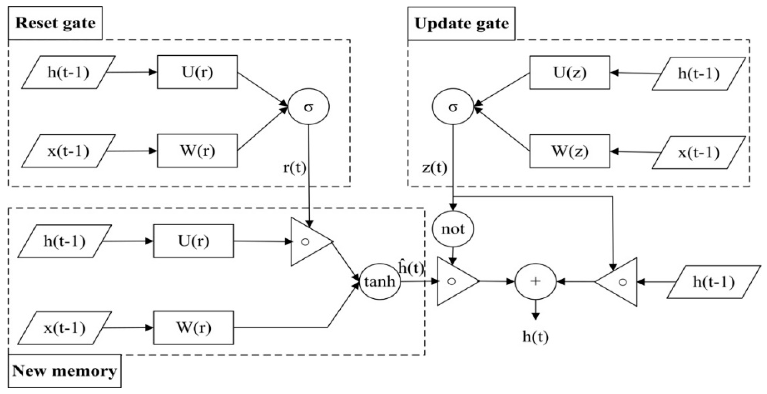
Figure 2.
The structure of GRU neural network.
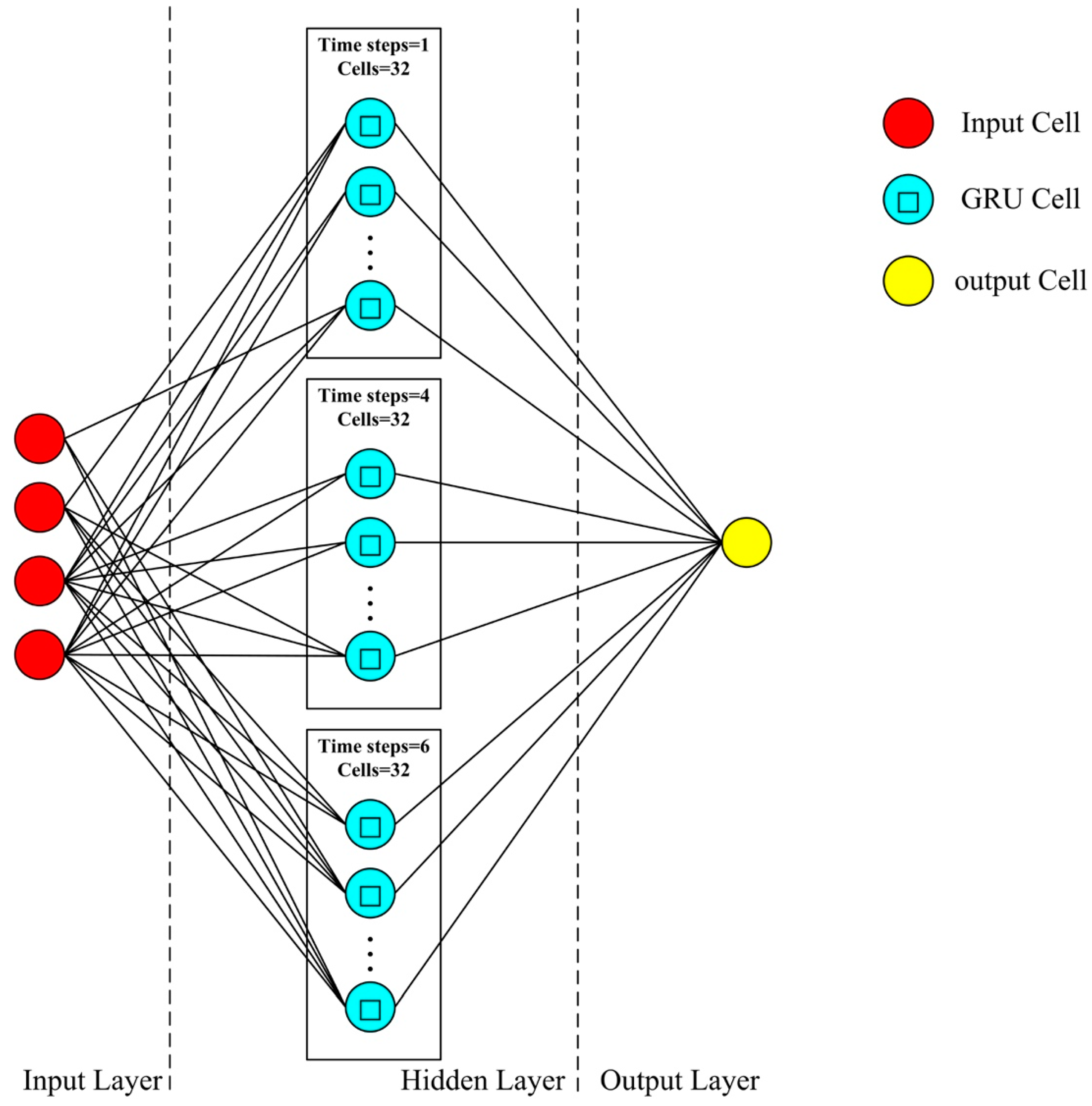
Figure 3.
Comparison of actual and predicted Chinese energy consumption (2008–2015).

Figure 4.
The forecasting results of Chinese energy consumption (2016–2021 year).

Table 1.
Primary energy demand and indicator data of China.
| Year | GDP (1010 Current US$) | Population (Million) | Import (109 Current US$) | Export (109 Current US$) | Primary Energy Demand (Mtoe) |
|---|---|---|---|---|---|
| 1965 | 6.97 | 715.19 | 2.25 | 2.56 | 131.40 |
| 1966 | 7.59 | 735.40 | 2.48 | 2.68 | 142.81 |
| 1967 | 7.21 | 754.55 | 2.17 | 2.39 | 128.44 |
| 1968 | 7.00 | 774.51 | 2.07 | 2.34 | 129.67 |
| 1969 | 7.87 | 796.03 | 1.92 | 2.43 | 157.87 |
| 1965 | 9.15 | 818.32 | 2.28 | 2.31 | 202.22 |
| 1971 | 9.86 | 841.11 | 2.13 | 2.78 | 239.79 |
| 1972 | 11.22 | 862.03 | 2.85 | 3.69 | 258.45 |
| 1973 | 13.68 | 881.94 | 5.21 | 5.88 | 272.69 |
| 1974 | 14.23 | 900.35 | 7.79 | 7.11 | 281.12 |
| 1975 | 16.12 | 916.40 | 7.93 | 7.69 | 314.91 |
| 1976 | 15.16 | 930.69 | 6.66 | 6.94 | 331.57 |
| 1977 | 17.23 | 943.46 | 7.15 | 7.52 | 361.68 |
| 1978 | 14.84 | 956.17 | 7.62 | 6.81 | 396.62 |
| 1979 | 17.69 | 969.01 | 10.56 | 9.20 | 408.16 |
| 1980 | 18.96 | 981.24 | 12.45 | 11.30 | 417.40 |
| 1981 | 19.44 | 993.89 | 14.59 | 14.59 | 411.58 |
| 1982 | 20.35 | 1008.63 | 13.65 | 15.79 | 429.53 |
| 1983 | 22.90 | 1023.31 | 16.16 | 16.79 | 456.86 |
| 1984 | 25.81 | 1036.83 | 22.16 | 20.73 | 490.18 |
| 1985 | 30.75 | 1051.04 | 42.78 | 27.51 | 529.92 |
| 1986 | 29.88 | 1066.79 | 43.43 | 31.37 | 555.31 |
| 1987 | 27.13 | 1084.04 | 36.19 | 32.96 | 598.77 |
| 1988 | 31.07 | 1101.63 | 42.29 | 36.35 | 643.12 |
| 1989 | 34.60 | 1118.65 | 44.53 | 39.60 | 674.60 |
| 1990 | 35.90 | 1135.19 | 49.22 | 57.09 | 681.41 |
| 1991 | 38.15 | 1150.78 | 59.21 | 66.67 | 716.17 |
| 1992 | 42.49 | 1164.97 | 69.75 | 73.41 | 753.24 |
| 1993 | 44.29 | 1178.44 | 74.63 | 65.88 | 810.25 |
| 1994 | 56.23 | 1191.84 | 115.56 | 120.92 | 858.79 |
| 1995 | 73.20 | 1204.86 | 132.30 | 149.11 | 884.98 |
| 1996 | 86.08 | 1217.55 | 139.01 | 151.26 | 932.17 |
| 1997 | 95.82 | 1230.08 | 142.42 | 182.88 | 936.95 |
| 1998 | 102.53 | 1241.94 | 140.43 | 183.88 | 938.18 |
| 1999 | 108.94 | 1252.74 | 165.93 | 195.21 | 969.67 |
| 2000 | 120.53 | 1262.65 | 225.15 | 249.26 | 1003.11 |
| 2001 | 133.22 | 1271.85 | 243.55 | 266.09 | 1059.63 |
| 2002 | 146.19 | 1280.40 | 295.16 | 325.58 | 1156.00 |
| 2003 | 164.99 | 1288.40 | 413.14 | 438.42 | 1347.98 |
| 2004 | 194.17 | 1296.08 | 561.04 | 593.26 | 1576.92 |
| 2005 | 226.86 | 1303.72 | 662.33 | 764.53 | 1793.70 |
| 2006 | 272.98 | 1311.02 | 794.86 | 973.21 | 1967.98 |
| 2007 | 352.31 | 1317.89 | 963.48 | 1230.72 | 2140.07 |
| 2008 | 455.84 | 1324.66 | 1144.48 | 1444.80 | 2222.28 |
| 2009 | 505.94 | 1331.26 | 1004.46 | 1200.77 | 2322.12 |
| 2010 | 603.97 | 1337.71 | 1380.08 | 1602.48 | 2487.36 |
| 2011 | 749.24 | 1344.13 | 1825.40 | 2006.30 | 2687.90 |
| 2012 | 846.16 | 1350.70 | 1943.22 | 2175.08 | 2795.26 |
| 2013 | 949.06 | 1357.38 | 2119.38 | 2354.25 | 2903.95 |
| 2014 | 1035.11 | 1364.27 | 2191.44 | 2475.70 | 2970.31 |
| 2015 | 1086.64 | 1371.22 | 2045.76 | 2431.26 | 3013.96 |
Table 2.
Comparison of forecasting error for various models.
| Model | MAPE | RMSE | ||
|---|---|---|---|---|
| Train | Test | Train | Test | |
| MLR | 5.55 | 12.8 | 26.39 | 392.84 |
| SVR | 5.91 | 9.17 | 27.95 | 284.08 |
| GRU | 2.11 | 5.63 | 5.45 | 12.4 |
Table 3.
The forecasting scenarios of Chinese energy consumption (2015–2021).
| Scenarios | GDP | Population | Import | Export |
|---|---|---|---|---|
| Scenario 1 | IMF’s forecast for Chinese GDP | The average population growth rate of China from the World Population Outlook (2015) (0.25%) | Initial growth rate (−6.65%) | Initial growth rate (−1.8%) |
| Scenario 2 | IMF’s forecast for Chinese GDP | The average population growth rate of China from the World Population Outlook (2015) (0.25%) | Average growth rate (16.49%) | Average growth rate (16.05%) |
| Scenario 3 | IMF’s forecast for Chinese GDP | The average population growth rate of China from the World Population Outlook (2015) (0.25%) | Minimum growth rate (1.52%) | Minimum growth rate (0.55%) |
| Scenario 4 | Chinese initial GDP growth rate (4.98%) | Initial population growth rate in China (0.5%) | Initial growth rate (−6.65%) | Initial growth rate (−1.8%) |
Note: The initial growth rate is the growth rate calculated in 2015, the average growth rate is the average growth rate from 1965 to 2015, and the minimum growth rate is the non-negative minimum growth rate from 1965 to 2015.
Table 4.
Chinese GDP and population estimation (2016–2021).
| Year | GDP (1010 Current US$) IMF Forecast Data | GDP (1010 Current US$) Initial Growth Rate 4.98% | Population (Million) Average Growth Rate 0.25% | Population (Million) Initial Growth Rate 0.5% |
|---|---|---|---|---|
| 2016 | 1158.36 | 1140.75 | 1374.65 | 1378.08 |
| 2017 | 1230.18 | 1197.56 | 1378.08 | 1384.97 |
| 2018 | 1303.99 | 1257.20 | 1381.53 | 1391.89 |
| 2019 | 1382.23 | 1319.81 | 1384.98 | 1398.85 |
| 2020 | 1463.78 | 1385.54 | 1388.45 | 1405.85 |
| 2021 | 1548.68 | 1454.54 | 1391.92 | 1412.87 |
Table 5.
China’s import and export estimation (2016–2021).
| Year | Import Trade Volume (109 Current US$) | Export Trade Volume (109 Current US$) | ||||
|---|---|---|---|---|---|---|
| Initial Growth Rate −6.55% | Average Growth Rate 16.49% | Minimum Growth Rate 1.52% | Initial Growth Rate −1.8% | Average Growth Rate 16.05% | Minimum Growth Rate 0.55% | |
| 2016 | 1911.76 | 2383.11 | 2076.86 | 2387.50 | 2821.48 | 2444.63 |
| 2017 | 1786.54 | 2776.08 | 2108.42 | 2344.52 | 3274.32 | 2458.08 |
| 2018 | 1669.52 | 3233.86 | 2140.47 | 2302.32 | 3799.85 | 2471.60 |
| 2019 | 1560.17 | 3767.12 | 2173.01 | 2260.88 | 4409.73 | 2485.19 |
| 2020 | 1457.98 | 4388.32 | 2206.04 | 2220.18 | 5117.49 | 2498.86 |
| 2021 | 1362.48 | 5111.95 | 2239.57 | 2180.22 | 5938.85 | 2512.60 |
© 2017 by the authors. Licensee MDPI, Basel, Switzerland. This article is an open access article distributed under the terms and conditions of the Creative Commons Attribution (CC BY) license (http://creativecommons.org/licenses/by/4.0/).
Share and Cite
MDPI and ACS Style
Liu, B.; Fu, C.; Bielefield, A.; Liu, Y.Q. Forecasting of Chinese Primary Energy Consumption in 2021 with GRU Artificial Neural Network. Energies 2017, 10, 1453. https://doi.org/10.3390/en10101453
AMA Style
Liu B, Fu C, Bielefield A, Liu YQ. Forecasting of Chinese Primary Energy Consumption in 2021 with GRU Artificial Neural Network. Energies. 2017; 10(10):1453. https://doi.org/10.3390/en10101453
Chicago/Turabian StyleLiu, Bingchun, Chuanchuan Fu, Arlene Bielefield, and Yan Quan Liu. 2017. "Forecasting of Chinese Primary Energy Consumption in 2021 with GRU Artificial Neural Network" Energies 10, no. 10: 1453. https://doi.org/10.3390/en10101453
Note that from the first issue of 2016, this journal uses article numbers instead of page numbers. See further details here.