Demand Response Unit Commitment Problem Solution for Maximizing Generating Companies’ Profit


Department of EEE, SRM University, Chennai 603203, India
*
Author to whom correspondence should be addressed.
Energies 2017, 10(10), 1465; https://doi.org/10.3390/en10101465
Submission received: 11 August 2017
/
Revised: 10 September 2017
/
Accepted: 19 September 2017
/
Published: 22 September 2017
(This article belongs to the Special Issue Distributed Energy Resources Management)
Abstract
:Over the recent years there has been an immense growth in load consumption due to which, Load Management (LM) has become more significant. Energy providers around the world apply different load management concepts and techniques to improve the load profile. In order to reduce the stress over the load management, Demand Response Unit Commitment (DRUC), a new concept, has been implemented in this paper. The main feature of this concept is that both the energy providers and consumers must participate in order to get mutual benefits hence maximizing each of their profits. In this paper we discuss the time-based Demand Response Program since there is no penalty observed in this program. When the Demand Response was combined with Unit Commitment and compiled it was observed that a satisfactory solution resulted, which is proved to be mutually beneficial for both Generating Companies (GENCOs) and their customers. Here, we have used a Cat Swarm Optimization (CSO) technique to find the solution for the DRUC problem. The results are obtained using CSO technique for UC problem with and without DR program. This is compared with the results obtained using other conventional methods. The test system considered for the study is IEEE39 bus system.

1. Introduction
With the improvements in the power sector field over the decades, there has also been a vast increase in load consumption due to heavy demand. Sometimes the load required is very high due to multiple consumers requiring power at the same time [1]. Due to this issue, GENCOs are sometimes not able to meet the customer demands, hence making them unsatisfied or prompting them to terminate their contracts. Some of the growing issues associated with power system operation include limited supply of system resources that in turn forces the operators to operate their systems at their maximum capacity, resulting in regular price hikes in the electricity market [2]. All the aforementioned limitations motivate us to search for and explore novel ways to increase the efficiency of resource utilization in power operations. As one of these new ways, Demand Response (DR) has recently become a major concept in power system operation. The use of Demand Response management in power systems enables the operators to efficiently utilize their resources as well as the power system operation. The use of Demand Response Programs (DRPs) in power system operation increases the profit of customers as well as the operators. It also encourages customers’ participation in the Demand Response Program (DRP) by rewarding them with incentives, if they agree to reduce their load demands during the peak hours of the day [3].
As per the Federal Energy Regulatory Commission (FERC), Demand Response can be defined as “Changes in electric usage by end-use customers from their normal consumption patterns in response to changes in the price of electricity over time, or to incentive payments designed to induce lower electricity use at times of high wholesale market prices or when system reliability is jeopardized” [4]. This is quite a different concept from energy efficiency that involves using less power for the same task. Demand response is also a component of smart energy demand that includes energy efficiency, home and building energy management, distributed renewable resources and electric vehicle charging [5]. The implementation of DRP in power system operation reduces the load stress on the equipment, hence ensuring a maximum efficiency and power. According to the Federal Energy Regulatory Commissions (FERC) report on demand response programs implemented in the US electricity markets from 2006 [6,7] DRP is broadly divided into two major categories:
(a) Time-Based Rate Programs (TBRP):
Time-Based Rate Programs (TBRPs) are programs that involve changes in the forecasted price that varies with the time of day, so the consumer can change or reduce their load usage for the respective hours accordingly. TBRPs are subcategorized into three programs, namely time of use, critical peak pricing and real time pricing programs. In time of use programs the main aim is to reduce the demand (peak periods) by increasing the prices at the high demand hour causing customers to shift or reduce their loads and lowering the prices where load management (off peak) use is possible. This attracts and encourages the customers to use load during off-peak hours. It is a basic type, where the rates of load per unit consumption vary in different time blocks. The rates during peaks are high and during off-peak periods are low [8]. Critical peak pricing rates consist of a pre-specified high load usage price imposed on Time of Use rates. These rates are applied for a short period of days or hours of a year. In real time pricing programs, the consumers are faced with hourly varying prices that reflect the real price of load in the market at that time. Customers under this program are informed in advanced about the prices on a day before or an hour before [9].
(b) Incentive-Based Programs (IBP):
IBPs are all based on paying or receiving a small amount in the form of penalties/incentives. IBPs are sub categorized into (i) Direct Load Control (ii) Emergency DR Program (iii) Demand Bidding/Buyback program (iv) Ancillary Services Program (v) Interruptible/Curtailable Service and (vi) Capacity Market program.
Direct Load Control involves programs where the loads are remotely controlled by the GENCOs, so they can be remotely committed or decommitted during peak hours in order to reduce the load stress. Some of the remotely controlled loads may include air conditioners, pumps and water heaters. Emergency DR Programs (EDR) require customers to curtail their loads during system emergencies [10]. The customers are in turn rewarded with incentives for curtailing their loads. In both Direct Load Control (DLC) and EDR programs, the customers are not penalized, if they fail to achieve the objectives, because they are involved in voluntary programs. In Demand Bidding/Buyback programs, the customers are encouraged to curtail load at a rate by which they are satisfied or how much load they are willing to curtail at the given price. In Ancillary Services Programs customers are made to bid and challenge their load curtailment values in markets as operating reserves [11].
Interruptible/Curtailable Service programs are the programs where the enrolled customers are asked to curtail their loads during the peak demand hours of a day in order to reduce load stress. They are in turn paid certain incentives to do so. If they fail to curtail the desired amount of load, they are penalized. In Capacity Market Programs, the customers are willing to perform pre-informed load curtailments for certain incentive rewards. Failing to do so will cause a penalization. Implementation of DR along UC not only reduces the load stress during peak hours, but it also increases the profits of GENCOs and makes the system more reliable. DR helps UC by shaving off loads during peak hours using various methods and thus causing an increase in profits and making systems more reliable and robust [12,13].
In order to implement demand response in smart grids, we should be able to coordinate large number of distributed resources using sensors, communication protocols and actuators. In addition, the increased presence of different renewable generation drives a much larger need for officials to procure more ancillary services in order to balance the grid [14,15]. Demand response is also provided by industrial customers. Industrial manufacturing plants’ magnitude of power consumption is very large compared to commercial and residential loads [16]. Demand response implementation was imposed in the United States by FERC Order No. 745 in March 2011 [4]. Reduction of loads during peak hours decreases the need for installing new units. According to the demand response smart grid coalition, around 10–20% of electricity costs are due to peak demand in the United States [17]. It was found in the California electricity crisis in 2000–2001 that lowering the demand by mere 5% would have resulted in a 50% of price reduction during peak hours [18]. A suit was filed regarding legality of order 745 by many affected parties, including the State of California [19]. From December 2009, the UK national grid has contracted to provide DR of 839 MW (35%) [20]. The mathematical formulation of the Market Clearing Model based on DRP was implemented in Singapore to improve the wholesale market profit [21]. The analysis on various power sectors of Germany was improved with wind power prediction [22].
The impact of UC and DRUC problems was studied by a dynamic approach on an IEEE 10 unit system [23]. Zhang et al. proposed how renewable energy resources can play a vital role in the future power system. How it can be used along with DR and electric vehicles in a UC problem to utilize wind power efficiently by using fuzzy chance constraints has also been studied [24]. The wind uncertainty can be overcome using ancillary services from Pumped Hydro Energy System (PHES) and DR and simultaneous scheduling of PHES and DR along with wind uncertainties has been attempted by solving an LR-based probabilistic UC [25].
The IBP based multi-objective energy management system is proposed in order to optimize micro grids by PSO [26]. Kwag et al. discussed virtual generation and the various costs reduction by using DR [27].The growing load factors in the Spanish electric energy system causing higher loads and increased cost and its reduction by demand shifting and curtailment were examined in [28]. The UC model is presented for accessing the reserve requirements resulting from large scale integration of renewable energy sources and deferrable demand in power systems and the alternative DR paradigms are discussed for accessing the benefits of demand flexibility in [29]. A robust optimization technique with wind power to derive an optimal UC was developed in [30]. Based on the explosion of fireworks in the sky, a unit commitment problem in a deregulated environment was modeled and the GENCOs’ profits were maximized [31]. An economic model of responsive loads is derived based upon price elasticity of demand and customers benefit function in [7]. Govardhan proposed a linear load economic model for solving the demand response unit commitment problem by using an Artificial Bee Colony algorithm [32]. The critical kick-back effect has been applied to a DR program for maximizing the profit in peak hours in a day in [33].
2. Demand Response Unit Commitment Problem Formulation
Traditional Unit Commitment (TUC) is the process of scheduling power generation, without violating the systems or units operational constraints. The traditional unit commitment problem objective function focuses on minimization of generation cost along with fuel costs and startup costs [32,34,35,36,37]. In this paper, the demand response based unit commitment problem is modeled and the main objective of the demand response unit commitment problem is used to maximize the profits of the GENCO using a Time-Based Demand Response Program (TBDRP) [38,39].
The objective function is as follows:
where, PR—is the total profit of the GENCOs and Demand Response Service Provider (DRSP) combined, TRV—is the total revenue calculated from the GENCOs and DRSP, TOCOST—is the total operating cost of the GENCOs and DRSP combined:
2.1. Mathematical Modelling of DRUC
The main objective of GENCOs in a deregulated environment is to maximize their profits, their objective being minimizing the cost of energy supplied to the consumers. Hence the traditional unit commitment is modeled with demand response program. The market clearing price in the demand response program is calculated from the DRSP supply curve coefficients and based on customer’s willingness to participate in a Demand Response Program. The demand response market clearing price is formulated by the following equation:
Here, μdi is the customer’s willingness to participate in a DR program. Its value is between 0 and 1, and the higher the willingness of customers, the less is the DR cost. θdi and δdi are DRSP coefficients for all customers [40]. Rewriting the above equation as:
where:
Rearranging the above equation, we get:
Equality must be maintained between the sold and purchased value of DR, and using this constraint the following equation is modeled:
The higher the willingness of customers to participate in DPR, the less will be the value of Δδdi. Similarly, the value of Δδdi increases as customer willingness decreases. The profit maximization equation for DRSPs is defined as:
Substituting and in Equation (11), we get:
where, the coefficients θmdi, δmdi and ϕmdi are referred to the customers’ supply curve cost coefficients. θdi is always considered equal to θmi. Taking derivation of the profit function with respect to Δδdi we get:
and:
Equating Equations (10) and (13) we get:
Rearranging the above equation, we get:
where:
2.2. Traditional Unit Commitment Constraints
2.2.1. Equality Constraint
2.2.2. Inequality Constraint
2.2.3. Ramp up Rate
2.2.4. Ramp down Rate
2.2.5. Minimum up Time
2.2.6. Minimum down Time
2.2.7. Reserve Constraints
2.2.8. Spinning Reserve
2.2.9. Startup Cost of Units
2.3. Demand Response Unit Commitment Constraints
2.3.1. Equality Constraint
2.3.2. Minimum up Time
2.3.3. Minimum down Time
2.3.4. Ramp up Rate
2.3.5. Ramp down Rate
3. Cat Swarm Optimization (CSO)
CSO optimization overcomes the limitations of PSO and DE that they are influenced by parameters and stagnation problem [41]. CSO is a meta-heuristic evolutionary optimization technique that intimates the natural behavior of felines. Cats have a strong curiosity towards objects that move. The cat group has superior hunting skills. Although it may be seen as always being at rest and they may seem to move slowly, they are always alert and aware of their surroundings [42]. Upon sensing the presence of prey, they chase it very quickly thereby spending a large amount of energy. These mentioned two characteristics, that is, the slow movement resting and sudden chase with high speed are described as seeking and tracking modes [43,44]. Each of these modes can be separately modeled mathematically.
3.1. Seeking Mode
There are four essential factors used in seeking, these factors are described as:
- (a)
- Seeking Memory Pool (SMP): number of copies of a cat produced.
- (b)
- Seeking Range of selected Dimension (SRD): difference between the new and old in the dimension selected for mutation.
- (c)
- Counts of Dimensions to Change (CDC): number of dimensions to be mutated.
- (d)
- Mixture Ratio (MR): to state that most of the time spent by the cats is resting and observing.
Steps executed in seeking mode:
- (1)
- Randomly select MR fraction of population as seeking cats: rest of them as tracing cats.
- (2)
- SMP copies of the ith seeking cat is created.
- (3)
- Update the position of each copy based on CDC by randomly adding or subtracting SRD fraction.
- (4)
- Evaluate error fitness values of copies.
- (5)
- Best candidate is picked from all copies and placed at ith seeking cat.
- (6)
- Repeat Step 2 until all seeking cats are involved.
3.2. Tracing Mode
This mode corresponds to the local search technique of an optimization problem. This method involves the cats tracing a target while spending a huge amount of energy. The rapid chase of cats is mathematically modeled as follows:
Define the position and velocity of ith cat in the D-dimensional space as:
and:
The global best position of a cat is represented as:
Updated equations are:
and:
The proposed method algorithm is given by the following steps:
- Step 1:
- Create N number of population.
- Step 2:
- Initialize time t = 0 and i = 0.
- Step 3:
- Find the overall cost and revenue for TUC and DRSP from the data provided using iterations and store the values and evaluate the profit for TUC and DRSP using the formula Pf = Rv − Tcost.
- Step 4:
- Check if all units are over and whether the cat is in seeking mode based on MR value
- Step 5:
- If yes, Seeking Mode.Create SMP copies and update position based on CDC, then take best value from SMP copies.
- Step 6:
- If no, then Tracing mode.Update position and velocity by using the equations:And save the highest profit unit.
- Step 7:
- Check if all cats are updated, if yes, then proceed or else go back to Step 4.
- Step 8:
- Check if maximum iteration is over, if yes, then stop and display the result, else go back to Step 2.
4. Result and Discussion
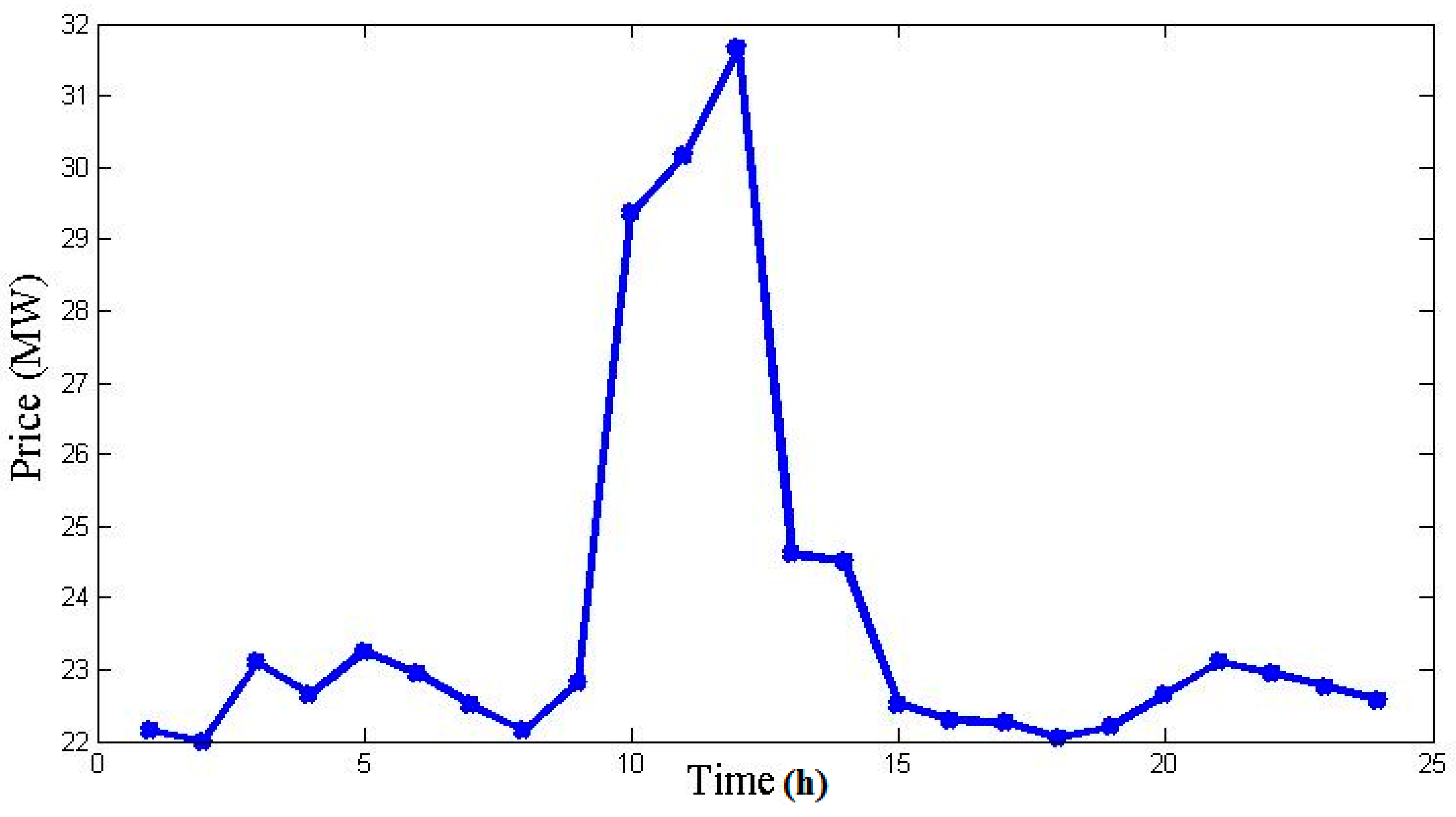
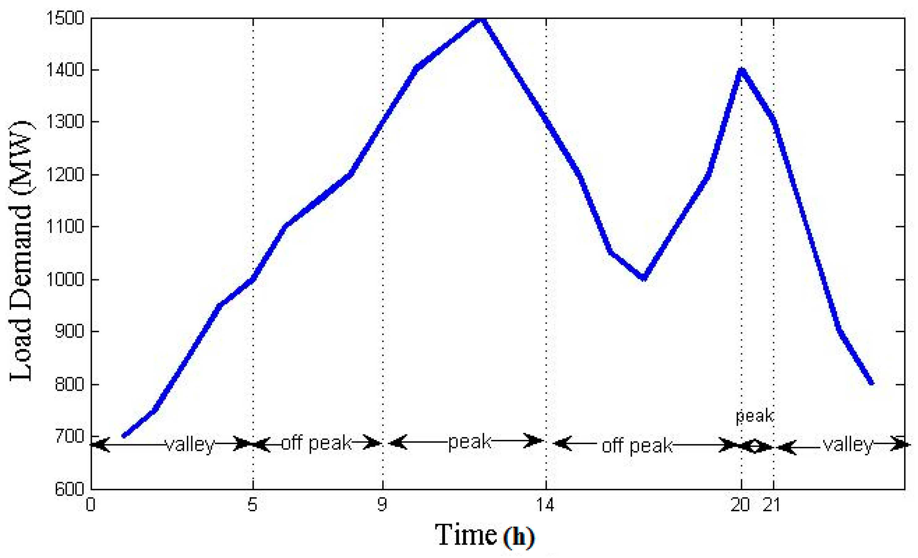
In this paper, we have used IEEE 39 bus system with conventional 10-units for a scheduling period of 24 h. The data for the load demand curve of the 10 unit systems is listed in Table 1. The operator data are listed in Table 2. The load data for the 10 unit 39 bus system is shown in Table 3. The forecasted price values for 24 h in a 10 bus system are shown in Table 4 and plotted in Figure 1. Six separate DRSPs are considered here, each generating load at a capacity of 50 MW. The load data curve value for these DRSPs is given in Table 5. The curve for forecasted price along with load demand variation for 24 h is plotted in Figure 2. Here it is noted that the price value during peak hours is high compared to the non-peak hours.
5. Simulation Results
The CSO formulation and solution methodology was implemented in MATLAB (2015, The MathWorks, Natick, MA, USA) and executed on a core i5 (2.6 GHz) personal computer equipped with 4 GB RAM. The proposed methodology that has been tested on a 10 unit generating system to solve TUC and DRUC problem is shown in Table 6, Table 7 and Table 8. The parameters assumed here are as follows; population size = 50, max iterations cycles = 100, SMP = 5, CDC = 0.6, SRD = 2, MR = 0.1, inertia weight w = 0.4 and acceleration constant C = 1.5 [41].
Two cases are considered for solving unit commitment problem.
5.1. Case 1: Base Case
In this case, TUC is formulated using CSO programming for the 10 unit generating system considering the initial loads. The output obtained for this is shown in Table 6. Here the total revenue generated is $651,380 and the total operating cost calculated is $563,937.7. The profit obtained with this TUC is $87,442.31, which is 13.42% as shown in Table 9. In Table 9 the average TUC profit of the proposed CSO method gives better results compared to the LR [45], BCGA, ICGA [46], BFA [47] and ICA [48] methods.
5.2. Case 2: Base Case Established Using DR
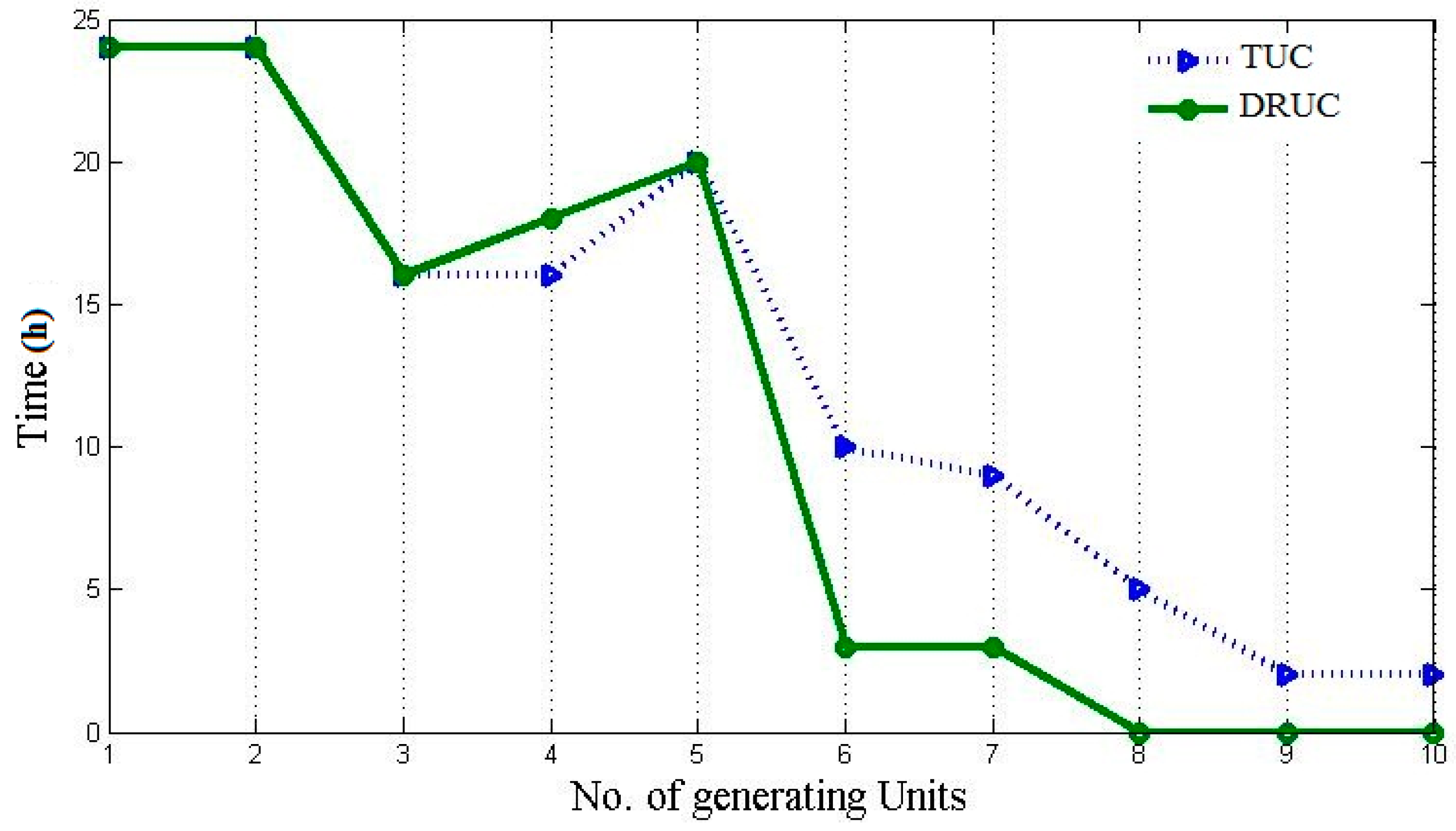
In this case, we have used a real time-based demand response program to reduce load during the peak hours of the day. The peak hours can be seen in Figure 2 where the various valleys, off peak and peak load hours are plotted. 20% of load is reduced only in those particular hours and a TUC problem is executed and the output is shown in Table 7. The total revenue generated is $593,389.50 and the total operating cost calculated is $507,954.30. The profit obtained here is $85,435.21 as shown in Table 9. In the output Table 7, it is seen that the generators 8, 9 and 10 are not committed thereby reducing the total operating cost. The various generator running hours are depicted in Figure 3. From Figure 3, it is observed that the TUC methodology uses the entire generators in its distribution hence causing rise in cost. Whereas in DRUC the last three units are idle and don’t take part in generation hence reducing the overall cost.
Along with this TUC programming, the six separate DRSPs that were installed are now used for generation. These generators generate the 20% load that was reduced from the initial case for their corresponding hours, respectively. The output of these generators are shown in Table 8. The same forecasted price given in table 4 is used to calculate the revenue. The revenue generated for these hours is $57,990.5, and the total operating cost is $40,512.5 for DRSP. The total revenue obtained when combined with the DRUC and DRSP is $651,380. This is same as that of our base case hence proving the same value of price is considered in our proposed case too as shown in Table 9. The total operating cost is $548,466.80. This is lower than our base case hence increasing the profit to $102,913.20 (15.8%), thus giving a profit rise of 2.37% shown in Table 9. Even an amount as low as a dollar saved per day will sum up to be much greater amount at the end of a year, although upon comparison, the amount doesn’t seem to be much higher, but considering long term generation, it will make a huge difference.
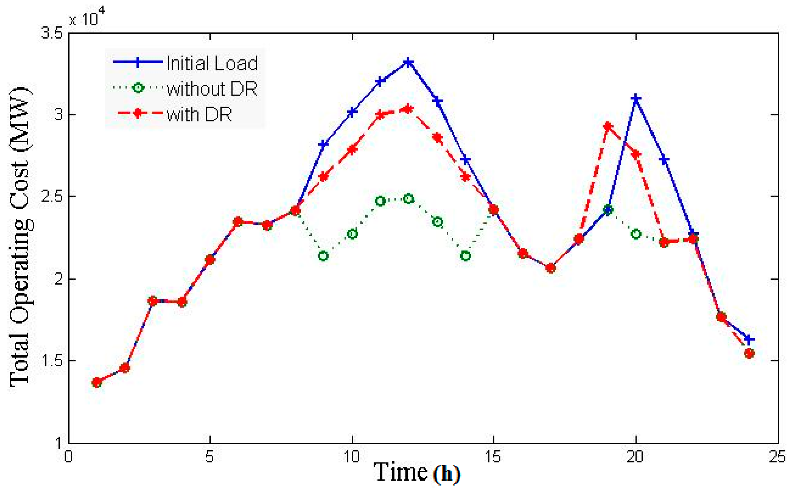
The cost comparison for the base case and the base case with DR and DRSPs is shown in Figure 4. The base case is observed to have the maximum cost while the base case with DR has less due to the reduced load during the peak hours. The final case being the total cost combined of base case with DR and DRSPs. It is noticed that the profit is maximum when DRUC is scheduled rather than TUC. The various running data for the separate DGs installed is shown in Figure 5. It is observed that all the units are committed for peak hours and generating 50 MW each, except for the last unit, that is varied throughout peak hours in order to equalize the demand power.
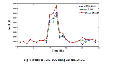
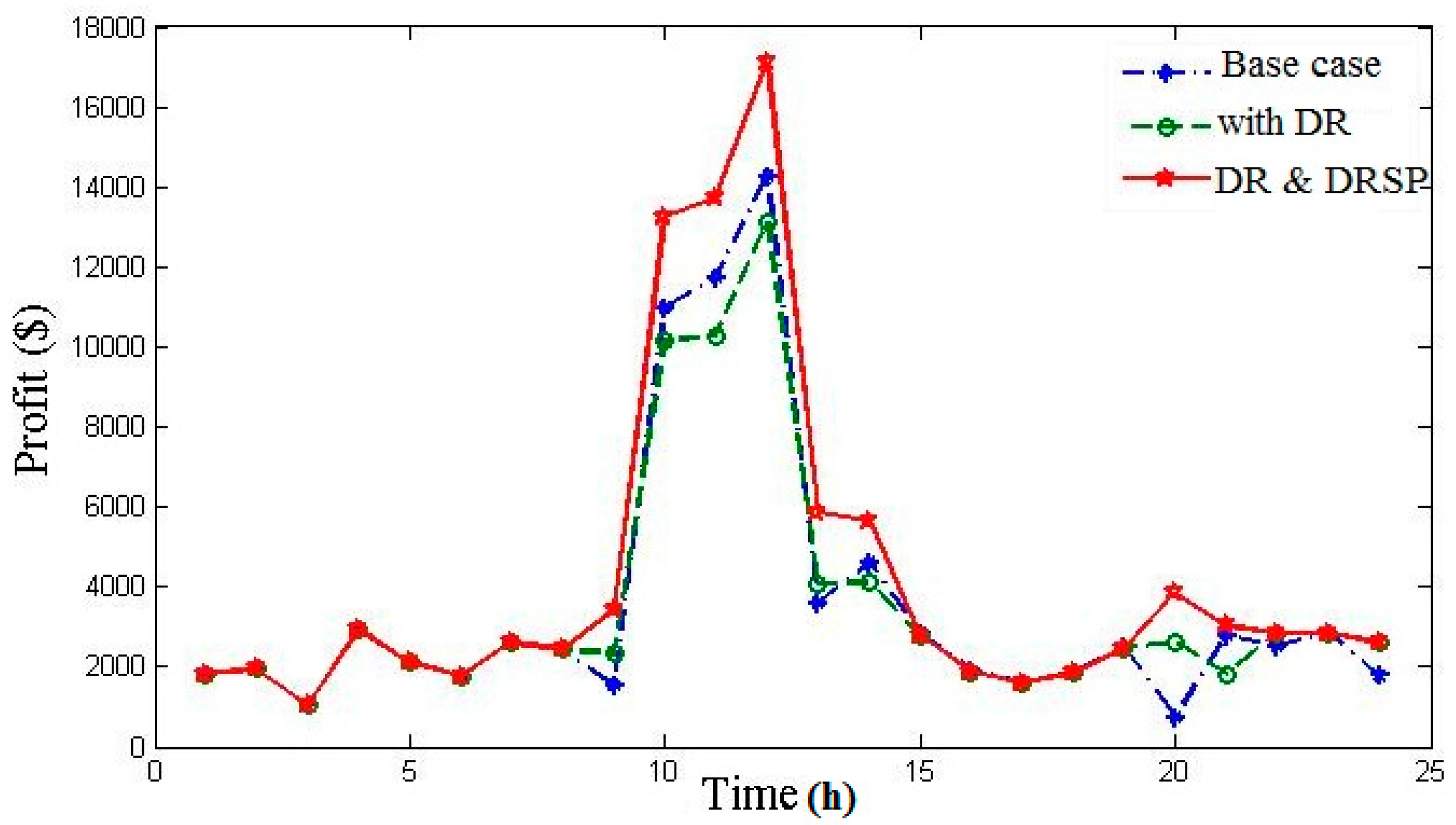
The load demand versus time curve is depicted in Figure 6. The peak time load has been reduced using DRUC when compared with TUC. The reduced load value is generated by the DRSP’s which is shown in Figure 5. The profit calculated for base case, base with DR and DRSPs are shown in Figure 7.
It is noted that the profit is more using DRUC when compared with TUC. Also the curve when only the base case with DR excluding DRSPs is plotted and depicted. The various revenues calculated in TUC and DRUC are shown in Figure 8.
It can be seen that the revenue when DR is established is reduced. This reduced revenue is calculated for DRSPs using the same spot price values. It should be noted that the revenue for both cases are one and the same. The total operating cost for the base case, base case using DR without DRSPs and base case using DR with DRSPs are shown in Figure 9. It is observed that the overall cost is reduced in DRUC when compared with TUC.
6. Conclusions
In this paper, a demand response-based unit commitment model is solved using the Cat Swarm Optimization technique. A real time-based demand response program is used here to reduce load stress during peak hours and reduce the overall cost of the generation system. Also, six Demand Response Service Providers are used to compensate for the reduced load values. It is observed that using demand response unit commitment maximizes the profit for both GENCOs and the Demand Response Service Providers. Even though the load is reduced during peak periods the GENCOs gain higher percentage of profit. The consumer gains profit by installing DRSPs that supply the shaved-off loads during peak hours thereby decreasing the overall cost and maximizing the profit. From the simulation studies, although the revenue remains the same in TUC as in DRUC, it is observed that by implementing DRUC in generation systems, there is an overall decrease of around 2.74% in total cost and an increased profit gain of around 2.37%. Also it is proved that using DRSP the profit of the consumer is increased by reduction in the fuel cost. The proposed algorithm gives better results when compared to other optimization methods.
Author Contributions
K. Selvakumar and K. Vijayakumar are formulated the problem and obtained the solution. K. Selvakumar and C. S. Boopathi analyzed the results with other methods and wrote the paper.
Conflicts of Interest
The authors declare no conflict of interest.
Nomenclature
| Constants | |
| N | Total number of units |
| Ψ | Unit commitment time step (60 min) |
| T | Dispatch period in hours |
| dN | Total number of DRSP units |
| Θdi, δdi, φdi | Supply curve coefficients of DRSP generating units |
| θmdi, δmdi, φmdi | Customer’s supply curve cost coefficients |
| ai, bi, ci | Supply curve coefficients of IEEE 10 generating units |
| μdi | Customer willingness coefficient |
| Ramp up rate of unit i | |
| Ramp down rate of unit i | |
| Minimum up time limit of unit i | |
| Minimum down time limit of unit i | |
| Hot start cost of unit i | |
| Cold start cost of unit i | |
| Cold start hour of unit i | |
| Variables | |
| i | Index of generator unit |
| di | Index of DRSP generator unit |
| PR | Total profit of the GENCO’s and DRSP combined |
| TRV | Total revenue calculated from GENCO’s and DRSP |
| TOcost | Total operating cost of GENCO’s and DRSP combined |
| Fuel cost of generator unit | |
| Fuel cost of DRSP generating unit | |
| DRprice | Demand response clearing price |
| DRSP generator output per hour | |
| Total profit of DRSP | |
| DRreq | Required power output from DRSP generating units |
| Power generator output of ith unit at tth hour | |
| DRSP output of dith unit at tth hour | |
| Unit status of ith unit at tth hour | |
| Total power demand at hour t | |
| Minimum generation output power of ith unit | |
| Minimum generation output power of ith unit at tth hour | |
| Maximum generation output power of ith unit | |
| Maximum generation output power of ith unit at tth hour | |
| Power generated in the previous hour | |
| ONi | Number of hours the unit was committed |
| OFFi | Number of hours the unit was not committed |
| Reserve generation of unit i at tth hour | |
| Spinning reserve of unit i | |
| Forecasted spot price of unit i | |
| Forecasted spot price of DRSP generating units di | |
| Startup cost of unit i | |
References
- Muzhikyan, A.; Farid, A.M.; Youcef-Toumi, K. Relative merits of load following reserves & energy storage market integration towards power system imbalances. Int. J. Electr. Power Energy Syst. 2016, 74, 222–229. [Google Scholar]
- Paterakis, N.G.; Erdinç, O.; Catalão, J.P. An overview of Demand Response: Key-elements and international experience. Renew. Sustain. Energy Rev. 2017, 69, 871–891. [Google Scholar] [CrossRef]
- Kyoho, R.; Goya, T.; Mengyan, W.; Senjyu, T.; Yona, A.; Funabashi, T.; Kim, C.H. Thermal unit commitment with demand response to optimize battery storage capacity. In Proceedings of the 2013 IEEE 10th International Conference on Power Electronics and Drive Systems (PEDS), Kitakyushu, Japan, 22–25 April 2013; pp. 1207–1212. [Google Scholar]
- Federal Energy Regulatory Commission (FERC). Federal Energy Regulatory Commission Report to Congress: Implementation Proposal for the National Action Plan on Demand Response; FERC: Washington, DC, USA, 2011.
- Federal Energy Regulatory Commission (FERC). News Release: FERC Approves Market-Based Demand Response Compensation Rule; FERC: Washington, DC, USA, 2011.
- Benefits of Demand Response in Electricity Markets and Recommendations for Achieving Them United States DOE Report to the Congress; U.S. Department of Energy: Washington, DC, USA, 2006.
- Abdollahi, A.; Moghaddam, M.P.; Rashidinejad, M.; Sheikh-El-Eslami, M.K. Investigation of economic & environmental—Driven demand response measures incorporating UC. IEEE Trans. Smart Grid 2012, 3, 12–25. [Google Scholar]
- Rastegar, M.; Fotuhi-Firuzabad, M.; Choi, J. Investigating the impacts of different price-based demand response programs on home load management. J. Electr. Eng. Technol. 2014, 9, 1125–1131. [Google Scholar] [CrossRef]
- Pierluigi, S. Demand response and smart grids—A survey. Renew. Sustain. Energy Rev. 2014, 30, 461–478. [Google Scholar]
- Howlader, H.O.R.; Matayoshi, H.; Senjyu, T. Distributed generation integrated with thermal unit commitment considering demand response for energy storage optimization of smart grid. Renew. Energy 2016, 99, 107–117. [Google Scholar] [CrossRef]
- Babar, M.; Tp, I.A.; Alammar, E.A. The consumer rationality assumption in incentive based demand response program via reduction bidding. J. Electr. Eng. Technol. 2015, 10, 64–74. [Google Scholar] [CrossRef]
- Ghazvini, M.A.F.; Soares, J.; Horta, N.; Neves, R.; Castro, R.; Vale, Z. A multi-objective model for scheduling of short-term incentive-based demand response programs offered by electricity retailers. Appl. Energy 2015, 151, 102–118. [Google Scholar] [CrossRef]
- Aalami, H.A.; Parsa Moghaddam, M.; Yousefi, G.R. Demand response modeling considering interruptible/curtailable loads and capacity market programs. Appl. Energy 2010, 80, 426–435. [Google Scholar] [CrossRef]
- Motalleb, M.; Thornton, M.; Reihani, E.; Ghorbani, R. A nascent market for contingency reserve services using demand response. Appl. Energy 2016, 179, 985–995. [Google Scholar] [CrossRef]
- Motalleb, M.; Thornton, M.; Reihani, E.; Ghorbani, R. Providing frequency regulation reserve services using demand response scheduling. Energy Convers. Manag. 2016, 124, 439–452. [Google Scholar] [CrossRef]
- Zhang, X.; Hug, G.; Kolter, Z.; Harjunkoski, I. Industrial demand response by steel plants with spinning reserve provision. N. Am. Power Symp. (NAPS) 2015, 1–6. [Google Scholar] [CrossRef]
- How Smart Is the Smart Grid; NPR: Washington, DC, USA, 2010.
- The Power to Choose—Enhancing Demand Response in Liberalised Electricity Markets Findings of IEA Demand Response Project, Presentation. 2003. Available online: http://www.schneider-electric.us/documents/solutions1/demand-response-solutions/powertochoose_2003.pdf (accessed on 21 September 2017).
- Electric Power Supply Association. Demand Response Compensation in Organized Wholesale Energy Markets; Docket No. RM10-17-000, Request for Clarification or, in the Alternative, Request for Rehearing of the Public Utilities Commission of the State of California; Electric Power Supply Association: Washington, DC, USA, 2011. [Google Scholar]
- Grunewald, P.; Torriti, J. Demand response from the non-domestic sector: Early UK experiences and future opportunities. Energy Policy 2013, 61, 423–429. [Google Scholar] [CrossRef]
- Zhou, S.; Shu, Z.; Gao, Y.; Gooi, H.B.; Chen, S.; Tan, K. Demand response program in Singapore’s wholesale electricity market. Electr. Power Syst. Res. 2017, 142, 279–289. [Google Scholar] [CrossRef]
- Klobasa, M. Analysis of demand response and wind integration in Germany’s electricity market. IET Renew. Power Gener. 2010, 4, 55–63. [Google Scholar] [CrossRef]
- Arasteh, H.R.; Moghaddam, M.P.; Sheikh-El-Eslami, M.K.; Abdollahi, A. Integrating commercial demand response resources with unit commitment. Electr. Power Energy Syst. 2013, 51, 153–161. [Google Scholar] [CrossRef]
- Zhang, N.; Hu, Z.; Han, X.; Zhang, J.; Zhou, Y. A fuzzy chance-constrained program for unit commitment problem considering demand response, electric vehicle and wind power. Electr. Power Energy Syst. 2015, 65, 201–209. [Google Scholar] [CrossRef]
- Kiran, B.D.H.; Kumari, M.S. Demand response and pumped hydro storage scheduling for balancing wind power uncertainties: A probabilistic unit commitment approach. Electr. Power Energy Syst. 2016, 81, 114–122. [Google Scholar] [CrossRef]
- Aghajani, G.R.; Shayanfar, H.A.; Shayeghi, H. Presenting a multi-objective generation scheduling model for pricing demand response rate in micro-grid energy management. Energy Convers. Manag. 2015, 106, 308–321. [Google Scholar] [CrossRef]
- Kwag, H.G.; Kim, J.O. Optimal combined scheduling of generation and demand response with demand resource constraints. Appl. Energy 2012, 96, 161–170. [Google Scholar] [CrossRef]
- Dietrich, K.; Latorre, J.M.; Olmos, L.; Ramos, A. Demand response in an isolated system with high wind integration. IEEE Trans. Power Syst. 2012, 27, 20–29. [Google Scholar] [CrossRef]
- Ikeda, Y.; Ikegami, T.; Kataoka, K.; Ogimoto, K. A unit commitment model with demand response for the integration of renewable energies. In Proceedings of the 2012 IEEE Power and Energy Society General Meeting, San Diego, CA, USA, 22–26 July 2012. [Google Scholar]
- Chaoyue, Z.; Jianhui, W.; Watson, J.P.; Yongpei, G. Multi-stage robust unit commitment considering wind and demand response uncertainties. Power Syst. IEEE Trans. 2013, 28, 2708–2717. [Google Scholar]
- Reddy, K.S.; Panwar, L.K.; Kumar, R.; Panigrahi, B.K. Binary fireworks algorithm for profit based unit commitment (PBUC) problem. Electr. Power Energy Syst. 2016, 83, 270–282. [Google Scholar] [CrossRef]
- Govardhan, M.; Master, F.; Roy, R. Economic analysis of different demand response programs on unit commitment. In Proceedings of the 2014 IEEE Region 10 Conference—TENCON 2014, Bangkok, Thailand, 22–25 October 2014; pp. 1–6. [Google Scholar]
- Han, X.; You, S.; Bindner, H. Critical kick-back mitigation through improved design of demand response. Appl. Therm. Eng. 2017, 114, 1507–1514. [Google Scholar] [CrossRef]
- Wang, Q.; Wang, J.; Guan, Y. Stochastic unit commitment with uncertain demand response. IEEE Trans. Power Syst. 2013, 28, 562–563. [Google Scholar] [CrossRef]
- Liu, G.; Tomsovic, K. Robust unit commitment considering uncertain demand response. Electr. Power Syst. Res. 2015, 119, 126–137. [Google Scholar] [CrossRef]
- Magnago, F.H.; Alemany, J.; Lin, J. Impact of demand response resources on unit commitment and dispatch in a day-ahead electricity market. Electr. Power Energy Syst. 2015, 68, 142–149. [Google Scholar] [CrossRef]
- Morales-España, G.; Ramírez-Elizondo, L.; Hobbs, B.F. Hidden power system inflexibilities imposed by traditional unit commitment formulations. Appl. Energy 2017, 191, 223–238. [Google Scholar] [CrossRef]
- Reddy, G.V.S.; Ganesh, V.; Rao, C.S. Implementation of clustering based unit commitment employing imperialistic competition algorithm. Electr. Power Energy Syst. 2016, 82, 621–628. [Google Scholar] [CrossRef]
- Venkatesan, K.; Selvakumar, G.; Rajan, C. EP based PSO method for solving multi area unit commitment problem with import and export constraints. J. Electr. Eng. Technol. 2014, 9, 415–422. [Google Scholar] [CrossRef]
- Sahraei-Ardakani, M.; Rahimi-Kian, A. A dynamic replicator model of the players’ bids in an oligopolistic electricity market. Electr. Power Syst. Res. 2009, 79, 781–788. [Google Scholar] [CrossRef]
- Saha, S.K.; Ghoshal, S.P.; Kar, R.; Mandal, D. Cat Swarm Optimization algorithm for optimal linear phase FIR filter design. ISA Trans. 2013, 52, 781–794. [Google Scholar] [CrossRef] [PubMed]
- Chu, S.-C.; Tsai, P.; Pan, J.-S. Cat Swarm Optimization; Springer-Verlag: Berlin/Heidelberg, Germany, 2006. [Google Scholar]
- Panda, G.; Pradhan, P.M.; Majhi, B. IIR system identification using Cat Swarm Optimization. Expert Syst. Appl. 2011, 38, 12671–12683. [Google Scholar] [CrossRef]
- Chu, S.-C.; Tsai, F.-W. Computational Intelligence based on the behavior of Cats. Int. J. Innov. Comput. Inf. Control 2007, 3, 163–173. [Google Scholar]
- Kazarlis, S.A.; Bakirtzis, A.G.; Petridis, V. A genetic algorithm solution to the unit commitment problem. IEEE Trans. Power Syst. 1996, 11, 83–92. [Google Scholar] [CrossRef]
- Damousis, I.G.; Bakirtzis, A.G.; Dokopoulos, P.S. A solution to the unit-commitment problem using integer-coded genetic algorithm. IEEE Trans. Power Syst. 2004, 19, 1165–1172. [Google Scholar] [CrossRef]
- Eslamian, M.; Hosseinian, S.H.; Vahidi, B. Bacterial foraging-based solution to the unit-commitment problem. IEEE Trans. Power Syst. 2009, 24, 1478–1488. [Google Scholar] [CrossRef]
- Hadji, M.M.; Vahidi, B. A solution to the unit commitment problem using imperialistic competition algorithm. IEEE Trans. Power Syst. 2012, 27, 117–124. [Google Scholar] [CrossRef]
Figure 1.
Forecasted price curve for 24 h.

Figure 2.
Valley, off peak and peak load unit operating system.

Figure 3.
Operating hours of generating units in TUC and DRUC.

Figure 4.
Cost comparison for TUC, TUC using DR and DRUC.
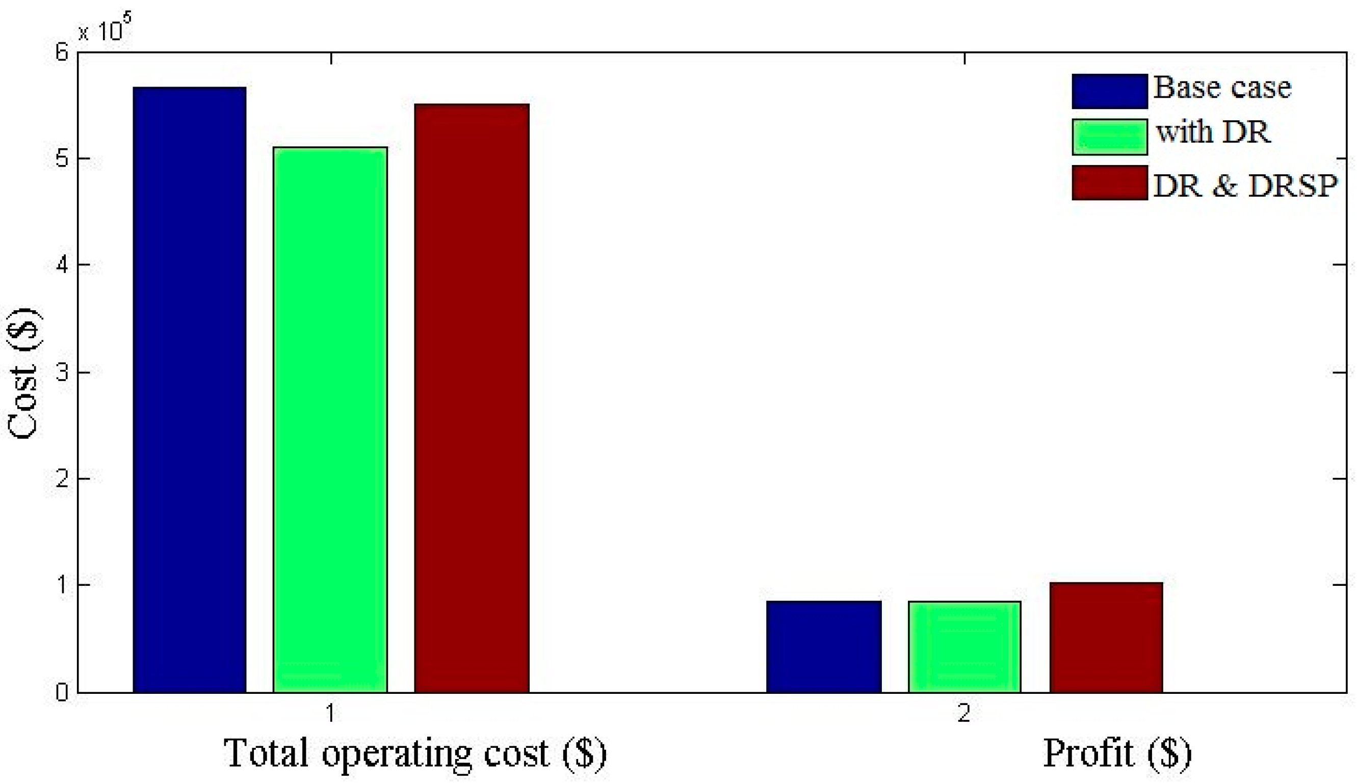
Figure 5.
Unit running data for DRSP switched on during peak hours.
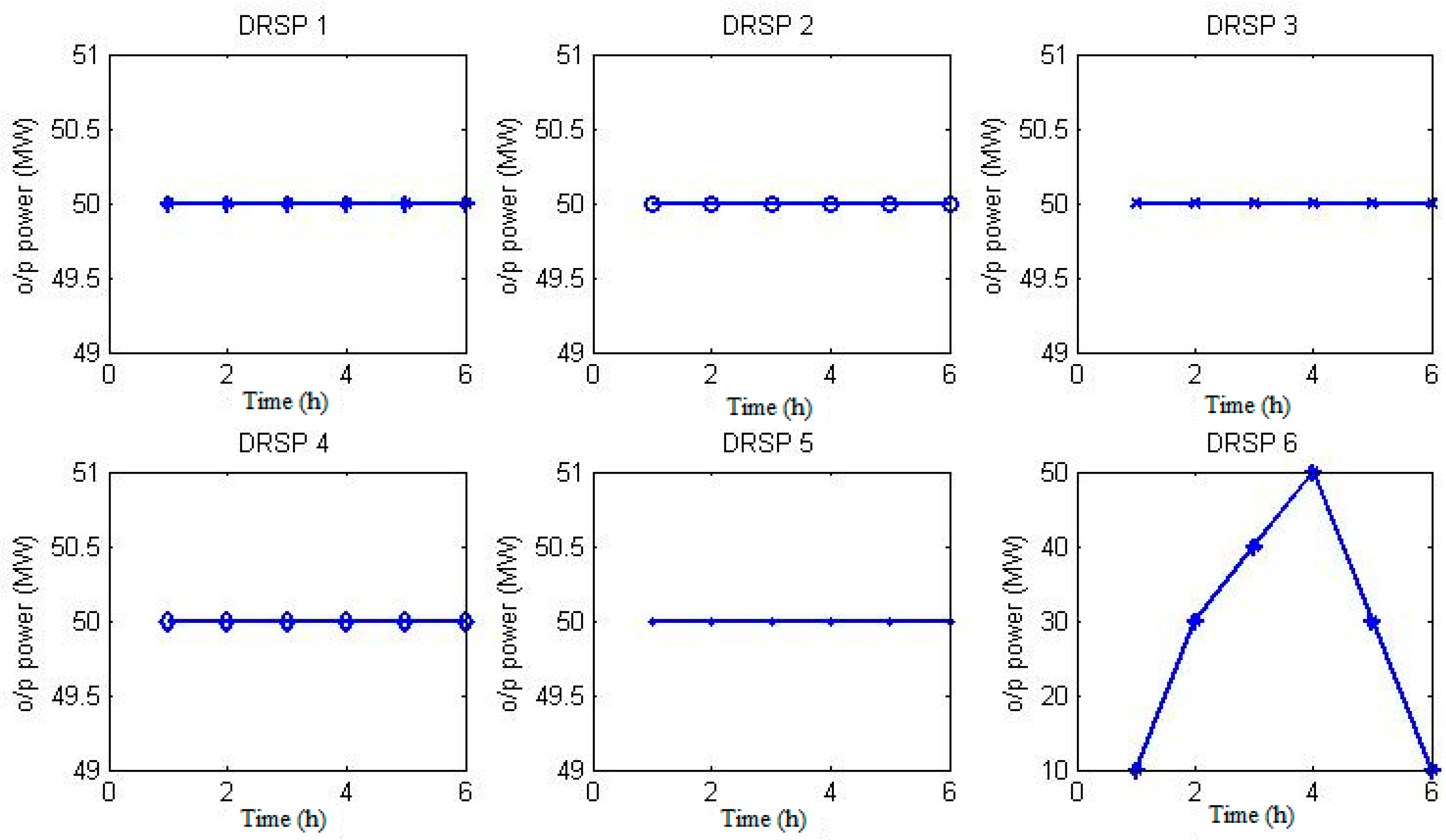
Figure 6.
Load demand vs. time curve for TUC and DRUC.
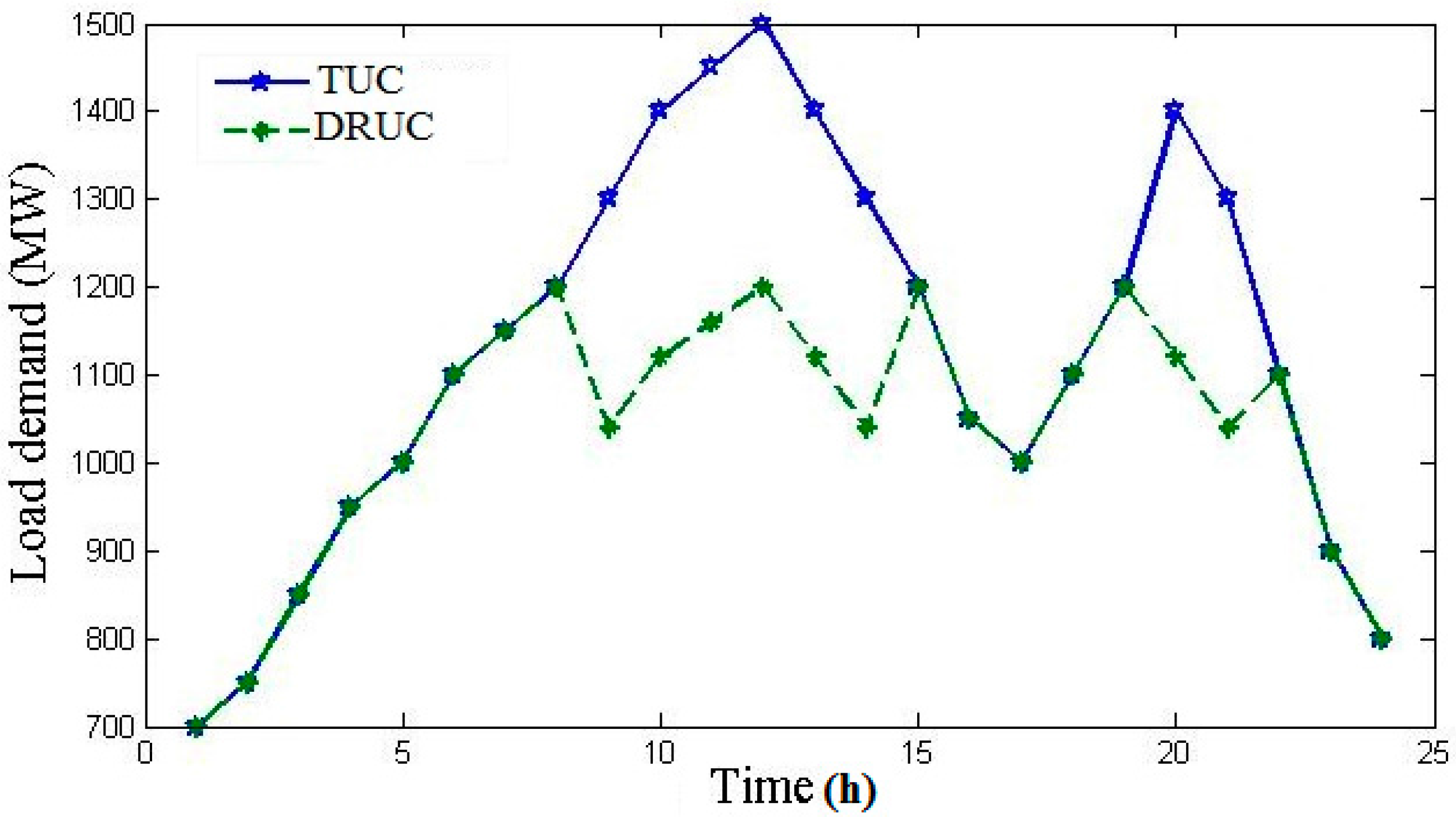
Figure 7.
Profit for TUC, TUC using DR and DRUC.

Figure 8.
Revenue calculated in TUC, TUC using DR and DRUC.
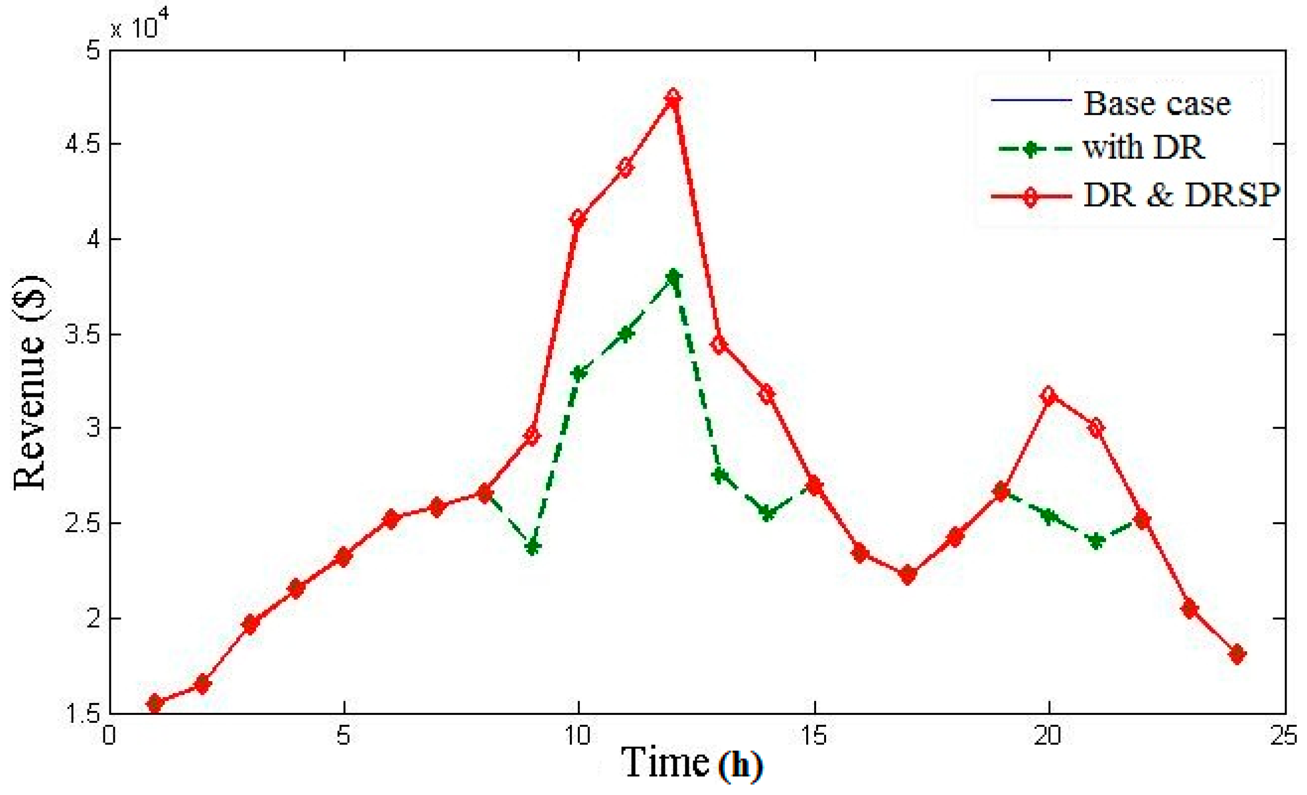
Figure 9.
Operating cost for TUC, TUC using DR and DRUC.


Table 1.
Load curve data for the 10 unit IEEE 39 bus system.
| Unit No. | ai | bi | ci |
|---|---|---|---|
| U-1 | 1000 | 16.19 | 0.00048 |
| U-2 | 970 | 17.26 | 0.00031 |
| U-3 | 700 | 16.6 | 0.002 |
| U-4 | 680 | 16.5 | 0.00211 |
| U-5 | 450 | 19.7 | 0.00398 |
| U-6 | 370 | 22.26 | 0.00712 |
| U-7 | 480 | 27.74 | 0.00079 |
| U-8 | 660 | 25.92 | 0.00413 |
| U-9 | 665 | 27.27 | 0.0022 |
| U-10 | 670 | 27.799 | 0.00173 |
Table 2.
Operator data for the 10 unit IEEE 39 bus system.
| Unit No. | (MW) | (MW) | (h) | (h) | ($) | ($) | (h) | (h) |
|---|---|---|---|---|---|---|---|---|
| U-1 | 455 | 150 | 8 | 8 | 4500 | 9000 | 5 | 8 |
| U-2 | 455 | 150 | 8 | 8 | 5000 | 10,000 | 5 | 8 |
| U-3 | 130 | 20 | 5 | 5 | 550 | 1100 | 4 | −5 |
| U-4 | 130 | 20 | 5 | 5 | 560 | 1120 | 4 | −5 |
| U-5 | 162 | 25 | 6 | 6 | 900 | 1800 | 4 | −6 |
| U-6 | 80 | 20 | 3 | 3 | 170 | 340 | 2 | −3 |
| U-7 | 85 | 25 | 3 | 3 | 260 | 520 | 2 | −3 |
| U-8 | 55 | 10 | 1 | 1 | 30 | 60 | 0 | −1 |
| U-9 | 55 | 10 | 1 | 1 | 30 | 60 | 0 | −1 |
| U-10 | 55 | 10 | 1 | 1 | 30 | 60 | 0 | −1 |
Table 3.
Load demand for 24 h.
| Time (h) | 1 | 2 | 3 | 4 | 5 | 6 | 7 | 8 | 9 | 10 | 11 | 12 |
| Load Demand (MW) | 700 | 750 | 850 | 950 | 1000 | 1100 | 1150 | 1200 | 1300 | 1400 | 1450 | 1500 |
| Time (h) | 13 | 14 | 15 | 16 | 17 | 18 | 19 | 20 | 21 | 22 | 23 | 24 |
| Load Demand (MW) | 1400 | 1300 | 1200 | 1050 | 1000 | 1100 | 1200 | 1400 | 1300 | 1100 | 900 | 800 |
Table 4.
Forecasted price values for 24 h.
| Time (h) | 1 | 2 | 3 | 4 | 5 | 6 | 7 | 8 | 9 | 10 | 11 | 12 |
| Price ($) | 22.15 | 22 | 23.1 | 22.65 | 23.25 | 22.95 | 22.5 | 22.15 | 22.8 | 29.35 | 30.15 | 31.65 |
| Time (h) | 13 | 14 | 15 | 16 | 17 | 18 | 19 | 20 | 21 | 22 | 23 | 24 |
| Price ($) | 24.6 | 24.5 | 22.5 | 22.3 | 22.25 | 22.05 | 22.2 | 22.65 | 23.1 | 22.95 | 22.75 | 22.55 |
Table 5.
Load curve data for DRSP’s.
| - | |||
|---|---|---|---|
| DRSP1 | 0.07 | 70 | 240 |
| DRSP2 | 0.095 | 100 | 200 |
| DRSP3 | 0.09 | 85 | 220 |
| DRSP4 | 0.09 | 110 | 200 |
| DRSP5 | 0.08 | 105 | 220 |
| DRSP6 | 0.075 | 120 | 190 |
Table 6.
Output data for base case using Traditional Unit Commitment (TUC).
| Hour | 1 | 2 | 3 | 4 | 5 | 6 | 7 | 8 | 9 | 10 | Reserve (MW) | ($) | SC ($) | TOcost ($) | ($) | PR ($) |
|---|---|---|---|---|---|---|---|---|---|---|---|---|---|---|---|---|
| 1 | 455 | 245 | 0 | 0 | 0 | 0 | 0 | 0 | 0 | 0 | 210 | 13,683.13 | 0 | 13,683.13 | 15,505 | 1821.87 |
| 2 | 455 | 295 | 0 | 0 | 0 | 0 | 0 | 0 | 0 | 0 | 160 | 14,554.50 | 0 | 14,554.50 | 16,500 | 1945.50 |
| 3 | 455 | 370 | 0 | 0 | 25 | 0 | 0 | 0 | 0 | 0 | 222 | 16,809.45 | 900 | 17,709.45 | 19,635 | 1925.55 |
| 4 | 455 | 455 | 0 | 0 | 40 | 0 | 0 | 0 | 0 | 0 | 122 | 18,597.67 | 0 | 18,597.67 | 21,517.5 | 2919.83 |
| 5 | 455 | 390 | 0 | 130 | 25 | 0 | 0 | 0 | 0 | 0 | 202 | 20,020.02 | 560 | 20,580.02 | 23,250 | 2669.98 |
| 6 | 455 | 360 | 130 | 130 | 25 | 0 | 0 | 0 | 0 | 0 | 232 | 22,387.04 | 1100 | 23,487.04 | 25,245 | 1757.96 |
| 7 | 455 | 410 | 130 | 130 | 25 | 0 | 0 | 0 | 0 | 0 | 182 | 23,261.98 | 0 | 23,261.98 | 25,875 | 2613.02 |
| 8 | 455 | 455 | 130 | 130 | 30 | 0 | 0 | 0 | 0 | 0 | 132 | 24,150.34 | 0 | 24,150.34 | 26,580 | 2429.66 |
| 9 | 455 | 455 | 130 | 130 | 85 | 20 | 25 | 0 | 0 | 0 | 197 | 27,251.06 | 860 | 28,111.06 | 29,640 | 1528.94 |
| 10 | 455 | 455 | 130 | 130 | 162 | 33 | 25 | 10 | 0 | 0 | 152 | 30,057.55 | 60 | 30,117.55 | 41,090 | 10,972.45 |
| 11 | 455 | 455 | 130 | 130 | 162 | 73 | 25 | 10 | 10 | 0 | 157 | 31,916.06 | 60 | 31,976.06 | 43,717.5 | 11,741.44 |
| 12 | 455 | 455 | 130 | 130 | 162 | 80 | 25 | 43 | 10 | 10 | 162 | 33,890.16 | 60 | 33,950.16 | 47,475 | 13,524.84 |
| 13 | 455 | 455 | 130 | 130 | 162 | 33 | 25 | 10 | 0 | 0 | 152 | 30,057.55 | 0 | 30,057.55 | 34,440 | 4382.45 |
| 14 | 455 | 455 | 130 | 130 | 85 | 20 | 25 | 0 | 0 | 0 | 197 | 27,251.06 | 0 | 27,251.06 | 31,850 | 4598.94 |
| 15 | 455 | 455 | 130 | 130 | 30 | 0 | 0 | 0 | 0 | 0 | 132 | 24,150.34 | 0 | 24,150.34 | 27,000 | 2849.66 |
| 16 | 455 | 310 | 130 | 130 | 25 | 0 | 0 | 0 | 0 | 0 | 282 | 21,513.66 | 0 | 21,513.66 | 23,415 | 1901.34 |
| 17 | 455 | 260 | 130 | 130 | 25 | 0 | 0 | 0 | 0 | 0 | 332 | 20,641.82 | 0 | 20,641.82 | 22,250 | 1608.18 |
| 18 | 455 | 360 | 130 | 130 | 25 | 0 | 0 | 0 | 0 | 0 | 232 | 22,387.04 | 0 | 22,387.04 | 24,255 | 1867.96 |
| 19 | 455 | 455 | 130 | 130 | 30 | 0 | 0 | 0 | 0 | 0 | 132 | 24,150.34 | 0 | 24,150.34 | 26,640 | 2489.66 |
| 20 | 455 | 455 | 130 | 130 | 162 | 33 | 25 | 10 | 0 | 0 | 152 | 30,057.55 | 490 | 30,547.55 | 31,710 | 1162.45 |
| 21 | 455 | 455 | 130 | 130 | 85 | 20 | 25 | 0 | 0 | 0 | 197 | 27,251.06 | 0 | 27,251.06 | 30,030 | 2778.94 |
| 22 | 455 | 455 | 0 | 0 | 145 | 20 | 25 | 0 | 0 | 0 | 137 | 22,735.52 | 0 | 22,735.52 | 25,245 | 2509.48 |
| 23 | 455 | 425 | 0 | 0 | 0 | 20 | 0 | 0 | 0 | 0 | 90 | 17,645.36 | 0 | 17,645.36 | 20,475 | 2829.64 |
| 24 | 455 | 345 | 0 | 0 | 0 | 0 | 0 | 0 | 0 | 0 | 110 | 15,427.42 | 0 | 15,427.42 | 18,040 | 2612.58 |
| TOTAL COST ($) | 55,9847.7 | 4090 | 563,937.7 | 651,380 | 87,442.31 | |||||||||||
Table 7.
Output data for base case established with Demand Response (DR) using Demand Response Unit Commitment (DRUC).
Table 7.
Output data for base case established with Demand Response (DR) using Demand Response Unit Commitment (DRUC).
| Hour | 1 | 2 | 3 | 4 | 5 | 6 | 7 | 8 | 9 | 10 | Reserve (MW) | ($) | SC ($) | TOcost ($) | ($) | PR ($) |
|---|---|---|---|---|---|---|---|---|---|---|---|---|---|---|---|---|
| 1 | 455 | 245 | 0 | 0 | 0 | 0 | 0 | 0 | 0 | 0 | 210 | 13,683.13 | 0 | 13,683.13 | 15,505 | 1821.87 |
| 2 | 455 | 295 | 0 | 0 | 0 | 0 | 0 | 0 | 0 | 0 | 160 | 14,554.49 | 0 | 14,554.5 | 16,500 | 1945.5 |
| 3 | 455 | 370 | 0 | 0 | 25 | 0 | 0 | 0 | 0 | 0 | 222 | 16,809.45 | 900 | 17,709.45 | 19,635 | 1925.55 |
| 4 | 455 | 455 | 0 | 0 | 40 | 0 | 0 | 0 | 0 | 0 | 122 | 18,597.67 | 0 | 18,597.67 | 21,517.5 | 2919.83 |
| 5 | 455 | 390 | 0 | 130 | 25 | 0 | 0 | 0 | 0 | 0 | 202 | 20,020.02 | 560 | 20,580.02 | 23,250 | 2669.98 |
| 6 | 455 | 360 | 130 | 130 | 25 | 0 | 0 | 0 | 0 | 0 | 232 | 22,387.04 | 1100 | 23,487.04 | 25,245 | 1757.95 |
| 7 | 455 | 410 | 130 | 130 | 25 | 0 | 0 | 0 | 0 | 0 | 182 | 23,261.98 | 0 | 23,261.98 | 25,875 | 2613.02 |
| 8 | 455 | 455 | 130 | 130 | 30 | 0 | 0 | 0 | 0 | 0 | 132 | 24,150.34 | 0 | 24,150.34 | 26,580 | 2429.66 |
| 9 | 405 | 360 | 130 | 120 | 25 | 0 | 0 | 0 | 0 | 0 | 292 | 21,386.63 | 0 | 21,386.63 | 23,712 | 2325.37 |
| 10 | 455 | 380 | 130 | 130 | 25 | 0 | 0 | 0 | 0 | 0 | 212 | 22,736.83 | 0 | 22,736.83 | 32,872 | 10,135.17 |
| 11 | 455 | 395 | 130 | 130 | 25 | 0 | 25 | 0 | 0 | 0 | 257 | 24,173.33 | 520 | 24,693.33 | 34,974 | 10,280.67 |
| 12 | 455 | 435 | 130 | 130 | 25 | 0 | 25 | 0 | 0 | 0 | 217 | 24,874.02 | 0 | 24,874.02 | 37,980 | 13,105.98 |
| 13 | 455 | 355 | 130 | 130 | 25 | 0 | 25 | 0 | 0 | 0 | 297 | 23,473.63 | 0 | 23,473.63 | 27,552 | 4078.37 |
| 14 | 410 | 355 | 130 | 120 | 25 | 0 | 0 | 0 | 0 | 0 | 292 | 21,382.13 | 0 | 21,382.13 | 25,480 | 4097.87 |
| 15 | 455 | 435 | 130 | 130 | 50 | 0 | 0 | 0 | 0 | 0 | 132 | 24,199.99 | 0 | 24,199.99 | 27,000 | 2800.01 |
| 16 | 415 | 350 | 130 | 130 | 25 | 0 | 0 | 0 | 0 | 0 | 282 | 21,547.94 | 0 | 21,547.94 | 23,415 | 1867.06 |
| 17 | 455 | 260 | 130 | 130 | 25 | 0 | 0 | 0 | 0 | 0 | 332 | 20,641.82 | 0 | 20,641.82 | 22,250 | 1608.18 |
| 18 | 455 | 350 | 130 | 130 | 35 | 0 | 0 | 0 | 0 | 0 | 232 | 22,411.63 | 0 | 22,411.63 | 24,255 | 1843.37 |
| 19 | 455 | 445 | 130 | 130 | 40 | 0 | 0 | 0 | 0 | 0 | 132 | 24,174.74 | 0 | 24,174.74 | 26,640 | 2465.26 |
| 20 | 455 | 380 | 130 | 130 | 25 | 0 | 0 | 0 | 0 | 0 | 212 | 22,736.83 | 0 | 22,736.83 | 25,368 | 2631.17 |
| 21 | 415 | 360 | 110 | 110 | 25 | 20 | 0 | 0 | 0 | 0 | 372 | 21,859.06 | 340 | 22,199.06 | 24,024 | 1824.94 |
| 22 | 455 | 445 | 0 | 120 | 35 | 45 | 0 | 0 | 0 | 0 | 182 | 22,398.79 | 0 | 22,398.79 | 25,245 | 2846.21 |
| 23 | 455 | 425 | 0 | 0 | 0 | 20 | 0 | 0 | 0 | 0 | 90 | 17,645.36 | 0 | 17,645.36 | 20,475 | 2829.64 |
| 24 | 455 | 345 | 0 | 0 | 0 | 0 | 0 | 0 | 0 | 0 | 110 | 15,427.42 | 0 | 15,427.42 | 18,040 | 2612.58 |
| TOTAL COST ($) | 504,534.29 | 3420 | 507,954.3 | 593,389.5 | 85,435.21 | |||||||||||
Table 8.
Output data of DRSP’s during peak hours.
| Hour | DRSP 1 | DRSP 2 | DRSP 3 | DRSP 4 | DRSP 5 | DRSP 6 | Reserve (MW) | ($) | ($) | |
|---|---|---|---|---|---|---|---|---|---|---|
| 9 | 50 | 50 | 50 | 50 | 50 | 10 | 40 | 4810 | 5928 | 1118 |
| 10 | 50 | 50 | 50 | 50 | 50 | 30 | 20 | 5110 | 8218 | 3108 |
| 11 | 50 | 50 | 50 | 50 | 50 | 40 | 10 | 5282.5 | 8743.5 | 3461 |
| 12 | 50 | 50 | 50 | 50 | 50 | 50 | 0 | 5470 | 9495 | 4025 |
| 13 | 50 | 50 | 50 | 50 | 50 | 30 | 20 | 5110 | 6888 | 1778 |
| 14 | 50 | 50 | 50 | 50 | 50 | 10 | 40 | 4810 | 6370 | 1560 |
| 20 | 50 | 50 | 50 | 50 | 50 | 30 | 20 | 5110 | 6342 | 1232 |
| 21 | 50 | 50 | 50 | 50 | 50 | 10 | 40 | 4810 | 6006 | 1196 |
| TOTAL COST ($) | 40,512.5 | 57,990.5 | 17,478 | |||||||
Table 9.
Various data comparisons.
| - | ($) | SC ($) | TOcost ($) | ($) | PR ($) | % Rise |
|---|---|---|---|---|---|---|
| TUC (LR) [45] | - | - | 565,825 | 651,380 | 85,555 | 13.13 |
| TUC (BCGA) [46] | - | - | 567,367 | 651,380 | 84,013 | 12.89 |
| TUC (ICGA) [46] | - | - | 566,404 | 651,380 | 84,976 | 13.05 |
| TUC (BFA) [47] | - | - | 565,872 | 651,380 | 85,508 | 13.13 |
| TUC (ICA) [48] | - | - | 563,938 | 651,380 | 87,442 | 13.42 |
| TUC (CSO) | 559,847.7 | 4090 | 563,937.7 | 651,380 | 87,442.31 | 13.42 |
| DRUC | 504,534.3 | 3420 | 507,954.3 | 593,389.5 | 85,435.21 | 14.40 |
| DRSP | - | - | 40,512.5 | 57,990.5 | 17,478 | 30.14 |
| DRUC + DRSP | - | - | 548,466.8 | 651,380 | 102,913.2 | 15.80 |
| % Difference | Total cost variation = 2.74% | Total profit variation = 2.37% | ||||
© 2017 by the authors. Licensee MDPI, Basel, Switzerland. This article is an open access article distributed under the terms and conditions of the Creative Commons Attribution (CC BY) license (http://creativecommons.org/licenses/by/4.0/).
Share and Cite
MDPI and ACS Style
Selvakumar, K.; Vijayakumar, K.; Boopathi, C.S. Demand Response Unit Commitment Problem Solution for Maximizing Generating Companies’ Profit. Energies 2017, 10, 1465. https://doi.org/10.3390/en10101465
AMA Style
Selvakumar K, Vijayakumar K, Boopathi CS. Demand Response Unit Commitment Problem Solution for Maximizing Generating Companies’ Profit. Energies. 2017; 10(10):1465. https://doi.org/10.3390/en10101465
Chicago/Turabian StyleSelvakumar, K., K. Vijayakumar, and C. S. Boopathi. 2017. "Demand Response Unit Commitment Problem Solution for Maximizing Generating Companies’ Profit" Energies 10, no. 10: 1465. https://doi.org/10.3390/en10101465
Note that from the first issue of 2016, this journal uses article numbers instead of page numbers. See further details here.