Designing a Model for the Global Energy System—GENeSYS-MOD: An Application of the Open-Source Energy Modeling System (OSeMOSYS)

 ,
,  ,
,
Abstract
:1. Introduction
2. GENeSYS-MOD: Model Description
2.1. The Model
2.1.1. Objective Function
2.1.2. Costs
2.1.3. Storage
2.1.4. Transportation
2.1.5. Trade
3. Model Application and Implementation
3.1. Regional Disaggregation and Trade
3.2. Demand and Fuel Disaggregation
3.3. Modeling Period and Investment Restrictions
3.4. Time Disaggregation
3.5. Emissions
3.6. Storage
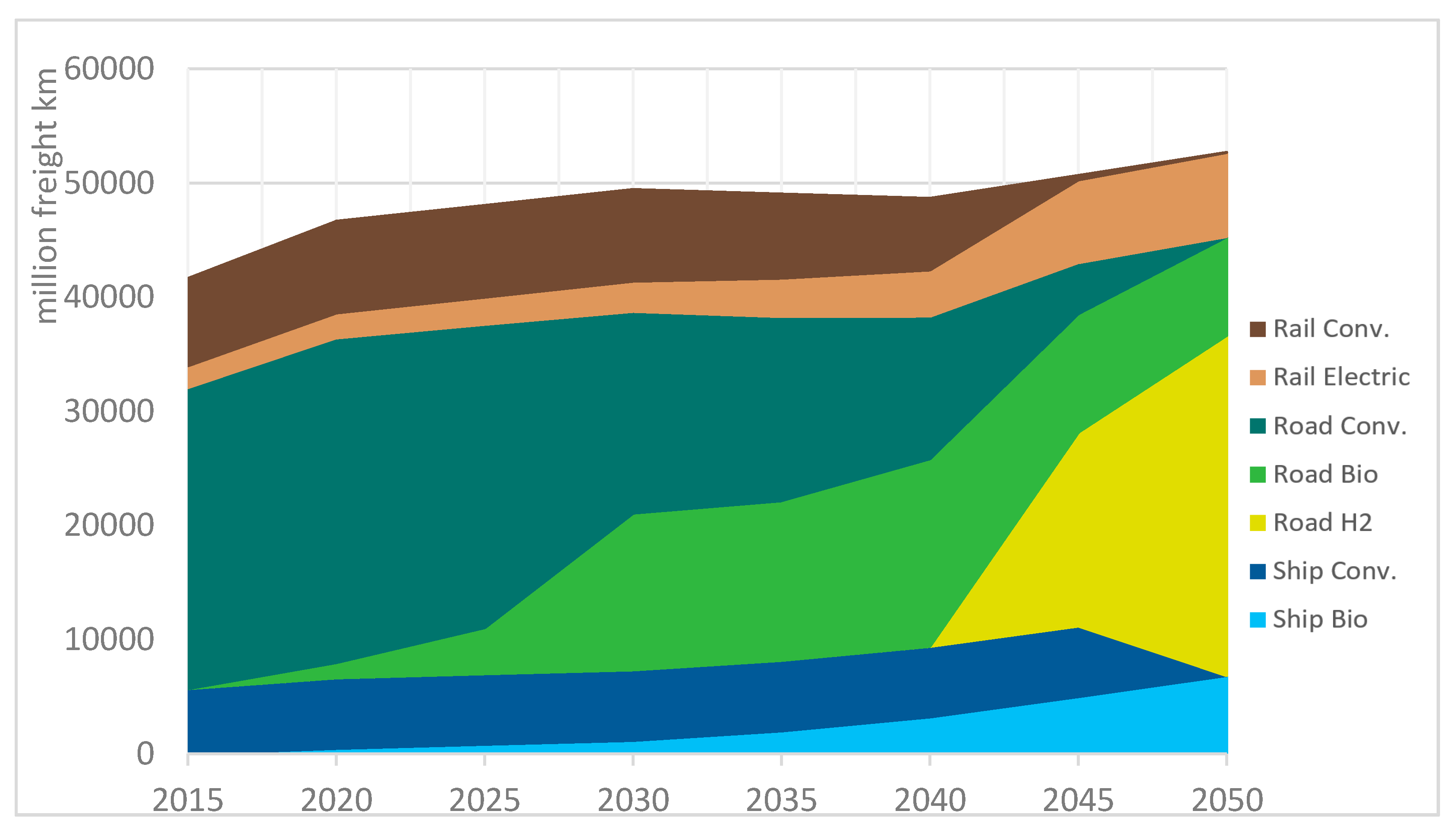
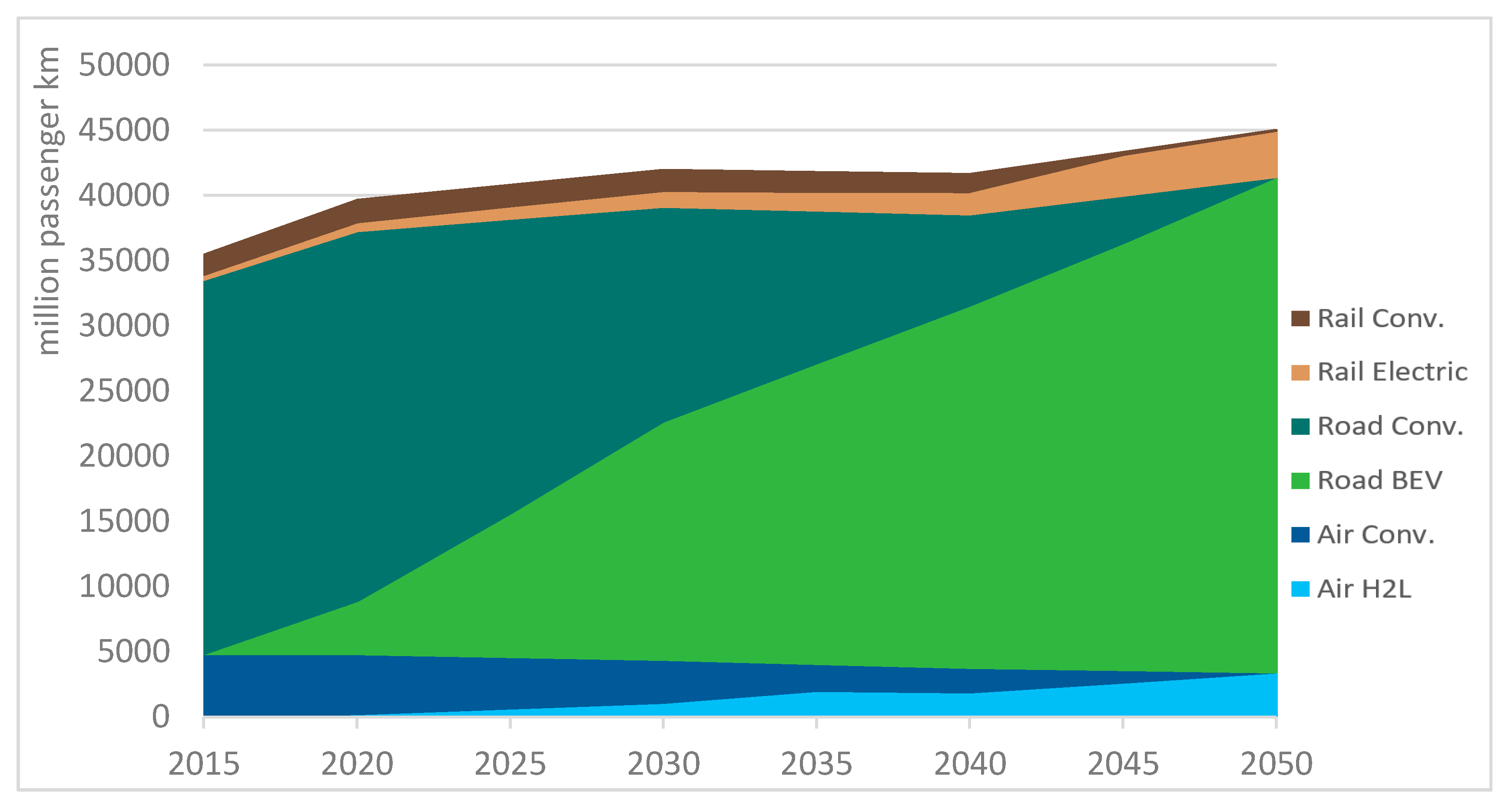
3.7. Modal Split for Transportion
3.8. Input Data
3.8.1. Fossil Fuel Availability and Prices
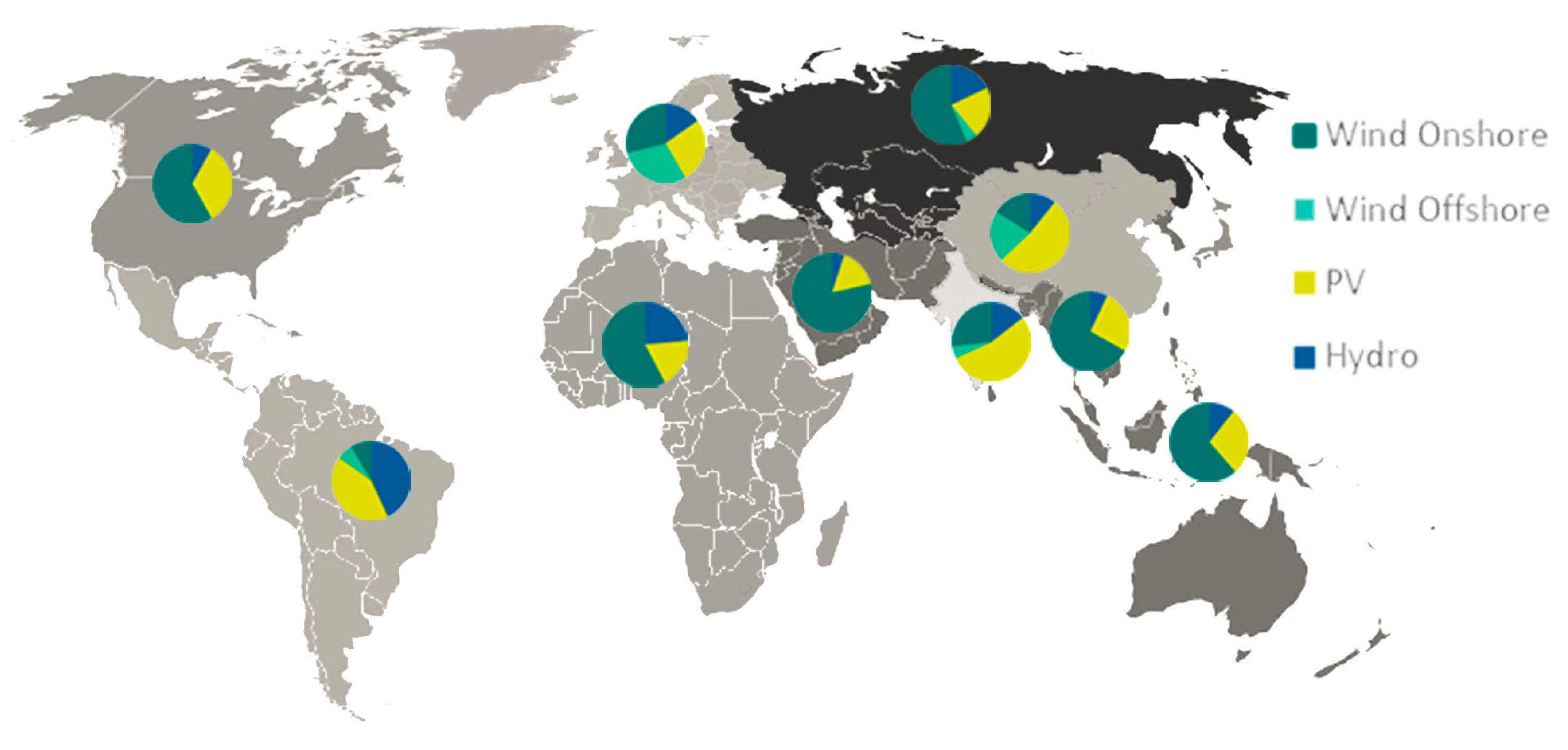
3.8.2. Renewable Technologies and Potentials
3.9. Cost Assumptions
4. Scenario Definition and Results
4.1. Scenario Definition
4.2. Results
4.2.1. The Global Energy System
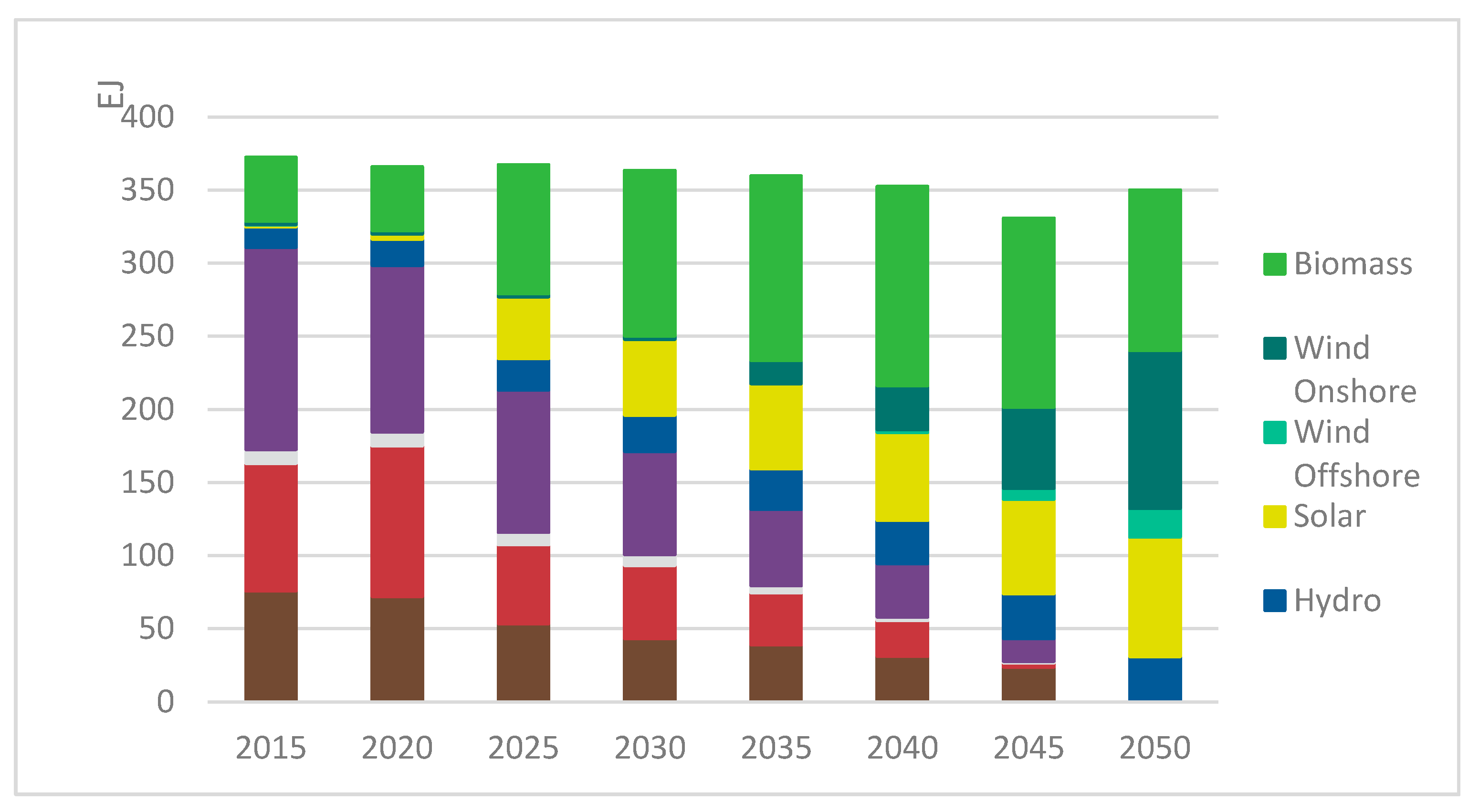
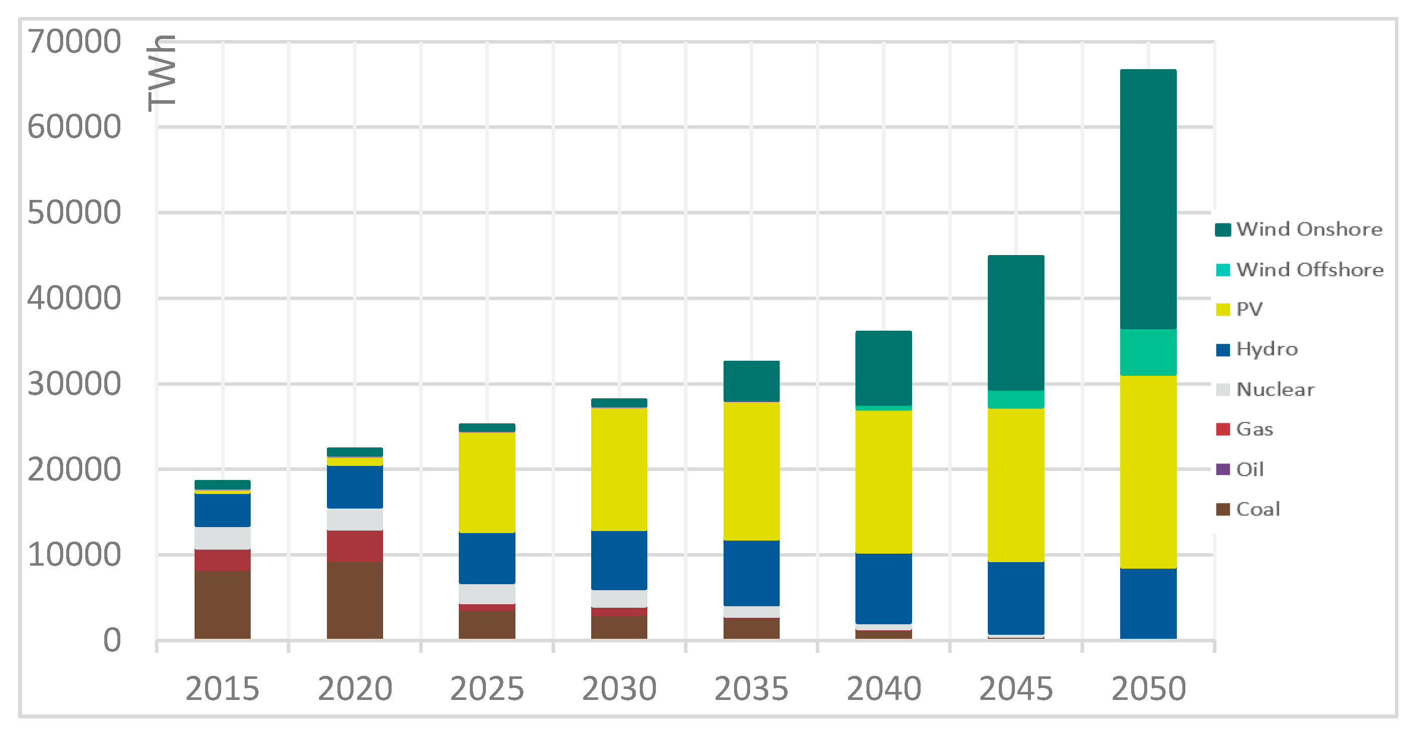
4.2.2. Electricity
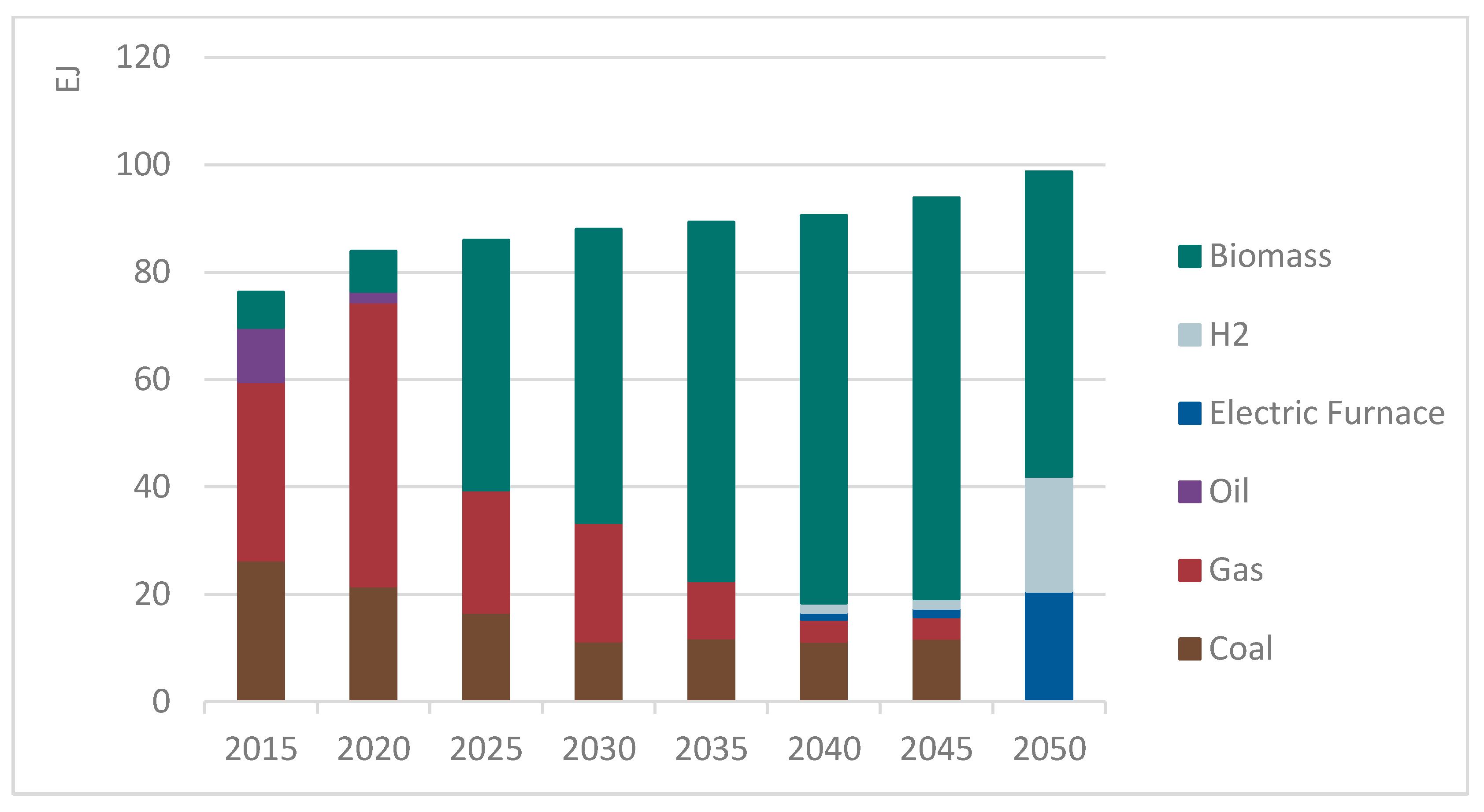
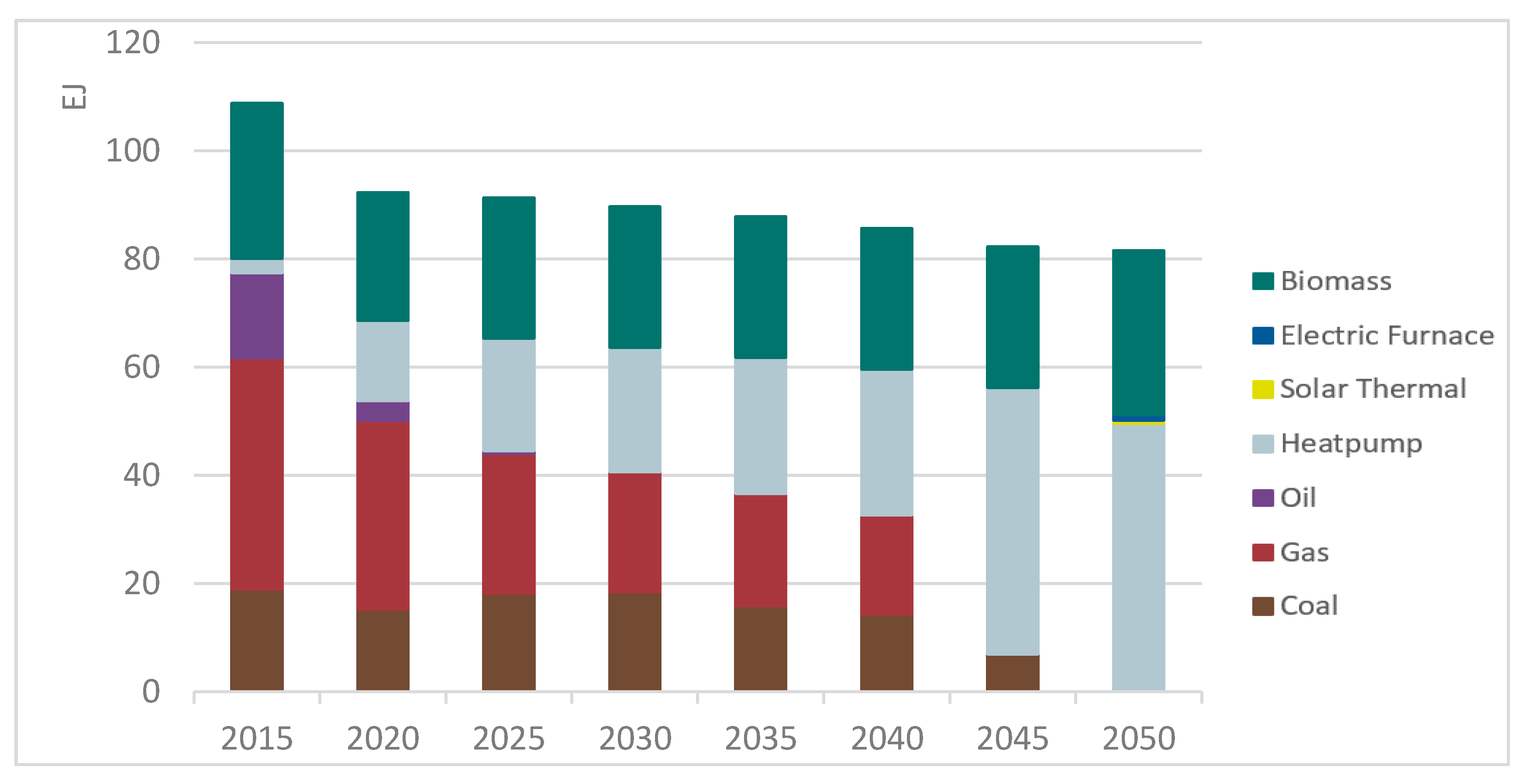
4.2.3. Heat
4.2.4. Transportation
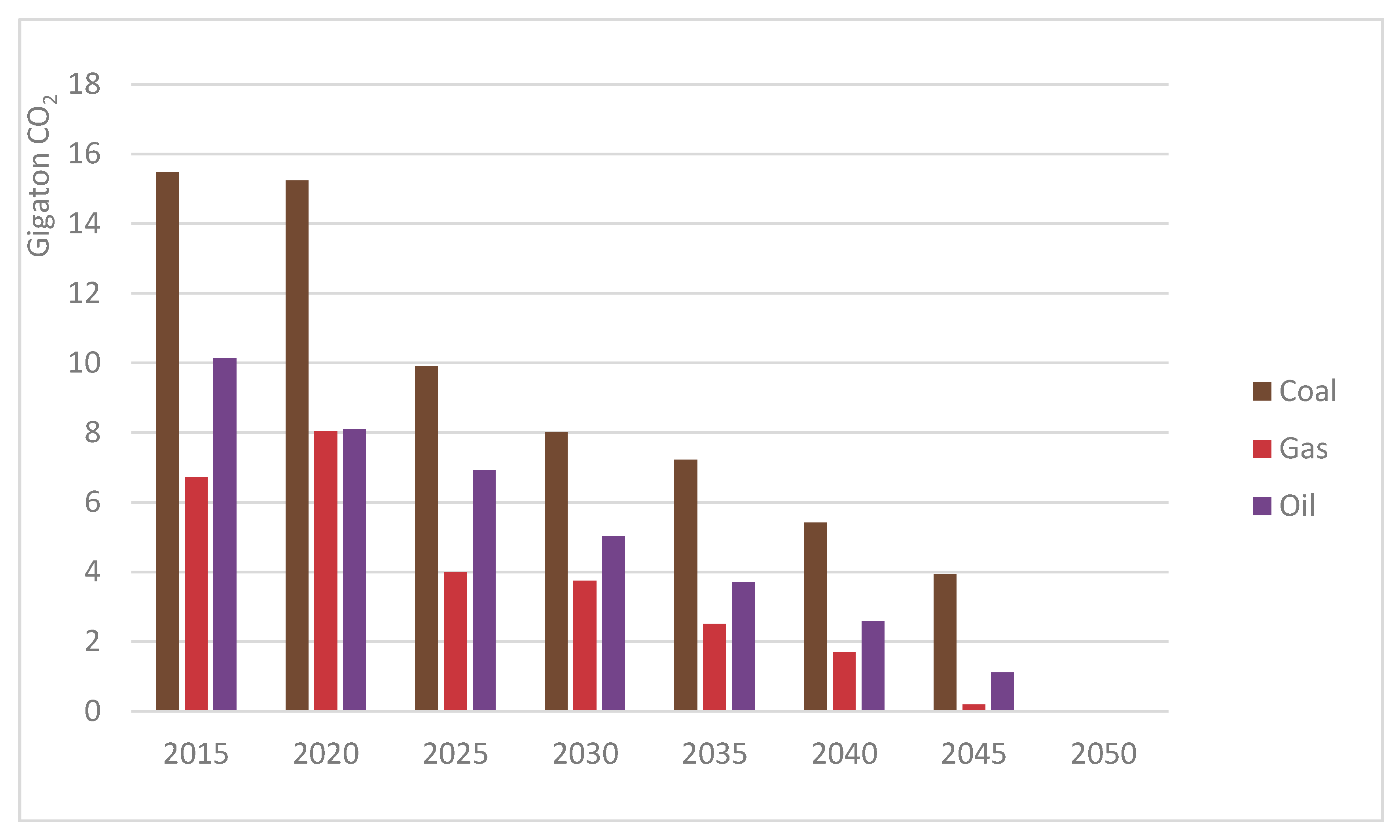
4.2.5 Global CO2 Emissions
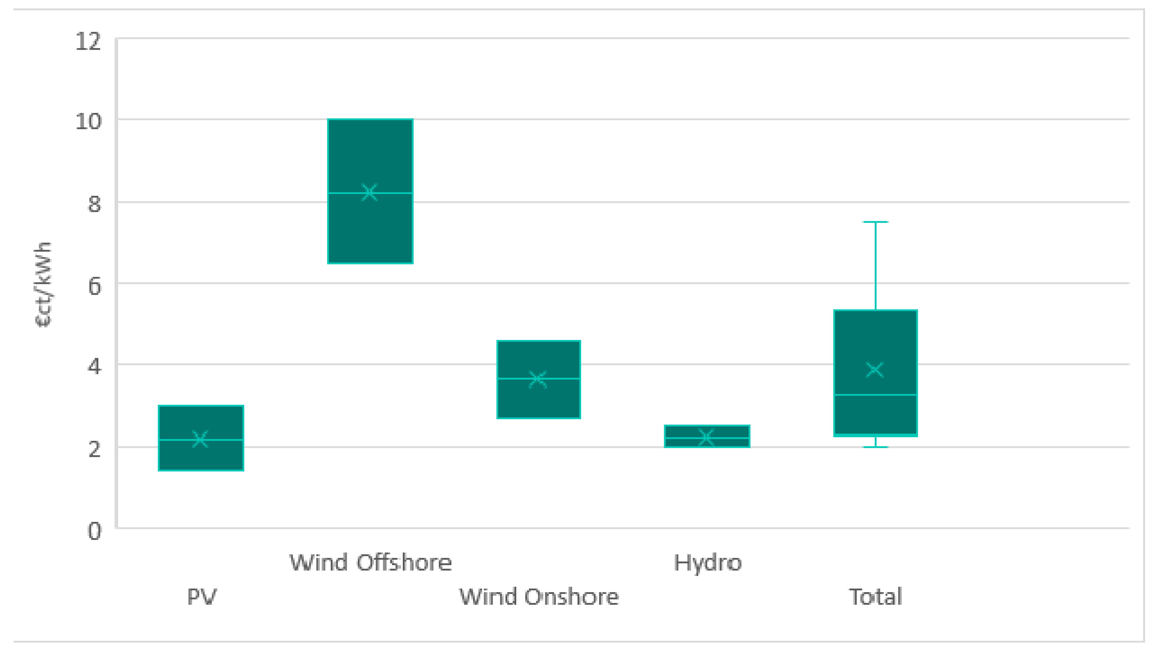
4.2.6. Average Costs
5. Conclusions
Acknowledgments
Author Contributions
Conflicts of Interest
Appendix A
Appendix A.1. List of Sets and Parameters
| Set Name (Abbreviation) | Set Description |
| Daylytimebracket (lh) | Allows for day/night differentiation, i.e., splits a single day into brackets |
| Daytype (ld) | Allows to model different days like weekday/weekend |
| Emissions (e) | Emissions produced by the different technologies |
| Fuel (f) | Fuels enter or leave technologies. Demands are always for specific fuels. |
| Modaltype (mt) | Allows for the modal split in the transportation sector. |
| Mode of Operation (m) | Technologies might operate in different modes, enabling different input-output combinations |
| Region (r) | The different (aggregated) regions considered. |
| Season (ls) | Allows a differentiation for yearly seasons (e.g., summer/winter). |
| Storage (s) | The set of different storage technologies. |
| Technology (t) | Everything that processes energy in any form is considered a technology. |
| Timeslice (l) | Timeslices are a combination of ls, ld and lh. Hence, one timeslice could be “summer weekend day”. |
| Year (y) | The set of the different modeled years. |
| Parameter Name | Parameter Description |
| Amount of demand that can be satisfied at any time of the year, not time-slice dependent. | |
| Amount of emissions allowed in a year and region. | |
| Amount of emissions not produced by modeled technologies in a given year. | |
| Maximum time a technology may run in a year. | |
| Maximum time a technology may run in a time-slice. | |
| Conversion factor of capacities [GW] into activity [PJ]. Assumes provision of 1 [GW] over one year. | |
| Capital costs for storage technologies. | |
| Capital cost for all technologies. | |
| Assigns DailyTimeBracket to time-slice. | |
| Assigns DayType to time-slice. | |
| Assigns Season to time-slice. | |
| Length of a DailyTimeBracket in one day as a fraction of the year. | |
| Amount of days per week in which a DayType occurs. | |
| Amount of emissions produced by a technology for producing 1 [PJ] of energy. | |
| Penalty for emitting emissions. | |
| Fixed O&M costs for a technology. | |
| Describes coupled with OutputActivityRatio the efficiency of a technology. | |
| Percentage of storage capacity that must not be deceeded. | |
| Assigns the share of a mean of transportation for one demand fuel. | |
| Amount of emissions that must not be exceeded over the whole modeling period. | |
| Amount of emissions that is not produced by a modeled technology in whole modeling period. | |
| Operational life of storage technologies. | |
| Operational life of all technologies. | |
| Describes coupled with InputActivityRatio the efficiency of a technology. | |
| Tags fuels that do not produce emissions. | |
| Tags technologies that do not produce emissions. | |
| Tags whether more than the actual demand has to be produced of a given fuel. | |
| Tags which technologies can contribute to the reserve margin. | |
| Sets the amount of reserve margin that has to be produced. | |
| Capacities that exist in addition to the endogenously built capacities. | |
| Storage Capacities that exist in addition to the endogenously built capacities. | |
| Annual demand of fuels which are time-slice dependent. | |
| Assigns a share of SpecifiedAnnualDemand to the different time-slices. | |
| Amount of stored energy at the beginning of the modeling period. | |
| Maximum charge amount of a storage within one hour | |
| Maximum discharge amount of a storage within one hour | |
| Assigns different transportation technologies to the modal type. | |
| Technologies that can use a fuel from a storage. | |
| Technologies that can provide a fuel for a storage. | |
| Maximum amount of investments into a technology in a year. | |
| Maximum amount of used capacity in a year. | |
| Minimum amount of investments into a technology in a year. | |
| Minimum amount of used capacity in a year. | |
| Variable costs for trading a fuel between regions. | |
| Tags possible trade routes between regions. | |
| Variable O&M costs for using a technology. | |
| Share of a time-slice in one year. |
Appendix A.2. List of Technologies and Storages
| Technology | Description |
| Area_DistrictHeating_avg | Usable area for centralized heating (average) |
| Area_DistrictHeating_inf | Usable area for centralized heating (inferior) |
| Area_DistrictHeating_opt | Usable area for centralized heating (optimal) |
| Area_PV_Commercial | Usable area for commercial rooftop PV systems |
| Area_Solar_Roof | Usable area for private rooftop PV systems |
| BIOFLREFINERY | Refinery for biomass to biofuel conversion |
| C_Coal | Coal resource node |
| C_Gas | Gas resource node |
| C_Nuclear | Nuclear material resource node |
| C_Oil | Crude oil resource node |
| ELYSER | Hydrogen-producing elyser |
| FRT_Rail_ELC | Freight rail transport; Electric train |
| FRT_Rail_Petro | Freight rail transport; Petro-fueled |
| FRT_Road_Bio | Freight road transport; Biofuels |
| FRT_Road_Conv | Freight road transport; Conventional fuels |
| FRT_Road_H2 | Freight road transport; Hydrogen-based |
| FRT_Ship_Bio | Freight ship transport; Biofuels |
| FRT_Ship_Conv | Freight ship transport; Conventional fuels |
| FUEL_CELL | Fuel cell |
| H2TL | Hydrogen liquefaction |
| P_Coal | Coal-based power plant |
| P_Gas | Natural gas-based power plant |
| P_Nuclear | Nuclear power plant |
| P_Oil | Oil power plant |
| PSNG_Air_Conv | Passenger air transport; Conventional fuels |
| PSNG_Air_H2L | Passenger air transport; Liquid hydrogen |
| PSNG_Rail_ELC | Passenger rail transport; Electric train |
| PSNG_Rail_Petro | Passenger rail transport; Petro-fueled |
| PSNG_Road_BEV | Passenger road transport; Battery electric vehicle |
| PSNG_Road_Bio | Passenger road transport; Biofuels |
| PSNG_Road_FCEV | Passenger road transport; Fuel cell electric vehicle |
| PSNG_Road_ICE | Passenger road transport; Internal combustion engine |
| Res_BioMass | Biomass resource node |
| Res_CSP | Concentrated solar power plant |
| Res_CSP_Storage | Concentrated solar power plant with integrated storage |
| Res_Hydro_Large | Large-scale hydro (>25MW) |
| Res_Hydro_Small | Small-scale hydro |
| Res_PV_Commercial | Rooftop-PV on commercial buildings |
| Res_PV_Residential | Residential rooftop PV systems |
| Res_PV_Utility_avg | Utility-scale PV (average) |
| Res_PV_Utility_inf | Utility-scale PV (inferior) |
| Res_PV_Utility_opt | Utility-scale PV (optimal) |
| Res_Thermal_Geo | Geothermal power generation |
| Res_Thermal_Solar | Solar-based heat generation |
| Res_Tidal | Tidal power plant |
| Res_Wave | Wave power plant |
| Res_Wind_Offshore_avg | Offshore wind plant (average) |
| Res_Wind_Offshore_inf | Offshore wind plant (inferior) |
| Res_Wind_Offshore_opt | Offshore wind plant (optimal) |
| Res_Wind_Onshore_avg | Onshore wind plant (average) |
| Res_Wind_Onshore_inf | Onshore wind plant (inferior) |
| Res_Wind_Onshore_opt | Onshore wind plant (optimal) |
| ST_Battery_Lion | Dummy-Technology for battery storage |
| ST_H2 | Dummy-Technology for hydrogen storage |
| ST_Heat_cen | Dummy-Technology for central heat storage |
| ST_Heat_dec | Dummy-Technology for decentral heat storage |
| ST_PSP | Dummy-Technology for pump storage |
| ST_PSP_Residual | Dummy-Technology for residual pump storage capacities |
| T_heat_high_bio | High-temperature heat generation (biomass) |
| T_heat_high_coal | High-temperature heat generation (coal) |
| T_heat_high_elfur | High-temperature heat generation (electric furnace) |
| T_heat_high_gas | High-temperature heat generation (natural gas) |
| T_heat_high_oil | High-temperature heat generation (oil) |
| T_heat_high_res-gas | High-temperature heat generation (hydrogen) |
| T_heat_low_bio | Low-temperature heat generation (biomass) |
| T_heat_low_bio_cen | Low-temperature heat generation (biomass; centralized) |
| T_heat_low_bio_chp | Low-temperature heat generation (biomass; combined heat-power-plant) |
| T_heat_low_bio_chp_cen | Low-temperature heat generation (biomass; centralized; combined heat-power-plant) |
| T_heat_low_coal | Low-temperature heat generation (coal) |
| T_heat_low_coal_cen | Low-temperature heat generation (coal; centralized) |
| T_heat_low_coal_chp_cen | Low-temperature heat generation (coal; centralized; combined heat-power-plant) |
| T_heat_low_elfur | Low-temperature heat generation (electric furnace) |
| T_heat_low_elfur_cen | Low-temperature heat generation (electric furnace; centralized) |
| T_heat_low_gas | Low-temperature heat generation (natural gas) |
| T_heat_low_gas_cen | Low-temperature heat generation (natural gas; centralized) |
| T_heat_low_gas_chp_cen | Low-temperature heat generation (natural gas; centralized; combined heat-power-plant) |
| T_heat_low_heatpump | Low-temperature heat generation (heatpump) |
| T_heat_low_heatpump_cen | Low-temperature heat generation (heatpump; centralized) |
| T_heat_low_oil | Low-temperature heat generation (oil) |
| T_heat_low_oil_cen | Low-temperature heat generation (oil; centralized) |
| T_heat_low_oil_chp_cen | Low-temperature heat generation (oil; centralized; combined heat-power-plant) |
| T_heat_low_res-gas | Low-temperature heat generation (hydrogen) |
| T_heat_low_res-gas_cen | Low-temperature heat generation (hydrogen; centralized) |
| T_heat_low_res-gas_chp | Low-temperature heat generation (hydrogen; combined-heat-power-plant) |
| T_heat_low_res-gas_chp_cen | Low-temperature heat generation (hydrogen; centralized; combined heat-power-plant) |
| Storages | |
| S_Battery_Lion | Lithium-Ion battery |
| S_CSP_storage | Storage-technology connected to CSP with storage |
| S_H2 | Hydrogen (gas) storage |
| S_Heat_cen | Heat storage for central heating |
| S_Heat_dec | Heat storage for decentral heating |
| S_PSP | (Hydro) Pump-storage-plant |
Appendix A.3. List of Countries, Grouped by Region
| Africa | ||
| Algeria | Ethiopia | Niger |
| Angola | Gabon | Nigeria |
| Benin | Gambia (Islamic Republic of) | Rwanda |
| Botswana | Ghana | Sao Tome and Principe |
| Burkina Faso | Guinea | Senegal |
| Burundi | Guinea Bissau | Sierra Leone |
| Cabo Verde | Kenya | Somalia |
| Cameroon | Lesotho | South Africa |
| Central African Republic | Liberia | South Sudan |
| Chad | Libya | Sudan |
| Comoros | Madagascar | Swaziland |
| Congo | Malawi | Togo |
| Côte D'Ivoire | Mali | Tunisia |
| Democratic Republic of the Congo | Mauritania | Uganda |
| Djibouti | Mauritius | United Republic of Tanzania |
| Egypt | Morocco | Zambia |
| Equatorial Guinea | Mozambique | Zimbabwe |
| Eritrea | Namibia | |
| Asia-Rest | ||
| Bangladesh | Malaysia | Singapore |
| Bhutan | Maldives | Sri Lanka |
| Brunei Darussalam | Myanmar | Thailand |
| Cambodia | Nepal | Timor-Leste |
| Indonesia | Philippines | Viet Nam |
| Lao People’s Democratic Republic | Seychelles | |
| China | ||
| China | Mongolia | |
| Europe | ||
| Albania | Germany | Norway |
| Andorra | Greece | Poland |
| Austria | Hungary | Portugal |
| Belarus | Iceland | Romania |
| Belgium | Ireland | San Marino |
| Bosnia and Herzegovina | Italy | Serbia |
| Bulgaria | Latvia | Slovakia |
| Croatia | Liechtenstein | Slovenia |
| Cyprus | Lithuania | Spain |
| Czech Republic | Luxembourg | Sweden |
| Denmark | Malta | Switzerland |
| Estonia | Monaco | The former Yugoslav Republic of Macedonia |
| Finland | Montenegro | Ukraine |
| France | Netherlands | United Kingdom of Great Britain and Northern Ireland |
| India | ||
| India | ||
| Middle East | ||
| Afghanistan | Kuwait | Syrian Arab Republic |
| Bahrain | Lebanon | Turkey |
| Iran (Islamic Republic of) | Oman | United Arab Emirates |
| Iraq | Pakistan | Yemen |
| Israel | Qatar | |
| Jordan | Saudi Arabia | |
| North America | ||
| Canada | Mexico | United States of America |
| Ocenania | ||
| Australia | Micronesia (Federated States of) | Samoa |
| Democratic People’s Republic of Korea | Nauru | Solomon Islands |
| Fiji | New Zealand | Tonga |
| Japan | Palau | Tuvalu |
| Kiribati | Papua New Guinea | Vanuatu |
| Marshall Islands | Republic of Korea | |
| FSU | ||
| Armenia | Kyrgyzstan | Uzbekistan |
| Azerbaijan | Russian Federation | Republic of Moldova |
| Georgia | Tajikistan | |
| Kazakhstan | Turkmenistan | |
| South America | ||
| Antigua and Barbuda | Dominica | Panama |
| Argentina | Dominican Republic | Paraguay |
| Bahamas | Ecuador | Peru |
| Barbados | El Salvador | Saint Kitts and Nevis |
| Belize | Grenada | Saint Lucia |
| Bolivia (Plurinational State of) | Guatemala | Saint Vincent and the Grenadines |
| Brazil | Guyana | Suriname |
| Chile | Haiti | Trinidad and Tobago |
| Colombia | Honduras | Uruguay |
| Costa Rica | Jamaica | Venezuela, Bolivarian Republic of |
| Cuba | Nicaragua | |
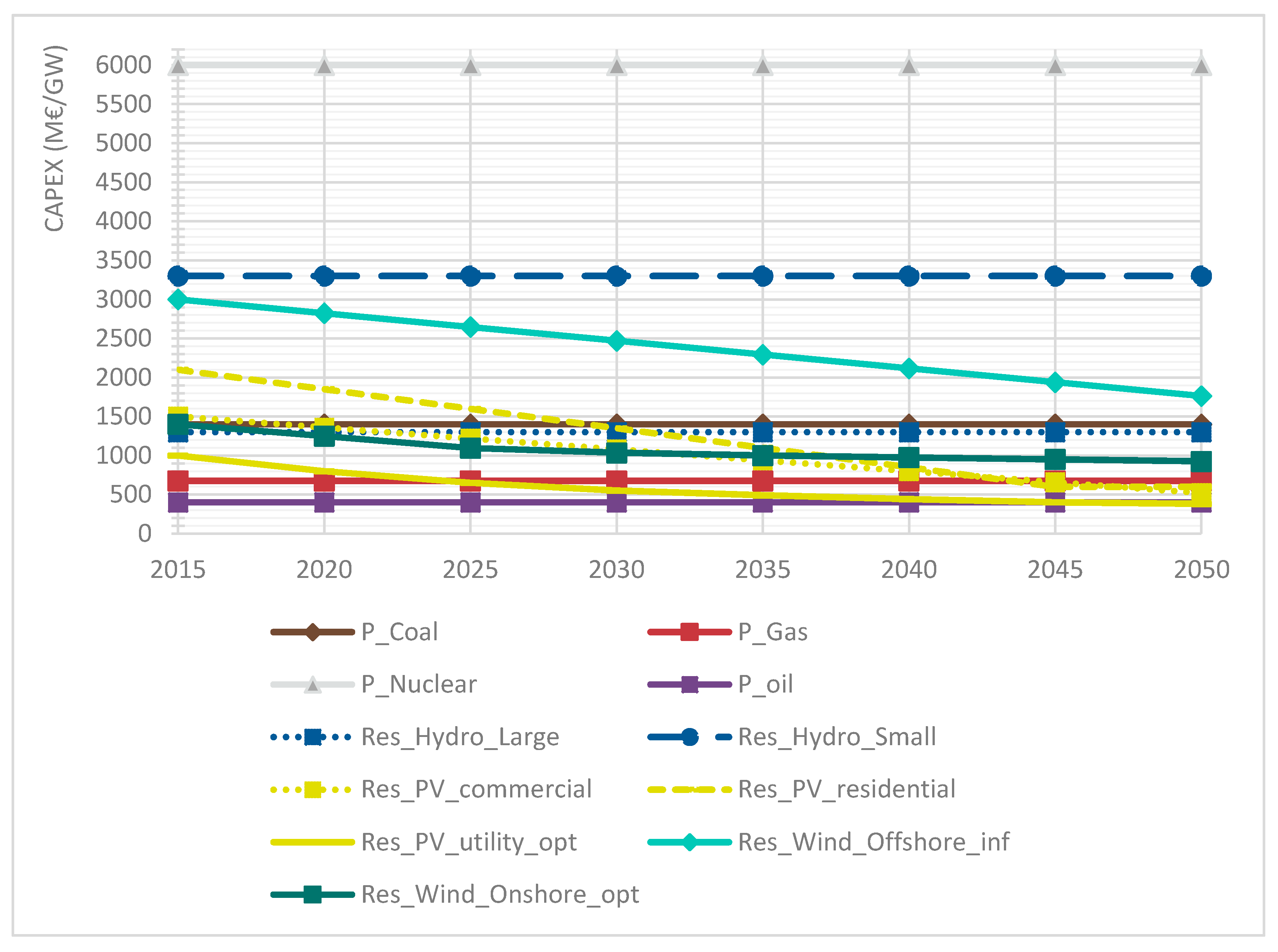
Appendix A.4. Capital Cost Development of Electricity-Generating Technologies (in million €/GW)
References
- Connolly, D.; Lund, H.; Mathiesen, B.V.; Leahy, M. A review of computer tools for analysing the integration of renewable energy into various energy systems. Appl. Energy 2010, 87, 1059–1082. [Google Scholar] [CrossRef]
- Herbst, A.; Toro, F.; Reitze, F.; Jochem, E. Introduction to energy systems modelling. Swiss J. Econ. Stat. 2012, 148, 111–135. [Google Scholar]
- Bhattacharyya, S.C.; Timilsina, G.R. A review of energy system models. Int. J. Energy Sect. Manag. 2010, 4, 494–518. [Google Scholar] [CrossRef]
- Seebregts, A.; Gary, G.; Koen, S. Energy/environmental modeling with the MARKAL family of models. In Operations Research Proceedings 2001; Chamoni, P., Leisten, R., Martin, A., Minnemann, J., Stadtler, H., Eds.; Springer-Verlag: Duisburg, Germany, 2001; Volume 2001, pp. 75–82. ISBN 978-3-540-43344-6. [Google Scholar]
- EIA The National Energy Modeling System: An Overview. Available online: https://www.eia.gov/outlooks/aeo/nems/overview/index.html (accessed on 19 September 2017).
- IIASA MESSAGE. Available online: http://www.iiasa.ac.at/web/home/research/researchPrograms/Energy/MESSAGE.en.html (accessed on 11 July 2017).
- E3MLab. PRIMES Model; E3Mlab, National Technocal University of Athens: Athens, Greece, 2016. [Google Scholar]
- Yang, Z.; Eckaus, R.S.; Ellerman, A.D.; Jacoby, H.D. The MIT Emissions Prediction and Policy Analysis (EPPA) Model; Joint Program on the Science and Policy of Global Change: Cambridge, MA, USA, 1996; p. 49. [Google Scholar]
- Criqui, P. International Markets and Energy Prices: The POLES Model. In Models for Energy Policy; Lesourd, J.-B., Percebois, J., Valette, F., Eds.; Routledge Studies in the History of Economic Modelling; Routledge: Abingdon, UK, 1996; pp. 14–29. ISBN 978-0-415-12975-6. [Google Scholar]
- Mundaca, L.; Neij, L. A multi-criteria evaluation framework for tradable white certificate schemes. Energy Policy 2009, 37, 4557–4573. [Google Scholar] [CrossRef]
- Heaps, C. An introduction to LEAP. Stockh. Environ. Inst. 2008, 1–16. Available online: https://www.energycommunity.org/documents/LEAPIntro.pdf (accessed on 19 September 2017).
- SSRN, Wind Providing Balancing Reserves—An Application to the German Electricity System of 2025. Available online: https://papers.ssrn.com/soL3/papers.cfm?abstract_id=2952288 (accessed on 9 September 2017).
- Clack, C.T.M.; Qvist, S.A.; Apt, J.; Bazilian, M.; Brandt, A.R.; Caldeira, K.; Davis, S.J.; Diakov, V.; Handschy, M.A.; Hines, P.D.H.; et al. Evaluation of a proposal for reliable low-cost grid power with 100% wind, water, and solar. Proc. Natl. Acad. Sci. USA 2017, 114, 6722–6727. [Google Scholar] [CrossRef] [PubMed]
- Jacobson, M.Z.; Delucchi, M.A.; Cameron, M.A.; Frew, B.A. The United States can keep the grid stable at low cost with 100% clean, renewable energy in all sectors despite inaccurate claims. Proc. Natl. Acad. Sci. USA 2017, 114, E5021–E5023. [Google Scholar] [CrossRef] [PubMed]
- Moura, G.; Howells, M.; Legey, L. SAMBA, The open source South American Model Base. A Brazilian Perspective on Long Term Power Systems Investment and Integration; Technical Report; Royal Institute of Technology: Stockholm, Sweden, 2015. [Google Scholar]
- Rogan, F.; Cahill, C.J.; Daly, H.E.; Dineen, D.; Deane, J.P.; Heaps, C.; Welsch, M.; Howells, M.; Bazilian, M.; Gallachóir, B.P.Ó. LEAPs and Bounds—An Energy Demand and Constraint Optimised Model of the Irish Energy System. Energy Effic. 2014, 7, 441–466. [Google Scholar] [CrossRef]
- Lyseng, B.; Rowe, A.; Wild, P.; English, J.; Niet, T.; Pitt, L. Decarbonising the Alberta power system with carbon pricing. Energy Strategy Rev. 2016, 10, 40–52. [Google Scholar] [CrossRef]
- Burandt, T.; Hainsch, K.; Löffler, K.; Böing, H.; Erbe, J.; Kafemann, I.-V.; Kendziorski, M.; Kruckelmann, J.; Rechtlitz, J.; Scherwath, T. Designing a Global Energy System based on 100% Renewables for 2050-Insights from the Open-source Energy Modelling System (OSeMOSYS) 2016. Available online: https://ideas.repec.org/p/diw/diwwpp/dp1678.html (accessed on 9 September 2017).
- Noble, K. OSeMOSYS: The Open Source Energy Modeling System—A Translation into the General Algebraic Modeling System (GAMS); KTH: Stockholm, Sweden, 2012; Available online: http://www.osemosys.org/uploads/1/8/5/0/18504136/osemosys_in_gams_wp_desa_2012.pdf (accessed on 19 September 2017).
- Howells, M.; Rogner, H.; Strachan, N.; Heaps, C.; Huntington, H.; Kypreos, S.; Hughes, A.; Silveira, S.; DeCarolis, J.; Bazillian, M.; et al. OSeMOSYS: The Open Source Energy Modeling System: An introduction to its ethos, structure and development. Energy Policy 2011, 39, 5850–5870. [Google Scholar] [CrossRef]
- Welsch, M.; Howells, M.; Bazilian, M.; DeCarolis, J.F.; Hermann, S.; Rogner, H.H. Modelling elements of Smart Grids–Enhancing the OSeMOSYS (Open Source Energy Modelling System) code. Energy 2012, 46, 337–350. [Google Scholar] [CrossRef]
- Intergovernmental Panel on Climate Change (IPCC). Summary for Policymakers. In Climate Change 2014: Impacts, Adaptation, and Vulnerability. Part A: Global and Sectoral Aspects. Contribution of Working Group II to the Fifth Assessment Report of the Intergovernmental Panel on Climate Change; Cambridge University Press: Cambridge, NY, USA, 2014. [Google Scholar]
- NEI Comparison of Lifecycle Emissions of Energy Technologies. Available online: http://www.nei.org/Issues-Policy/Protecting-the-Environment/Life-Cycle-Emissions-Analyses/Comparison-of-Lifecycle-Emissions-of-Selected-Ener (accessed on 19 September 2017).
- Renewable Energy Sources and Climate Change Mitigation: Special Report of the Intergovernmental Panel on Climate Change; Edenhofer, O.; Pichs Madruga, R.; Sokona, Y.; UNEP; WMO; IPCC; PIK (Eds.) Cambridge University Press: Cambridge, NY, USA, 2012; ISBN 978-1-107-02340-6. [Google Scholar]
- EIA International Energy Outlook 2016. Available online: https://www.eia.gov/outlooks/ieo/pdf/0484(2016).pdf (accessed on 19 September 2017).
- World Energy Outlook 2015; International Energy Agency (Ed.) OECD: Paris, France, 2015; ISBN 978-92-64-24365-1. Available online: http://www.worldenergyoutlook.org/media/weowebsite/2015/WEO2015_Chapter01.pdf (accessed on 19 September 2017).
- Farfan, J.; Breyer, C. Structural changes of global power generation capacity towards sustainability and the risk of stranded investments supported by a sustainability indicator. J. Clean. Prod. 2017, 141, 370–384. [Google Scholar] [CrossRef]
- OECD, Renewables Information 2016. Available online: http://www.oecd-ilibrary.org/energy/renewables-information-2016_renew-2016-en;jsessionid=lxmv0jej2xlb.x-oecd-live-03 (accessed on 22 September 2017).
- Jacobson, M.Z.; Delucchi, M.A.; Bauer, Z.A.F.; Goodman, S.C.; Chapman, W.E.; Cameron, M.A.; Bozonnat, C.; Chobadi, L.; Clonts, H.A.; Enevoldsen, P.; et al. 100% Clean and Renewable Wind, Water, and Sunlight All-Sector Energy Roadmaps for 139 Countries of the World. Joule 2017, 108–121. [Google Scholar] [CrossRef]
- Trieb, F.; Schillings, C.; O’Sullivan, M.; Pregger, T.; Hoyer-Klick, C. Global Potential of Concentrating Solar Power. In Proceedings of the SolarPaces Conference, Berlin, Germany, 15–18 September 2009. [Google Scholar]
- Archer, C.L.; Jacobson, M. Evaluation of global wind power. J. Geophys. Res. 2005, 110. [Google Scholar] [CrossRef]
- Marvel, K.; Kravitz, B.; Caldeira, K. Geophysical limits to global wind power. Nat. Clim. Chang. 2012, 3, 118–121. [Google Scholar] [CrossRef]
- Hau, E. Windkraftanlagen; Springer: Berlin/Heidelberg, Germany, 2008; ISBN 978-3-540-72150-5. [Google Scholar]
- Schröder, A.; Kunz, F.; Meiss, J.; Mendelevitch, R.; Hirschhausen, C. Current and Prospective Costs of Electricity Generation until 2050; DIW: Berlin, Germany, 2013.
- Arent, D.; Sullivan, P.; Heimiller, D.; Lopez, A.; Eurek, K.; Badger, J.; Jorgensen, H.E.; Kelly, M. Improved Offshore Wind Resource Assessment in Global Climate Stabilization Scenarios; Technical Report; NREL: Golden, CO, USA, 2012; p. 24.
- Sims, R.E.H.; Mabee, W.; Saddler, J.N.; Taylor, M. An overview of second generation biofuel technologies. Bioresour. Technol. 2010, 101, 1570–1580. [Google Scholar] [CrossRef] [PubMed]
- Mühlenh, J. Reststoffe Für Bioenergie Nutzen-Potenziale, Mobilisierung Und Umweltbilanz; Agentur für Erneuerbare Energien: Berlin, Germany, 2013; p. 45. [Google Scholar]
- Gustavsson, J. Global Food Losses and Food Waste: Extent, Causes and Prevention: Study Conducted for the International Congress “Save Food!”; Technical Report; Food and Agriculture Organization of the United Nations: Rome, Italy, 2011; ISBN 978-92-5-107205-9. [Google Scholar]
- International Energy Agency (IEA). Energy Technology Perspectives 2016-Towards Sustainable Urban Energy Systems; International Energy Agency (IEA): Paris, France, 2016; ISBN 978-92-64-25233-2. [Google Scholar]
- Havlík, P.; Schneider, U.A.; Schmid, E.; Böttcher, H.; Fritz, S.; Skalský, R.; Aoki, K.; Cara, S.D.; Kindermann, G.; Kraxner, F.; et al. Global land-use implications of first and second generation biofuel targets. Energy Policy 2011, 39, 5690–5702. [Google Scholar] [CrossRef]
- Handbook of Energy. Vol. 1: Diagrams, Charts, and Tables; Cleveland, C.J.; Morris, C. (Eds.) Elsevier: Amsterdam, The Netherlands, 2013; ISBN 978-0-08-046405-3. [Google Scholar]
- Younger, P. Geothermal Energy: Delivering on the Global Potential. Energies 2015, 8, 11737–11754. [Google Scholar] [CrossRef]
- EPRI Geothermal Power: Issues, Technologies, and Opportunities for Research, Development, Demonstration, and Deployment 2010. Available online: https://www.epri.com/#/pages/product/1020783/ (accessed on 19 September 2017).
- Stefánsson, V. Estimate of the World Geothermal Potential. In Geothermal Training in Iceland 20th Anniversary Workshop; The United Nations University: Reykjavik, Iceland, 1998; pp. 111–120. [Google Scholar]
- Geothermal Energy: Utilization and Technology; Dickson, M.; UNESCO (Eds.) UNESCO: Paris, France, 2003; ISBN 978-92-3-103915-7. [Google Scholar]
- Rybach, L. Geothermal Power Growth 1995–2013—A Comparison with Other Renewables. Energies 2014, 7, 4802–4812. [Google Scholar] [CrossRef]
- Geothermal Legacy Collection, EPRI Geothermal Energy Prospects for the Next 50 Years. EPRI ER-611-SR Special Report 1978. Available online: http://www.osti.gov/geothermal/servlets/purl/5027376 (accessed on 22 September 2017).
- Gawell, K.; Reed, M.; Wright, M. Preliminary Report: Geothermal Energy, the Potential for Clean Power from the Earth; Geothermal Energy Association: Washington, DC, USA, 1999. [Google Scholar]
- Geothermal Energy: International Market Update 2010. Available online: http://www.geo-energy.org/pdf/reports/GEA_International_Market_Report_Final_May_2010.pdf (accessed on 19 September 2017).
- Fraunhofer ISE. 100% Erneuerbare Energien für Strom und Wärme in Deutschland; Fraunhofer-Institut für Solare Energiesysteme ISE: Freiburg, Germany, 2012; p. 37. [Google Scholar]
- International Energy Agency (IEA). Technology Roadmap-Hydrogen and Fuel Cells; Technology Roadmap; International Energy Agency (IEA): Paris, France, 2015; p. 81. [Google Scholar]
- Gulagi, A.; Bogdanov, D.; Breyer, C. The Demand for Storage Technologies in Energy Transition Pathways Towards 100% Renewable Energy for India. In Proceedings of the 11th International Renewable Energy Storage Conference, Düsseldorf, Germany, 14–16 March 2017. [Google Scholar]
- Breyer, C.; Bogdanov, D.; Gulagi, A.; Aghahosseini, A.; Barbosa, L.S.N.S.; Koskinen, O.; Barasa, M.; Caldera, U.; Afanasyeva, S.; Child, M.; et al. On the role of solar photovoltaics in global energy transition scenarios: On the role of solar photovoltaics in global energy transition scenarios. Prog. Photovolt. Res. Appl. 2017, 25, 727–745. [Google Scholar] [CrossRef]
- Decarbonizing the Indian Energy System until 2050: An Application of the Open Source Energy Modeling System OSeMOSYS. Available online: https://www.researchgate.net/publication/318966842_Decarbonizing_the_Indian_Energy_System_until_2050_-_An_Application_of_the_Open_Source_Energy_Modeling_System_OSeMOSYS (accessed on 22 September 2017).


| Electricity [in PJ] | Heat [in PJ] | Mobility [in Gkm] | ||
|---|---|---|---|---|
| Power | Heat low | Heat high | Mob. Passenger | Mob. Freight |
| Winter Day | Winter Night | Intermediate Day | Intermediate Night | Summer Day | Summer Night |
|---|---|---|---|---|---|
| 17% | 8% | 33% | 17% | 17% | 8% |
| Region | PV–Residential [100 km2] | PV–Commercial [100 km2] | PV–Utility [100 km2] | Total [100 km2] |
|---|---|---|---|---|
| Africa | 4.20 | 2.31 | 10.55 | 17.06 |
| Asia Rest | 3.67 | 2.69 | 2.99 | 9.35 |
| China | 5.61 | 6.56 | 4.69 | 16.86 |
| Europe | 3.34 | 4.16 | 2.76 | 10.26 |
| India | 2.82 | 3.89 | 1.49 | 8.2 |
| Middle East | 2.39 | 1.76 | 3.50 | 7.65 |
| North America | 4.61 | 4.56 | 10.01 | 15.39 |
| Oceania | 0.82 | 1.31 | 4.26 | 6.39 |
| FSU | 0.84 | 1.17 | 10.01 | 12.02 |
| South America | 2.59 | 2.59 | 8.85 | 14.03 |
| Total | 30.89 | 31 | 59.11 | 130 |
| Region | Wind Onshore [100 km2] | Wind Offshore [100 km2] | Total [100 km2] |
|---|---|---|---|
| Africa | 125.2 | 1.1 | 126.3 |
| Asia Rest | 41.0 | 2.9 | 43.9 |
| China | 2.3 | 2.1 | 4.4 |
| Europe | 10.9 | 4.2 | 15.1 |
| India | 1.1 | 0.1 | 1.2 |
| Middle East | 27.5 | 0.1 | 27.6 |
| North America | 21.2 | 4.7 | 25.9 |
| Oceania | 9.7 | 5.2 | 14.9 |
| FSU | 10.9 | 2.7 | 13.6 |
| South America | 23.5 | 8.3 | 31.8 |
| Total | 273.3 | 31.4 | 304.7 |
| Region | 2015 [PJ] | 2050 [PJ] |
|---|---|---|
| Africa | 154 | 401 |
| Asia Rest | 192 | 798 |
| China | 713 | 1165 |
| Europe | 504 | 504 |
| India | 170 | 737 |
| Middle East | 371 | 1061 |
| North America | 514 | 633 |
| Oceania | 232 | 232 |
| FUS | 409 | 527 |
| South America | 667 | 1258 |
| Total | 3926 | 7316 |
| Region | Hydropower (Small) [GW] | Hydropower (Large) [GW] | Total [GW] |
|---|---|---|---|
| Africa | 130.8 | 130.8 | 261.6 |
| Asia Rest | 85.0 | 85.0 | 170 |
| China | 185.9 | 185.9 | 371.8 |
| Europe | 129.0 | 129.0 | 258 |
| India | 99.2 | 99.2 | 198.4 |
| Middle East | 39.0 | 39.0 | 78 |
| North America | 107.8 | 107.8 | 215.6 |
| Oceania | 42.1 | 42.1 | 84.2 |
| FUS | 121.6 | 121.6 | 243.2 |
| South America | 165.7 | 165.7 | 331.4 |
| Total | 1106.1 | 1106.1 | 2212.2 |
| Region | Regional Potential [GW] |
|---|---|
| Africa | 12.8 |
| Asia Rest | 25.7 |
| China | 3.5 |
| Europe | 6.8 |
| India | 0.6 |
| Middle East | 1.4 |
| North America | 25.4 |
| Oceania | 13 |
| FUS | 3.7 |
| South America | 44.9 |
| Total | 137.8 |
© 2017 by the authors. Licensee MDPI, Basel, Switzerland. This article is an open access article distributed under the terms and conditions of the Creative Commons Attribution (CC BY) license (http://creativecommons.org/licenses/by/4.0/).
Share and Cite
Löffler, K.; Hainsch, K.; Burandt, T.; Oei, P.-Y.; Kemfert, C.; Von Hirschhausen, C. Designing a Model for the Global Energy System—GENeSYS-MOD: An Application of the Open-Source Energy Modeling System (OSeMOSYS). Energies 2017, 10, 1468. https://doi.org/10.3390/en10101468
Löffler K, Hainsch K, Burandt T, Oei P-Y, Kemfert C, Von Hirschhausen C. Designing a Model for the Global Energy System—GENeSYS-MOD: An Application of the Open-Source Energy Modeling System (OSeMOSYS). Energies. 2017; 10(10):1468. https://doi.org/10.3390/en10101468
Chicago/Turabian StyleLöffler, Konstantin, Karlo Hainsch, Thorsten Burandt, Pao-Yu Oei, Claudia Kemfert, and Christian Von Hirschhausen. 2017. "Designing a Model for the Global Energy System—GENeSYS-MOD: An Application of the Open-Source Energy Modeling System (OSeMOSYS)" Energies 10, no. 10: 1468. https://doi.org/10.3390/en10101468