
Study on Nested-Structured Load Shedding Method of Thermal Power Stations Based on Output Fluctuations

Renewable Energy School, North China Electric Power University, Beijing 102206, China
*
Author to whom correspondence should be addressed.
Energies 2017, 10(10), 1472; https://doi.org/10.3390/en10101472
Submission received: 4 September 2017
/
Revised: 18 September 2017
/
Accepted: 19 September 2017
/
Published: 23 September 2017
(This article belongs to the Special Issue Thermal Energy Storage and Thermal Management (TESM2017))
Abstract
:The balance of electric power and energy is important for designing power stations’ load distribution, capacity allocation, and future operation plans, and is thus of vital significance for power design and planning departments. In this paper, we analyzed the correlation between the output fluctuations of power stations and the load fluctuations of the power system in order to study the load change of the power system within a year/month/day, and the output variation amongst the power stations in operation. Reducing the output of hydropower stations or increasing the output of thermal power stations (TPS) could keep the monthly adjustment coefficient of the power system within a certain range, and thus balance the power system’s electric power and energy. The method for calculating the balance of electric power and energy of TPS is also improved. The nested-structured load shedding method (NSLSM), which is based on the calculation principle of the load shedding method, is put forward to iteratively calculate the peak shaving capacity and non-peak shaving capacity of every single thermal power station. In this way, the output process of each thermal power station can be obtained. According to the results and analysis of an example, the proposed methods of calculating monthly adjustment coefficients and the balance of electric power and energy of a thermal power station are validated in terms of correctness, feasibility, and effectiveness.
1. Introduction
The balance of electric power and energy is one of the important calculations in the planning and design of power grids, as well as in forecasting the schedule and operation of future power systems [1,2,3]. In this calculation, what is mainly studied is how power stations can cooperate with each other in a power system when the power supply conditions change within a period of time. Such changes can include the output fluctuation of each power station, the change of maintenance arrangement for generator units, the change of load reserve capacity (RC) and accident RC, etc. [4]. This paper aims to solve the problem of how to allocate the installed capacity and generated energy of power stations in both the planning/design stage and the operation phase, according to the predicted load demand of the power system. It should be noted that power balance and energy balance are interrelated in a power system. One changing is bound to lead to the change of the other. Therefore, in the balance calculation, and when determining the operation mode of each power station in a power system, attention should be focused on how to coordinate the balance of electric power and energy [5].
Power stations, even in the same power system, vary in output characteristics, daily/monthly/yearly adjustment performance, and peak shaving capacity. In the calculation of electric power and energy balance, there are currently some mature methods that can be used to bring the working performance of each power station into full play, to better coordinate different stations and to maximize the benefits of a power system. The plotting method [6], for instance, moves the accumulative electricity curve of a power station along the horizontal and vertical directions on a daily load chart of the power system according to the station’s daily generated energy and maximum working capacity, respectively. By this means, the working position of the power station on the daily load chart can be pinned down, and its daily output process can be obtained. As for the load shedding method [7], its principle is the same as that of the plotting method. After the working position of a hydropower station is determined, the load it undertakes is removed from the daily load chart, leaving the rest of the load to constitute a new daily load chart. It is on this new load chart that the working position of the next hydropower station is determined, and the remaining load will not become the daily load undertaken by thermal power stations (TPS) until the working positions of all of the hydropower stations are determined. Based on this traditional load shedding method, the improved load shedding method (ILSM) [8] adds such constraints as output limitation and unit ramp ability, in order to ensure the safe and stable operation of each generator unit in actual production. It also solves the problem that electric power balance cannot be reached simultaneously during peak load and valley load periods. Besides, the method of shifting a remnant load backward [9] can make full use of the daily adjustable electricity and attain the maximum daily generated energy of hydropower stations that is absorbed by the power system. At the same time, the remaining load for TPS is kept as stable as possible to reduce coal consumption. However, the above methods could figure out the daily output process of each power station only on the condition that each station’s daily average output is already known, which cannot reveal the correlation between monthly power balance and monthly energy balance. Plus, the output process of the same power station turns out to be different when the calculation order is changed, which means it can hardly be guaranteed that the calculation result is an optimal one.
The method of the available capacity’s daily-utilized hours [10,11] can determine the order in which each power station is calculated, according to the ratio of its daily generated power to its available capacity. The more hours the available capacity is utilized in a day, the more stable the output process of a power station becomes; on the contrary, the fewer hours the available capacity is utilized daily, the more drastic the output process turns. In addition, the multi-stage peak shaving method [12,13,14,15], which is based on the load shedding method, integrates with the load control method to avoid the complicated process of restricting THS one by one. By employing this algorithm, the cases of frequently starting up or shutting down thermal power units and incessant output fluctuations are reduced as far as possible, which not only satisfy the requirement of unit ramp speed, but also ensure that the thermal power station’s output is as uniform as possible throughout a day. Support vector regression (SVR), the genetic algorithm (GA) and grey correlation analysis can be used to calculate the coal consumption of the power system [16,17]. Particularly, the GA can be used to seek the optimal load distribution of TPS. Taking a certain amount of time, GA can produce a result with high accuracy. With plenty of operation data of TPS, GA can also be used to optimize the operation parameters of SVR [18,19], which can improve the accuracy of the load distribution of TPS. By using the above methods, the balance of electric power and energy can be achieved according to the daily average output of each power station in the power system. However, the daily fluctuation [20] of both the power system load and the generated energy of power stations within a month is often neglected, which is defined as the monthly fluctuation in this paper. The output characteristics of each thermal power station should not be ignored in the balance calculation. Nor should all of the TPS be regarded as one single power station to make up the system’s remaining load [21,22]. There is a minimum output limit on TPS. What is equally important is that they can adjust the monthly fluctuation of both the power system load and other stations’ output by regulating their own monthly generated energy and typical daily generated energy [23,24].
In this article, the monthly fluctuation is studied based on the above-mentioned literature, and the influence of TPS’ output on the power system is analyzed, with the aim to improve the existing load shedding method and solve the problem that the output of TPS cannot be allocated one by one. The basic idea of this paper is to derive the typical daily average output of each thermal power station according to the monthly average load of the power system and the monthly average output of the power stations. Furthermore, by applying the ILSM combined with the iterative idea of a nested structure, the working capacity of a single thermal power station is divided into peak shaving capacity and non-peak shaving capacity, which are separately calculated to eventually produce the whole output process of the power station.
2. Monthly and Daily Balance of Electric Power and Energy
2.1. Calculation Principle of the Monthly Adjustment Coefficient
The power system load varies from day to day throughout a month. To determine the working capacity of a power station on a daily load chart of the power system, the load curve to be used should be the one on the maximum load day, also known as the typical day. The working capacity, energy generated daily, and water or coal consumption determined in this way are commonly greater than the other days of the same month. Therefore, when converting the monthly average output into the typical daily average output, the monthly fluctuation should be taken into account.
Generally, the monthly fluctuation of a power station can be represented by its monthly adjustment coefficient, which is defined as the ratio of its typical daily average output to its monthly average output:
where ki is the monthly adjustment coefficient of power station i; is the typical daily average output of power station i in MW; and is the monthly average output of power station i in MW.
The monthly adjustment coefficient of a power system can be expressed as follows:
where k is the monthly adjustment coefficient of a power system; is the typical daily average load of the power system in MW; and is the monthly average load of the power system in MW.
2.2. Objective Functions
According to the electric power and energy balance of a power system, the objective functions of the monthly adjustment coefficient and the typical daily average output of each power station can be described as follows:
where kH,i is the monthly adjustment coefficient of hydropower station i; is the typical daily average output of hydropower station i in MW; is the monthly average output of hydropower station i in MW; kT,j is the monthly adjustment coefficient of thermal power station j; . is the typical daily average output of thermal power station j in MW; . is the monthly average output of thermal power station j in MW; is the available capacity of hydropower station i in MW; is the available capacity of thermal power station j in MW; and n and m denote the total number of hydropower stations and TPS, respectively.
The formula for calculating the available capacity is as follows:
where is the monthly available capacity of thermal power station j in MW; is the installed capacity of thermal power station j in MW; RT,j is the RC of thermal power station j in MW; is the maintenance capacity of thermal power station j in MW; is the monthly available capacity of hydropower station i in MW; is the installed capacity of hydropower station i in MW; RH,i is the RC of hydropower station i in MW; and is the maintenance capacity of hydropower station i in MW.
2.3. Constraints of Electric Power and Energy Balance
Constraints of electric power balance:
where Nmax is the maximum typical daily load of a power system in MW; is the maximum oput of hydropower station i in MW; is the maximum output of thermal power station j in MW; RD is the RC of the power system in MW; RH,i is the RC of hydropower station i in MW; and RT,j is the RC of thermal power station j in MW.
Constraints of energy balance:
where is the installed capacity of hydropower station i in MW; is the maintenance capacity of hydropower station i in MW; is the installed capacity of thermal power station j in MW; and is the maintenance capacity of thermal power station j in MW.
The constraint of the monthly adjustment coefficient:
2.4. Calculation Method of the Monthly Adjustment Coefficient and Typical Daily Average Output
In the computation of power stations’ monthly adjustment coefficients, the energy balance of TPS is calculated with their minimum monthly average output. When an energy deficiency or energy surplus in the power system occurs, or when the monthly adjustment coefficient is too large, TPS can adjust the energy output of the power system and other power stations by increasing their own monthly average output in order to achieve the monthly energy balance. Besides, hydropower stations can decrease their monthly average output by abandoning water.
First, calculate the sums of monthly average output of hydropower and TPS respectively. For TPS, their minimum monthly output is taken as their monthly average output:
Decide whether the monthly energy of the power system is balanced. If
Then TPS can increase their monthly average output so that the energy deficiency is made up and the system’s energy balance is achieved. The amount of monthly average output that each thermal power station increases depends on its monthly available capacity, which can be expressed as follows:
If
Then, hydropower stations need to reduce their generated power by abandoning water so that the power system’s energy balance can be achieved.
According to the constraint of the monthly adjustment coefficient, the typical daily average output of a power station is equal or greater than its monthly average output. The typical daily average output can be seen as an output increase on the basis of the monthly average output. Thus, the typical daily average output is the sum of the monthly average output and the additional output required of a power station on the typical day. For each power station, its additional output is in proportion to its monthly available capacity, so its typical daily average output can be calculated as follows:
Calculate the monthly adjustment coefficients of hydropower and TPS respectively. If kT,j > λ, meaning that the monthly adjustment coefficient of the thermal power station exceeds the theoretical upper limit (λ is commonly from 1.05 to 1.20), then the monthly average output of the thermal power station needs to be increased for recalculation.
3. Nested-Structured Load Shedding Method
3.1. Algorithm Principle
Compared with hydropower stations, TPS are characterized by a weaker peak shaving ability, higher operation costs, and relatively lower reliability, so they should avoid shaving peak load as much as possible. In the traditional calculation of the balance of electric power and energy, TPS are grouped together and seen as one station whose output is to make up the power system’s remaining load after the load of every hydropower station has been assigned. However, by using this calculation method, the daily output process of each thermal power station cannot be obtained, and in some cases where there are no constraints on monthly or daily generated energy, the monthly energy balance cannot be reached.
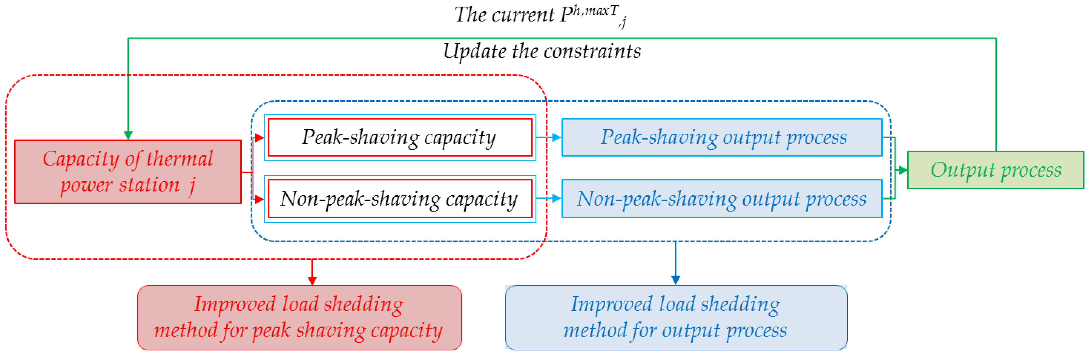
Based on the ILSM [3] and the idea of a nested structure, the typical daily output process of a single thermal power station can be divided into two parts: the peak shaving output process, and the non-peak shaving output process. It can be regarded as the output process that is worked out with peak-shaving capacity and non-peak-shaving capacity of the thermal power station by using the ILSM. This can be viewed as a two-layer nested structure. In the outer layer where the constraint of generated energy is left out, the working capacity of a thermal power station is divided into the peak shaving part and the non-peak shaving part, according to the constraint of peak shaving capacity and the iterative idea of the ILSM. In the inner layer, with the obtained peak shaving and non-peak shaving capacity, the ILSM is used to work out the peak shaving output process and the non-peak shaving output process, respectively. Finally, by adding the two processes together, the typical daily output process of the thermal power station is produced. In the case of multiple TPS for calculation, the method of the available capacity’s daily utilized hours is used to determine the calculation order of the TPS. The calculation principle is illustrated in Figure 1.
3.2. Basic Constraints
In the balance calculation of the electric power and energy of a thermal power station, there are some constraints that need to be satisfied.
The upper and lower limits of output:
where and are the lower limit and the upper limit of output of thermal power station j in MW, respectively; is the output of thermal power station j in the hth period in MW; and h is the index for a certain time period, ranging from 1 to 24.
The constraint of peak shaving capacity:
where and are the minimum and maximum typical daily output of thermal power station j in MW, respectively; is the peak shaving capacity of thermal power station j in MW; and εj is the peak shaving capacity factor of thermal power station j.
The ramping constraint:
where is the ramping ability of thermal power station j in the contiguous period in MW.
The constraint of generated energy:
where is the typical daily average output of thermal power station j in MW.
The constraint of electric power:
And all of the parameters are non-negative.
3.3. Calculation Order
According to the method of available capacity’s daily utilized hours [11,12], the order in which each thermal power station should be calculated is determined by its available capacity’s daily utilized hours. The fewer the available capacity’s daily utilized hours, the earlier the thermal power station is calculated.
3.4. Calculation of the Power System’s Remaining Load
The load that thermal power station j undertakes is the power system’s remaining load after the calculation of all hydropower stations and TPS 1 to j−1, which can be expressed as follows:
where is the power system’s remaining load in the hth period in MW; Nh is the power system’s load in the hth period in MW; is the output of hydropower station i in the hth period in MW; and is the output of thermal power station j in the hth period in MW.
3.5. Calculation Steps of the Nested-Structured Load Shedding Method
This paper does away with the approach that groups TPS together to jointly undertake the power system’s remaining load, which is the case when using the traditional load shedding method. As an alternative, the calculation of TPS is conducted one by one, in the same way that hydropower stations are treated. However, because of the constraint of peak shaving capacity, TPS are different from hydropower stations, whose whole working capacity can be used for shaving peak load. So the remaining load of the power system is divided into two parts: the constant base load and the varying load (such as peak load or waist load). Firstly, the peak shaving capacity of a thermal power station is taken into the constraint of electric power, its typical energy generated daily is taken into the constraint of generated energy, and the ILSM is employed to shed the power system’s varying load. Then, the power constraint is changed to involve the remaining working capacity of the thermal power station, while the energy constraint is changed to involve its remaining typical daily generated energy left by the preceding calculation. Next, the load shedding method is applied to shed the system’s base load. By adding the two resulted output processes together, the typical daily output process of the thermal power station can be obtained. The detailed calculation procedure is described as follows.
Step 1: Calculate the generated power corresponding to the power system’s remaining load, according to the following formula:
where E is the generated power corresponding to the power system’s remaining load in MW∙h; and t is the duration of the hth period.
Divide the power system’s remaining load into the varying load and the constant base load:
where and are the varying load and the constant base load of the power system’s remaining load in the hth period in MW, respectively; and is the minimum load of the power system in MW.
Step 2: Calculate the peak shaving capacity of thermal power station j according to Formula (23). Initially, the maximum working capacity of the thermal power station is assumed to be its maximum output.
Step 3: With the peak shaving capacity and the typical daily generated energy of thermal power station j being constrained, use the ILSM [3] to shed the power system’s varying load to get the peak shaving output process and typical daily generated energy of thermal power station j.
where is the peak shaving generated energy of thermal power station j on a typical day in MW∙h; and is the peak shaving output of thermal power station j in the hth period in MW.
Step 4: Calculate the remaining generated energy and working capacity required of thermal power station j:
where is the remaining generated energy required of thermal power station j on the typical day in MW∙h; and is the remaining working capacity required of thermal power station j in MW.
Step 5: If:
where is the peak shaving capacity required of thermal power station j in MW, the remaining working capacity of thermal power station j cannot meet its electricity demand. So, it is necessary to reduce its peak shaving capacity in order to generate less peak shaving energy until the condition expressed by Formula (37) is met. Use the load shedding method to iteratively calculate the peak shaving capacity of thermal power station j, and determine the iterative step size (δ) by the following formula:
Return to Step 3 for recalculation until the condition expressed by Formula (37) is satisfied.
Step 6: If
Then, the remaining output of thermal power station j left for the constant base load is:
where is the non-peak shaving output of thermal power station j in the hth period in MW.
Step 7: Add up the two separated output processes of thermal power station j to produce its typical daily output process:
If
where and are the maximum and minimum of in MW, the peak shaving capacity of thermal power station j is too large. Use the load shedding method to iteratively calculate the peak shaving capacity of thermal power station j, and determine the iterative step size (δ) by the following formula:
Then, return to Step 3 for recalculation until Formula (43) is satisfied.
Step 8: If
Then, calculate the power system’s remaining load, and the procedure goes on to the next thermal power station. The entire calculation process is illustrated by Figure 2.
4. Case Study and Result Analysis
4.1. Basic Information
In this paper, a region in southwest China is taken as the research area for case study, where the flood season of a dry year is from June to October, and the rest of the year pertains to the non-flood season. Table 1 shows the maximum monthly load and monthly average load of a power system in this region, while Table 2 shows the hourly load rate on a typical day during both flood season and non-flood season. Plus, the expected monthly average output of a hydropower station group (HPSG), the minimum monthly output of six TPS and the installed capacity of each power station are shown in Table 3, Table 4 and Table 5, respectively.
The method introduced in this paper is used to calculate the monthly adjustment coefficients as well as the power and energy balance within a year, a month, and over a typical day. The power system’s RC is set at 10% of the annual maximum load, while the peak shaving capacity of TPS is equal to 25% (εj = 25%). All of the monthly adjustment coefficients of both the hydropower and TPS are less than 1.2, and the annual idle capacity (IC) is used for the maintenance of power stations’ generator units.
With the given data, we use the NSLSM and the ILSM respectively, to calculate the balance of electric power and energy, and then compare and analyze the results.
4.2. Result Analysis of the Electric Power and Energy Balance
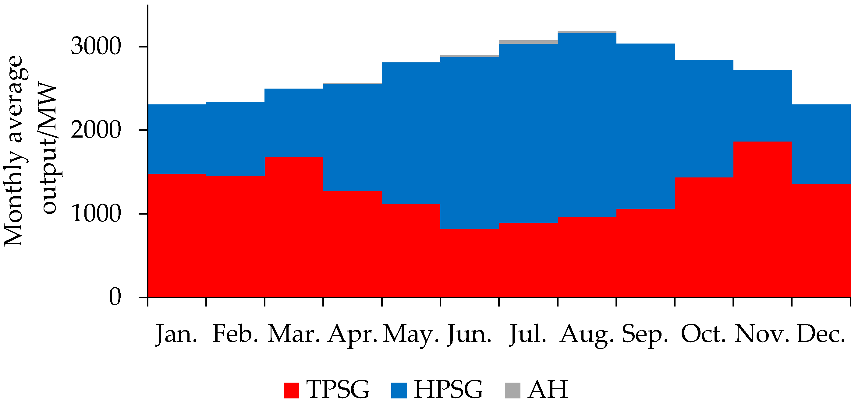
Figure 3 and Figure 4 show the results of the power system’s electric power balance in the dry year, which are obtained by using the NSLSM and the ILSM, respectively. Figure 5 and Figure 6 show the results of the power system’s electric energy balance in the dry year, which are obtained by using the two methods, respectively.
From Figure 3 to Figure 6, it can be seen that the ILSM can only take all of the TPS as one single power station to participate in the calculation, thus obtaining the result of electric power and energy balance of the thermal power station group (TPSG). Whereas for the NSLSM, each thermal power station independently participates in the calculation, and then gets its own result. Since the NSLSM is based on the principle of the ILSM, the results for the electric power and energy balance of the whole TPSG calculated by the two methods show roughly the same trend. The difference is that when using the NSLSM, the monthly average output of the TPSG from June to August is greater, and its maximum typical daily output is smaller, compared with using the ILSM. In Figure 5, the abandoned hydropower of the power system from June to August is greater than that shown in Figure 6. The reason is that when using the NSLSM, each thermal power station needs to be separately calculated for energy balance and power balance. Limited by the constraints of peak shaving capacity and monthly adjustment coefficients, TPS 3 and TPS 4 have to be operated at full capacity, and cannot carry out the task of shaving peak load. Therefore, the monthly average output of the TPSG is quite large. To adjust the load/energy fluctuation of the power system, the TPSG presents a weak peak-shaving capacity and a small maximum output. In contrast, when using the ILSM, the TPSG participates in the calculation as a whole, with a stronger ability to adjust the power system’s load/energy fluctuation. As a result, the monthly average output of the TPSG is smaller and, with more capacity harnessed for peak load regulation, its maximum output is relatively larger.
4.3. Analysis of Peak-Shaving Capacity
The peak shaving capacity of each power station between June and August in the dry year is shown in Table 6.
It is demonstrated in Table 6 that from June to August, the TPS not only solve the problems of load fluctuation and energy balance of the power system through energy modulation, but also take on the task of shaving peak load to achieve power balance. In June, only TPS 1 participates in shaving the peak load of the power system. This is because for TPS 1, the number of its available capacity’s daily-utilized hours is the smallest out of all of the TPS, making it the first one to be calculated, after which there is no peak load or waist load left in the power system. In July, while TPS 1, TPS 2, and TPS 5 participate in shaving the peak load of the power system, TPS 3 and TPS 4 are unable to do so because of the constraints of their peak shaving capacity, and the fact that they need to adjust their generated energy in order to achieve the power system’s energy balance. When calculating TPS 6, there is no peak load or waist load left for it to shave or regulate. In August, while TPS 1, TPS 2, TPS 5, and TPS 6 participate in shaving peak load, TPS 3 and TPS 4 cannot do so due to the same reason mentioned above. From the result of using the ILSM, it can only be obtained that the TPSG does shave peak load from June to August, without figuring out the exact value of a specific station’s peak shaving capacity.
4.4. Analysis of Monthly Adjustment Coefficients
The monthly adjustment coefficient of each power station in the dry year is shown in Table 7.
In the dry year, the monthly adjustment coefficients of the power system are 1.090 in non-flood season, and 1.114 in flood season. It can be seen from Table 7 that the adjustment coefficients of all of the power stations meet the basic requirements of the power system’s routine operation. While the TPS regulate their power output to meet the demand of the power system’s monthly energy fluctuations throughout the year, the hydropower stations attain the same goal from June to August by abandoning water to change their power output.
5. Conclusions
This paper analyzed the monthly load fluctuations of power systems in order to regulate, the monthly and daily generated energy of TPS in a way that meets the load demand of the power system. A new method (NSLSM) is proposed to calculate the balance of electric power and energy of TPS, based on the theory of the traditional load shedding method. Iterative computation is conducted on the peak shaving capacity of a single thermal power station, so as to yield its energy benefit and peak shaving benefit, while also satisfying the power system’s load demand.
According to the calculation results, by using the NSLSM, the monthly average output of the TPSG rises, and its peak shaving capacity reduces, which leads to the abandoned hydropower energy of the system increasing. However, this method can also produce the monthly average output and typical daily average output of each thermal power station, thus reflecting the stability of thermal power output within a month. Additionally, the peak shaving capacity of each thermal power station can be obtained directly, and with these more accurate results, we can conduct further study concerning problems such as the coal consumption and economic operation of each thermal power station. Compared with traditional methods, this new method of calculating power and energy balance can produce the typical daily output process of every thermal power station, without blurring or averaging out the typical daily output processes and peak shaving capacity of different TPS.
Acknowledgments
This work was supported by the "13th Five-Year" National Key Research and Development Program of China under Grand Nos. 2016YFC0402208, 2016YFC0402308, 2016YFC0402309 and the Natural Science Foundation of China under Grand Nos. 51279062, 51679088.
Author Contributions
Minghao Liu conceived the main idea and wrote the manuscript with guidance from Liping Wang. Boquan Wang, Jiajie Wu and Chuangang Li reviewed the work and gave helpful improvement suggestions.
Conflicts of Interest
The authors declare no conflict of interest.
References
- Cheng, C.T.; Shen, J.J.; Wu, X.Y.; Chau, K.W. Operation challenges for fast-growing China’s hydropower systems and respondence to energy saving and emission reduction. Renew. Sustain. Energy Rev. 2012, 16, 2386–2393. [Google Scholar] [CrossRef]
- Xu, B.; Zhong, P.A.; Wan, X.Y.; Zhang, W.G.; Chen, X. Dynamic Feasible Region Genetic Algorithm for Optimal Operation of a Multi-Reservoir System. Energies 2012, 5, 2894–2910. [Google Scholar] [CrossRef]
- Kuo, M.T.; Lu, S.D. Experimental Research and Control Strategy of Pumped Storage Units Dispatching in the Taiwan Power System Considering Transmission Line Limits. Energies 2013, 6, 3224–3244. [Google Scholar] [CrossRef]
- Cheng, C.T.; Wang, S.; Chau, K.W.; Wu, X.Y. Parallel discrete differential dynamic programming for multireservoir operation. Environ. Model. Softw. 2014, 57, 152–164. [Google Scholar] [CrossRef]
- Guo, S.L.; Chen, J.H.; Li, Y.; Liu, P.; Li, T.Y. Joint operation of the multi-reservoir system of the Three Gorges and the Qingjiang cascade reservoirs. Energies 2011, 4, 1036–1050. [Google Scholar] [CrossRef]
- Shao, L.; Wang, L.P.; Huang, H.T.; Yang, Z.; Yu, S. Optimization of the reservoir operation chart of hydropower station and its application–Based on hybrid genetic algorithm and simulated annealing. Power Syst. Prod. Control 2010, 38, 40–43. [Google Scholar]
- Li, G. Short Term Energy Saving Power Generation Operation of Hydro Thermal Power System; Dalian University of Technology: Dalian, China, 2007. [Google Scholar]
- Cai, J.Z.; Cai, H.X.; Hong, G.P. The research and application on electric power and energy balance. Yunnan Electr. Power Technol. 1994, 3, 8–11. [Google Scholar]
- Wu, D.P.; Wan, Y.H. Residual load successive shift method of electric power balance. J. Hydroelectr. Power Gener. 1994, 3, 31–36. [Google Scholar]
- Pang, F. The new method about electric power and energy balance. J. Hydroelectr. Eng. 2001, 20, 117–123. [Google Scholar]
- Ma, G.W.; Wang, L. Study on working position of hydropower station in electric power system. J. Hydroelectr. Eng. 1992, 1, 39–46. [Google Scholar]
- Liao, S.L.; Cheng, C.T.; Cai, H.X.; Cai, J.Z.; Wu, D.P. Improved algorithm of adjusting discharge peak by thermal power plants. Autom. Electr. Power Syst. 2006, 30, 89–93. [Google Scholar]
- Wang, J.Y.; Shen, J.J.; Cheng, C.T.; Lu, J.Y.; Li, G. A load shedding method for thermal power plants with peak regulation based on load reconstruction strategy. Trans. China Electrotech. Soc. 2014, 34, 2684–2691. [Google Scholar]
- Zhang, R.; Zhou, J.; Ouyang, S.; Wang, X.; Zhang, H. Optimal operation of multi-reservoir system by multi-elite guide particle swarm optimization. Int. J. Electr. Power Energy Syst. 2013, 48, 58–68. [Google Scholar] [CrossRef]
- Zhang, W.; Lian, J.; Chang, C.Y.; Kalsi, K. Aggregated Modeling and Control of Air Conditioning Loads for Demand Response. IEEE Trans. Power Syst. 2013, 28, 4655–4664. [Google Scholar] [CrossRef]
- Xu, J.; Gu, Y.; Chen, D.; Li, Q. Data mining based plant-level load dispatching strategy for the coal-fired power plant coal-saving: A case study. Appl. Therm. Eng. 2017, 119, 553–559. [Google Scholar] [CrossRef]
- Selakov, A.; Cvijetinović, D.; Milović, L.; Mellon, S.; Bekut, D. Hybrid PSO-SVM method for short-term load forecasting during periods with significant temperature variations in city of Burbank. Appl. Soft Comput. 2014, 16, 80–88. [Google Scholar] [CrossRef]
- Wang, N.; Zhang, Y.; Zhang, T.; Yang, Y. Data Mining-Based Operation Optimization of Large Coal-Fired Power Plants. Aasri Procedia 2012, 3, 607–612. [Google Scholar] [CrossRef]
- Blanco, J.M.; Vazquez, L.; Peña, F.; Diaz, D. New investigation on diagnosing steam production systems from multivariate time series applied to thermal power plants. Appl. Energy 2013, 101, 589–599. [Google Scholar] [CrossRef]
- Li, L.; Tan, Z.; Wang, J.; Xu, J.; Cai, C.; Hou, Y. Energy conservation and emission reduction policies for the electric power industry in China. Energy Policy 2011, 39, 3669–3679. [Google Scholar] [CrossRef]
- Shan, B.G.; Xu, M.J.; Zhu, F.G.; Zhang, C.L. China’s Energy Demand Scenario Analysis in 2030. Energy Procedia 2012, 14, 1292–1298. [Google Scholar] [CrossRef]
- Yu, X.M.; Xiong, X.Y.; Wu, Y.W. Discussion on optimal model for peaking units’ expansion planning and its application. Electr. Power 2003, 36, 48–51. [Google Scholar]
- Billinton, R.; Ge, J. A comparison of four-state generating unit reliability models for peaking units. IEEE Trans. Power Syst. 2004, 19, 763–768. [Google Scholar] [CrossRef]
- Park, H.G.; Lyu, J.K.; Kang, Y.; Park, J.K. Unit Commitment Considering Interruptible Load for Power System Operation with Wind Power. Energies 2014, 7, 4281–4299. [Google Scholar] [CrossRef]
Figure 1.
Schematic diagram of the nested-structured load shedding method (NSLSM).

Figure 2.
Calculation flow chart of the NSLSM.
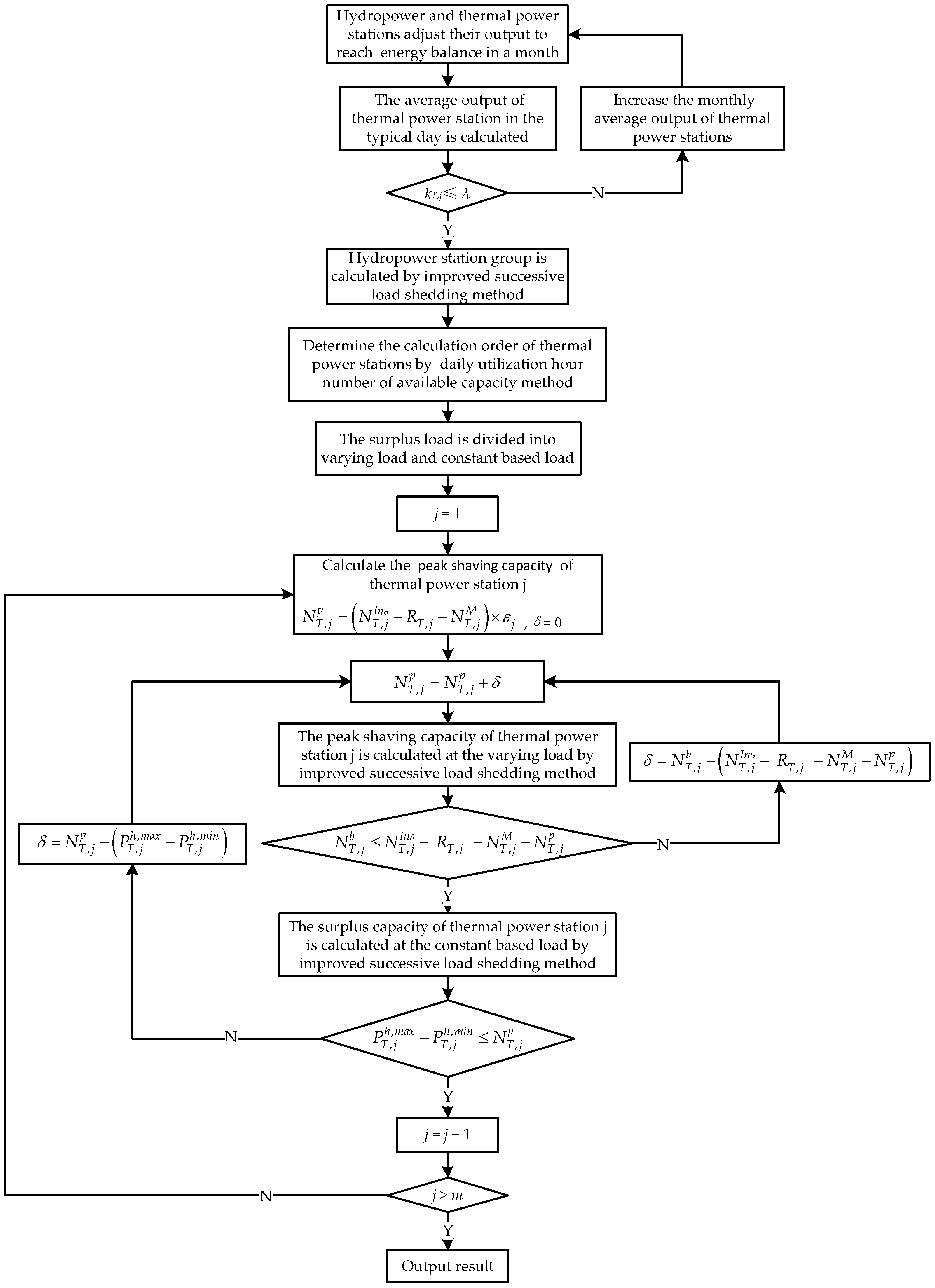
Figure 3.
Power balance diagram of the power system in a dry year using the NSLSM; HPSG: hydropower station group; IC: idle capacity; MC: maintenance capacity; RC: reserve capacity.
Figure 3.
Power balance diagram of the power system in a dry year using the NSLSM; HPSG: hydropower station group; IC: idle capacity; MC: maintenance capacity; RC: reserve capacity.
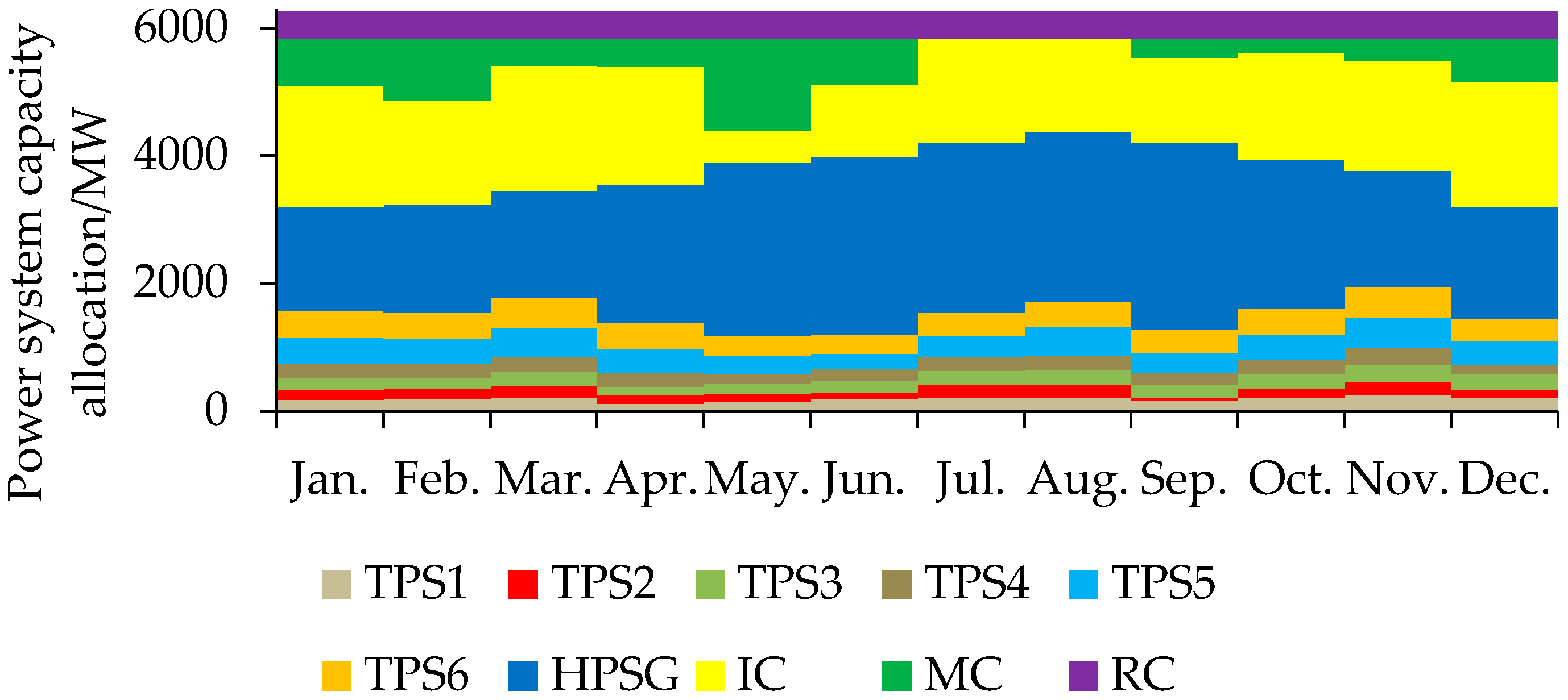
Figure 4.
Power balance diagram of the power system in dry year using the improved load shedding method (ILSM). TPSG: thermal power station group
Figure 4.
Power balance diagram of the power system in dry year using the improved load shedding method (ILSM). TPSG: thermal power station group
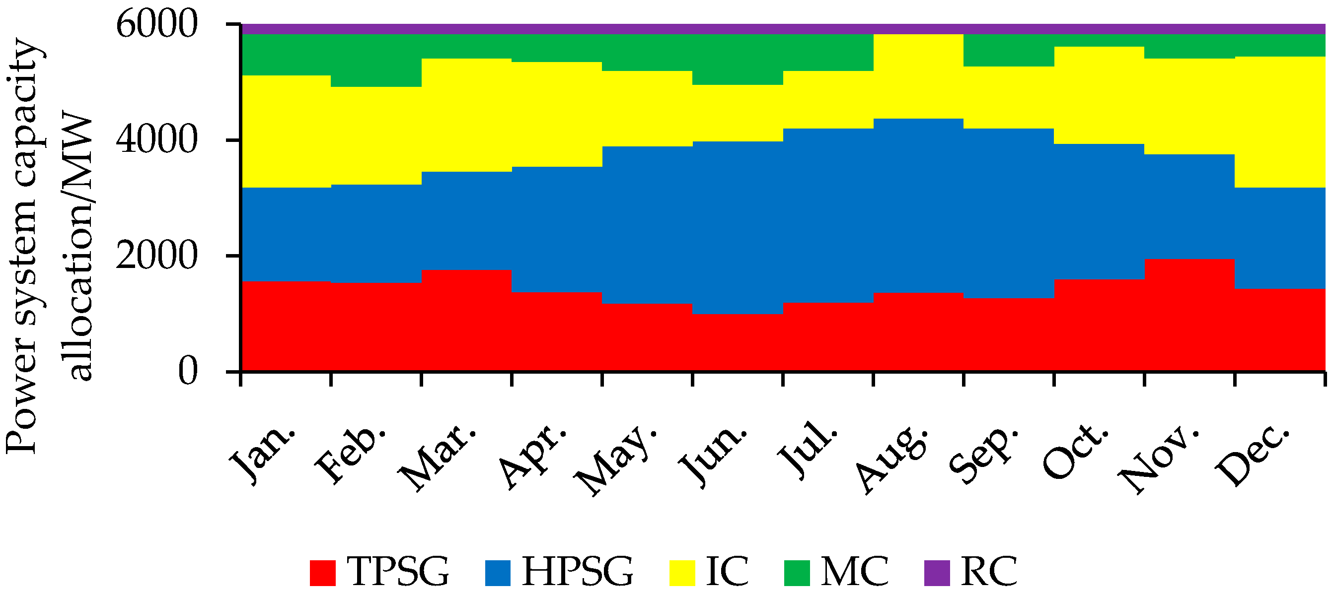
Figure 5.
Energy balance diagram of the power system in dry year (using the NSLSM). AH: abandoned hydropower energy
Figure 5.
Energy balance diagram of the power system in dry year (using the NSLSM). AH: abandoned hydropower energy
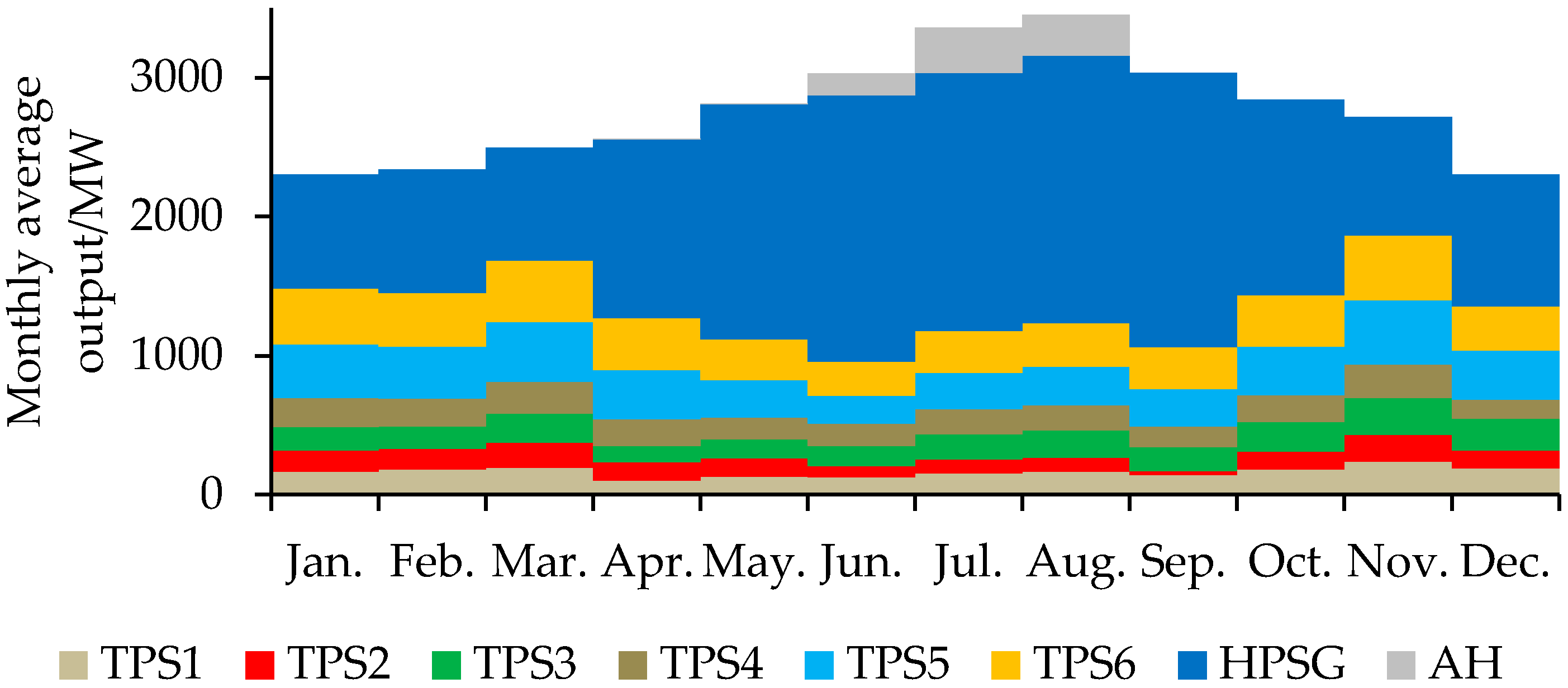
Figure 6.
Energy balance diagram of the power system in dry year (using the ILSM).

Table 1.
Maximum monthly load and monthly average load of the power system (Unit: MW).
| Month | Maximum Load | Average Load | Month | Maximum Load | Average Load |
|---|---|---|---|---|---|
| January | 3190 | 2305 | Jul. | 4200 | 3035 |
| February | 3235 | 2338 | Aug. | 4375 | 3161 |
| March | 3455 | 2496 | Sep. | 4200 | 3035 |
| April | 3540 | 2558 | Oct. | 3935 | 2843 |
| May | 3890 | 2811 | Nov. | 3760 | 2717 |
| June | 3980 | 2876 | Dec. | 3190 | 2305 |
Table 2.
Hourly load rate on the typical day in flood and non-flood seasons.
| Time | Flood Season | Non-Flood Season | Time | Flood Season | Non-Flood Season |
|---|---|---|---|---|---|
| 1 | 0.68 | 0.65 | 13 | 0.83 | 0.8 |
| 2 | 0.63 | 0.60 | 14 | 0.80 | 0.86 |
| 3 | 0.58 | 0.56 | 15 | 0.91 | 0.85 |
| 4 | 0.57 | 0.55 | 16 | 0.97 | 0.98 |
| 5 | 0.56 | 0.53 | 17 | 0.96 | 1.00 |
| 6 | 0.54 | 0.52 | 18 | 0.93 | 0.97 |
| 7 | 0.56 | 0.55 | 19 | 0.94 | 0.94 |
| 8 | 0.61 | 0.60 | 20 | 1.00 | 0.9 |
| 9 | 0.75 | 0.74 | 21 | 0.99 | 0.93 |
| 10 | 0.90 | 0.88 | 22 | 0.94 | 0.99 |
| 11 | 0.96 | 0.93 | 23 | 0.83 | 0.95 |
| 12 | 0.96 | 0.95 | 24 | 0.74 | 0.84 |
Table 3.
Monthly average output of the hydropower stations (HPS) (Unit: MW/h).
| Month | HPS 1 | HPS 2 | HPS 3 | HPS 4 | HPS 5 | HPS 6 | HPS 7 | HPS 8 |
|---|---|---|---|---|---|---|---|---|
| January | 127.0 | 60.1 | 162.7 | 236.6 | 48.6 | 85.3 | 36.3 | 67.1 |
| February | 172.0 | 68.1 | 157.7 | 236.5 | 49.6 | 93.0 | 39.7 | 68.1 |
| March | 156.0 | 76.5 | 134.8 | 237.2 | 41.9 | 101.1 | 43.1 | 22.5 |
| April | 101.0 | 88.7 | 112.0 | 238.8 | 61.9 | 381.5 | 273.3 | 30.6 |
| May | 68.0 | 207.9 | 247.3 | 239.8 | 71.4 | 534.9 | 228.4 | 97.3 |
| June | 136.6 | 287.0 | 379.8 | 240.7 | 139.9 | 572.8 | 189.4 | 127.4 |
| July | 145.9 | 273.7 | 456.0 | 254.7 | 135.0 | 600.0 | 238.0 | 76.0 |
| August | 175.5 | 323.3 | 389.4 | 287.6 | 140.2 | 572.8 | 267.5 | 61.7 |
| September | 136.8 | 218.4 | 400.9 | 257.7 | 112.9 | 525.0 | 243.7 | 76.4 |
| October | 125.7 | 200.4 | 271.5 | 267.3 | 83.6 | 268.7 | 131.2 | 56.2 |
| November | 70.0 | 116.5 | 154.6 | 251.4 | 53.4 | 115.7 | 27.8 | 61.8 |
| December | 94.0 | 196.0 | 163.7 | 239.4 | 47.9 | 98.5 | 42.1 | 67.0 |
Table 4.
Minimum monthly output of the thermal power stations (TPS) (Unit: MW/h).
| Month | TPS 1 | TPS 2 | TPS 3 | TPS 4 | TPS 5 | TPS 6 |
|---|---|---|---|---|---|---|
| January | 30.0 | 30.0 | 40.0 | 100.0 | 200.0 | 200.0 |
| February | 70.0 | 30.0 | 50.0 | 100.0 | 200.0 | 200.0 |
| March | 40.0 | 30.0 | 60.0 | 100.0 | 200.0 | 200.0 |
| April | 56.7 | 30.0 | 70.0 | 100.0 | 200.0 | 200.0 |
| May | 61.7 | 30.0 | 80.0 | 100.0 | 200.0 | 200.0 |
| June | 66.7 | 30.0 | 90.0 | 100.0 | 200.0 | 200.0 |
| July | 71.7 | 30.0 | 100.0 | 100.0 | 200.0 | 200.0 |
| August | 76.7 | 30.0 | 110.0 | 100.0 | 200.0 | 200.0 |
| September | 81.7 | 30.0 | 120.0 | 100.0 | 200.0 | 200.0 |
| October | 86.7 | 30.0 | 130.0 | 100.0 | 200.0 | 200.0 |
| November | 91.7 | 30.0 | 140.0 | 100.0 | 200.0 | 200.0 |
| December | 96.7 | 30.0 | 150.0 | 100.0 | 200.0 | 200.0 |
Table 5.
Installed capacity of each power station.
| Power Station | HPS 1 | HPS 2 | HPS 3 | HPS 4 | HPS 5 | HPS 6 | HPS 7 |
| Installed Capacity (MW) | 300 | 370 | 630 | 540 | 150 | 600 | 300 |
| Power Station | HPS 8 | TPS 1 | TPS 2 | TPS 3 | TPS 4 | TPS 5 | TPS 6 |
| Installed Capacity (MW) | 180 | 400 | 400 | 400 | 400 | 800 | 800 |
Table 6.
Peak shaving capacity of each power station from June to August (Unit: MW/h).
| Method | NSLSM | ILSM | ||||
|---|---|---|---|---|---|---|
| Power Station | TPS 1 | TPS 2 | TPS 3 | TPS 4 | TPS 5 | TPSG |
| June | 43.58 | 0 | 0 | 0 | 0 | 43.58 |
| July | 27.81 | 89.16 | 0 | 0 | 22.06 | 139.03 |
| August | 7.98 | 89.19 | 0 | 0 | 159.41 | 260.97 |
Table 7.
Monthly adjustment coefficient of each power station in the dry year.
| Month | HPS 1 | HPS 2 | HPS 3 | HPS 4 | HPS 5 | HPS 6 | HPS 7 |
| January | 1.150 | 1.150 | 1.150 | 1.150 | 1.150 | 1.150 | 1.150 |
| February | 1.140 | 1.140 | 1.140 | 1.140 | 1.140 | 1.140 | 1.140 |
| March | 1.174 | 1.174 | 1.174 | 1.174 | 1.174 | 1.174 | 1.174 |
| April | 1.099 | 1.099 | 1.099 | 1.099 | 1.099 | 1.099 | 1.099 |
| May | 1.112 | 1.112 | 1.112 | 1.112 | 1.112 | 1.112 | 1.112 |
| June | 1.085 | 1.062 | 1.081 | 1.086 | 1.062 | 1.062 | 1.073 |
| July | 1.087 | 1.067 | 1.061 | 1.091 | 1.040 | 1.039 | 1.042 |
| August | 1.083 | 1.045 | 1.076 | 1.088 | 1.041 | 1.040 | 1.042 |
| September | 1.068 | 1.068 | 1.068 | 1.068 | 1.068 | 1.068 | 1.068 |
| October | 1.116 | 1.116 | 1.116 | 1.116 | 1.116 | 1.116 | 1.116 |
| November | 1.188 | 1.188 | 1.188 | 1.188 | 1.188 | 1.188 | 1.188 |
| December | 1.133 | 1.133 | 1.133 | 1.133 | 1.133 | 1.133 | 1.133 |
| Month | HPS 8 | TPS 1 | TPS 2 | TPS 3 | TPS 4 | TPS 5 | TPS 6 |
| January | 1.150 | 1.057 | 1.057 | 1.057 | 1.057 | 1.057 | 1.057 |
| February | 1.140 | 1.059 | 1.059 | 1.059 | 1.059 | 1.059 | 1.059 |
| March | 1.174 | 1.050 | 1.050 | 1.050 | 1.050 | 1.050 | 1.050 |
| April | 1.099 | 1.080 | 1.080 | 1.080 | 1.080 | 1.080 | 1.080 |
| May | 1.112 | 1.056 | 1.056 | 1.056 | 1.056 | 1.056 | 1.056 |
| June | 1.064 | 1.199 | 1.199 | 1.199 | 1.199 | 1.199 | 1.199 |
| July | 1.093 | 1.199 | 1.199 | 1.199 | 1.199 | 1.199 | 1.199 |
| August | 1.094 | 1.199 | 1.199 | 1.199 | 1.199 | 1.199 | 1.199 |
| September | 1.068 | 1.197 | 1.197 | 1.197 | 1.197 | 1.197 | 1.197 |
| October | 1.116 | 1.111 | 1.111 | 1.111 | 1.111 | 1.111 | 1.111 |
| November | 1.188 | 1.045 | 1.045 | 1.045 | 1.045 | 1.045 | 1.045 |
| December | 1.133 | 1.060 | 1.060 | 1.060 | 1.060 | 1.060 | 1.060 |
© 2017 by the authors. Licensee MDPI, Basel, Switzerland. This article is an open access article distributed under the terms and conditions of the Creative Commons Attribution (CC BY) license (http://creativecommons.org/licenses/by/4.0/).
Share and Cite
MDPI and ACS Style
Wang, L.; Liu, M.; Wang, B.; Wu, J.; Li, C. Study on Nested-Structured Load Shedding Method of Thermal Power Stations Based on Output Fluctuations. Energies 2017, 10, 1472. https://doi.org/10.3390/en10101472
AMA Style
Wang L, Liu M, Wang B, Wu J, Li C. Study on Nested-Structured Load Shedding Method of Thermal Power Stations Based on Output Fluctuations. Energies. 2017; 10(10):1472. https://doi.org/10.3390/en10101472
Chicago/Turabian StyleWang, Liping, Minghao Liu, Boquan Wang, Jiajie Wu, and Chuangang Li. 2017. "Study on Nested-Structured Load Shedding Method of Thermal Power Stations Based on Output Fluctuations" Energies 10, no. 10: 1472. https://doi.org/10.3390/en10101472
Note that from the first issue of 2016, this journal uses article numbers instead of page numbers. See further details here.