Global Gust Climate Evaluation and Its Influence on Wind Turbines

Environmental Meteorology, University of Freiburg, 79085 Freiburg, Germany
*
Author to whom correspondence should be addressed.
Energies 2017, 10(10), 1474; https://doi.org/10.3390/en10101474
Submission received: 8 August 2017
/
Revised: 18 September 2017
/
Accepted: 19 September 2017
/
Published: 23 September 2017
(This article belongs to the Special Issue Risk-Based Methods Applied to Power and Energy Systems)
Abstract
:Strong gusts negatively affect wind turbines in many ways. They (1) harm their structural safety; (2) reduce their wind energy output; and (3) lead to a shorter wind turbine rotor blade fatigue life. Therefore, the goal of this study was to provide a global assessment of the gust climate, considering its influence on wind turbines. The gust characteristics analyzed were: (1) the gust speed return values for 30, 50 and 100 years; (2) the share of gust speed exceedances of cut-out speed; and (3) the gust factor. In order to consider the seasonal variation of gust speed, gust characteristics were evaluated on a monthly basis. The global monthly wind power density was simulated and geographical restrictions were applied to highlight gust characteristics in areas that are generally suitable for wind turbine installation. Gust characteristics were computed based on ERA-interim data on a 1° × 1° spatial resolution grid. After comprehensive goodness-of-fit evaluation of 12 theoretical distributions, Wakeby distribution was used to compute gust speed return values. Finally, the gust characteristics were integrated into the newly developed wind turbine gust index. It was found that the Northeastern United States and Southeast Canada, Newfoundland, the southern tip of South America, and Northwestern Europe are most negatively affected by the impacts of gusts. In regions where trade winds dominate, such as eastern Brazil, the Sahara, southern parts of Somalia, and southeastern parts of the Arabian Peninsula, the gust climate is well suitable for wind turbine installation.
1. Introduction
Constant electricity supply is essential for both production and consumption of goods and services [1]. Extreme weather conditions can have serious negative impacts on the electricity supply. Windstorms and tropical storms are amongst the most harmful disturbances for the electricity grid [2]. Minor storm-related power outages are mainly caused by damage from trees falling on local electricity distribution lines and poles, while major outages are often the result of damage to electricity transmission lines [3,4]. In the USA alone, it is estimated that storm-related outages cost between $20 billion and $55 billion annually [3].
The utilization of wind energy poses new challenges to storm risk management in the energy industry. Wind turbines are used to convert the kinetic energy of airflow first into mechanical and then into useful electric energy [5]. In order to maximize power output, wind turbines are generally built in areas where average wind speed (x) is high. However, during storm events, x can reach a destructive level. The short-time (~3 s) fluctuations of x, which are called gusts [6], are a critical issue to the infrastructure and environment [7].
There are several ways gust characteristics (GC) influence wind turbines. First and foremost, extreme gust speed (GS) poses a great risk to the structural safety of wind turbines [8]. The survival speed indicates until which GS a wind turbine stays unharmed. Typical survival speed values are in the range between GS = 50 m s−1 and GS = 70 m s−1 [9]. The wind turbine design is typically developed based on the 50-year return value of GS to consider the most severe storm events [10].
In order to prevent damage, wind turbines are shut down at cut-out speed [11], although x and wind power density (WPD) are high. A typical cut-out speed of many wind turbines is 25.0 m∙s−1. Frequent shut-downs can lead to energy yield losses.
Strong vertical wind shear and gustiness negatively influence the technical integrity of wind turbines. For instance, gustiness reduces the rotor blade fatigue life [12]. Gustiness of the airflow is typically expressed by the gust factor (GF). GF is defined as the ratio between GS and x [13].
The following example emphasizes the importance of GC for the wind energy sector: In 2005, winter storm Gudrun passed over Ireland, Great Britain, Denmark, Norway, and Sweden. On the coast of Denmark, gust speed reached values up to 46 m s−1 in 10 m above ground level (a.g.l.). At that time, 5400 wind turbines operated in Denmark. There was great danger that the survival speed of the wind turbines could be surpassed by the storm-related gusts and a great number of the wind turbines would be damaged by the storm. In order to prevent damage, most wind turbines were shut down after GS exceeded cut-out speed. This led to a sharp decrease in the produced amount of wind energy locally, to less than 5%. The abruptly missing wind energy had to be substituted by energy imports from neighboring countries [14].
Despite its importance, little research involving GC has been carried out [8]. Often theoretical distributions are used to describe the long-term gust climate. In several studies the two-parameter Gumbel distribution (Gu) was applied to capture extreme x characteristics [15,16,17,18]. The three-parameter Generalized Extreme Value distribution (GEV) and Gu were used for extreme x value estimation in China [8]. Morgan et al. Reference [10] evaluated the capability of numerous theoretical distributions to capture the extreme tails of x values in North American offshore areas and found that the two-parameter Lognormal distribution (L) is suitable. The two-parameter Weibull distribution (Wei) was applied by [19] and the three-parameter inverse Burr distribution by [20] to evaluate extreme x values.
The abovementioned studies mainly focused on GC on a regional level. However, as electricity consumption is covered increasingly by wind energy in many countries, it is of great interest and importance to evaluate where, when, and how frequently GS values dangerous for regular, continuous wind turbine operation occur. Thus, a detailed description of the global gust climate is an essential precondition for a comprehensive assessment of gust-related hazards to wind turbine operation, especially in the light of large-scale storm events. The diversity of the conceptual frameworks, samples and results reported from previous studies does not allow for such a general and global description of GC.
Thus, the goal of this investigation is to systematically analyze the (1) long-term return values of GS, (2) occurrences of GS exceeding the wind turbine cut-out speed, and (3) GF on a global scale. For a global overview of the influence of gusts on wind turbines, these GC are integrated into the newly developed wind turbine gust index (WTGI).
2. Material and Methods
2.1. Overview
In order to evaluate GC and to determine WTGI the following steps were carried out: (1) obtaining global grid point related GS and x time series in the period from 1 January 1979 to 31 December 2015; (2) monthly segmentation of GS and x time series; (3) distribution fitting and goodness-of-fit (GoF) evaluation of annual maximum of GS empirical probability density functions (epdf); (4) computation of GS return values for 30 y (GS30yr), 50 y (GS50yr) and 100 y (GS100yr); (5) determination of the monthly cut-out speed exceedances of GS (SOC); (6) calculation of GF using GS as well as x; and (7) integration of GS50yr, SOC and GF into WTGI by normalization.
Distribution fitting of GS was necessary to extrapolate GS values to return levels exceeding the period of available data. The goodness-of-fit of evaluation of various theoretical distributions was carried out in order to determine the most appropriate distribution for calculating the gust speed return values.
2.2. Data
Maximum GS obtainable for a height of 10 m a.g.l. was provided from the ECMWF ERA-Interim reanalysis project [21]. ECMWF ERA-Interim reanalysis gust speed is only available for 10 m a.g.l., which is the standard measuring height for gust speed according to the World Meteorological Organization [22]. The current data base and measurement process of gust speed prevents a globally consistent gust climate evaluation in wind turbine hub height. Thus, an assessment of the global gust climate can best be achieved by using ECMWF ERA-Interim data in 10 m a.g.l. According to the power law [23], gust speed increases with increasing height a.g.l. based on thermally and mechanically induced mixing, wind speed, air temperature conditions, elevation, time of day, season, and the nature of the terrain [12]. Deacon [24] showed that the increase of gust speed with height to be markedly less than the increase of average wind speed. Therefore, gust analysis at 10 m a.g.l. could assess its impact on wind turbines installed at much higher heights.
The reanalysis data cover the entire surface of the earth with grid cells at a spatial resolution of 1° × 1°. The maximum GS values in a three hour period are available for 00 coordinated universal time (UTC), 03 UTC, 06 UTC, 09 UTC, 12 UTC, 15 UTC, 18 UTC and 21 UTC covering the period from 1 January 1979 to 31 December 2015.
Furthermore, the zonal (u) and meridional (v) wind vector components at 00 UTC, 06 UTC, 12 UTC, and 18 UTC in the same period at 10 m a.g.l. were used. The wind vector components were applied to compute average wind speed:
2.3. Distribution Fitting
The GS return values were estimated by the block maxima method using the Matlab version 2017a software (The MathWorks Inc., Natick, MA, USA). This approach is based on the idea that the highest GS values of time-limited blocks (often years) from a parent distribution can be used to estimate GS return values by fitting them to an extreme value distribution [27,28]. The block maxima method was applied by first obtaining the annual maximum GS values for each month. Subsequently, the annual maximum GS time series were transformed into epdfs and empirical cumulative distribution functions (ecdfs). Afterwards, twelve different theoretical distributions were fitted to monthly GS epdfs and ecdfs (Table 1). The number of distribution’s parameters (NP) range from two to five. The parameter estimation methods (PEM) L-moment method (LM), Maximum Likelihood estimation (ML) and Moment method (M) were used to find the parameters of each GS epdf [29].
2.4. Goodness-of-Fit Evaluation
In order to select the most suitable of the theoretical distributions to fit GS epdfs, two GoF metrics were applied. The first GoF metric was the Kolmogorov–Smirnov (KS) statistic [30]. KS is defined as the maximum absolute difference between ecdf and the cumulative distribution function of the theoretical distribution (cdf):
where is the ith ecdf value and is the estimated cdf of the ith ecdf value.
The second GoF metric was the Anderson–Darling (AD) statistic [31]:
where n is the sample size. The lower the KS and AD values, the better the GoF of the theoretical distribution.
2.5. Wakeby Distribution
According to GoF evaluation, Wak is the most appropriate theoretical distribution to characterize GS epdfs. It is defined by one location parameter (ε), two scale parameters (α, γ), and two shape parameters (β, δ). The probability density function (pdf) of Wak is [32]:
2.6. Determination of Gust Characteristics
By applying Wak, GS return values were estimated. The cumulative probabilities related to return periods (T) of 30, 50 or 100 yr were computed by [37]:
Afterwards, it was possible to estimate GS return values by Equation (5) for each grid-cell, month, and T. SOC was determined by counting the grid point-related, monthly cut-out speed (25 m s−1) exceedances of GS in the investigation period. GF was computed by dividing the maximum GS in a six-hour period by x related to the same period. Afterwards, the median of the monthly, six hourly GF values was computed .
2.7. Calculation of Wind Turbine Gust Index
The wind turbine gust index was developed to enable a global comparison of the threat gusts pose to the wind turbine utilization in different regions of the world. For WTGI calculation, the monthly gust characteristics GS50yr, and SOC were normalized according to [38]:
with being the normalized statistic and and are the minimum and maximum original values for the statistic, respectively. Furthermore, all monthly were added up, yielding WTGI. The grid point-related WTGI values were classified into eight classes by quantiles. Thus, class 1 indicates that a location belongs to the 12.5% of geographically accessible area with the least impact of gusts. Accordingly, class 8 indicates that a location belongs to the 12.5% of geographically accessible area with the greatest impact of gusts. The classification was carried out separately for geographically accessible onshore and offshore areas.
2.8. Determination of the Meteorological and Geographical Wind Energy Potential
The meteorological and geographical wind energy potential was evaluated in order to highlight WTGI in areas, which are generally suitable for wind turbine installation.
WPD was used to assess the meteorological wind energy potential, according to:
where is the air density, which was calculated by:
with APR being the atmospheric pressure, TA the air temperature, and R the atmospheric gas constant (287.058 J kg−1 K−1). APR and TA were obtained from ERA-Interim data for the same period as x.
Ice-covered regions, lakes, urban areas, wetlands, evergreen forests [39], conservation areas [40], sloped areas (>10°) [41,42], and permafrost areas [43,44] were excluded using ESRI’s ArcGIS 10.2, since onshore wind turbine installation is not (or only to a limited extent) possible in such regions.
Offshore areas unsuitable for wind turbine installation were defined as areas where the sea depth exceeds 200 m [45].
3. Results and Discussion
3.1. Goodness-of-Fit Evaluation of Gust Speed Distributions
Results of GoF evaluation indicate that Wak-LM is the overall most appropriate theoretical distribution to reproduce GS epdfs. According to KS, Wak-LM fits 42–44% of all evaluated monthly GS epdfs best (Table 2). For two thirds of all GS epdfs, Wak-LM ranked between one and three. No clear GoF differences between onshore and offshore GS epdfs or between GS epdfs related to different months occurred. Thus, it can be assumed that the high fitting accuracy of Wak-LM is not limited to any specific region or month. Therefore, Wak-LM was used to compute monthly GS return values. GEV-LM fits 4–5% of all monthly GS epdfs best and ranked between one and three at ~25% of all grid cells. Other distributions that fit a remarkable number of GS epdfs very well were GL-LM and K-LM. It is striking that PEM of the first eight distributions that ranked most often between one and three was LM. Thus, it can be concluded that LM is the most appropriate PEM for a small sample size. Whereas Wei fitted by LM is at 21–22% of the grid cells among the top three distributions, Wei fitted by M and ML ranked only 1–2% among the three most appropriate distributions.
GoF results obtained for AD are quite similar to KS (Table 3). For more than 60% of all grid cell-related GS epdfs, Wak-LM is among the three top ranked distributions, regardless of month. It provides the highest fitting accuracy for ~50% of all grid cell related epdfs. In contrast to KS, AD is more sensitive to the epdfs tails. Thus, it can be concluded that Wak-LM is suitable for reproducing both the central parts and the upper tails of the evaluated epdfs. The percentage share of GEV-LM ranking between one and three is in all months at least 33%, which is clearly higher than for KS. One reason might be that GEV-LM reproduces the upper tails of the evaluated epdfs very well. It is noticeable that K-LM is the only distribution, beside Wak-LM, that provides the best GoF according to AD for more than 10% of all grid cell related GS epdfs in all months. Other theoretical distributions that provide reasonable fits to GS epdfs are GL-LM, GN-LM and Wei-LM, which rank between one and three for more than 30% at all grid-cell related epdfs in most months. On the other hand, the share of GP-LM, G-ML, L-M, Wei-ML, and Wei-M ranking between one and three is below 3% in all months, indicating that these combinations of theoretical distribution and PEM should not be used for estimating GS return values.
3.2. Gust Characteristics around the World
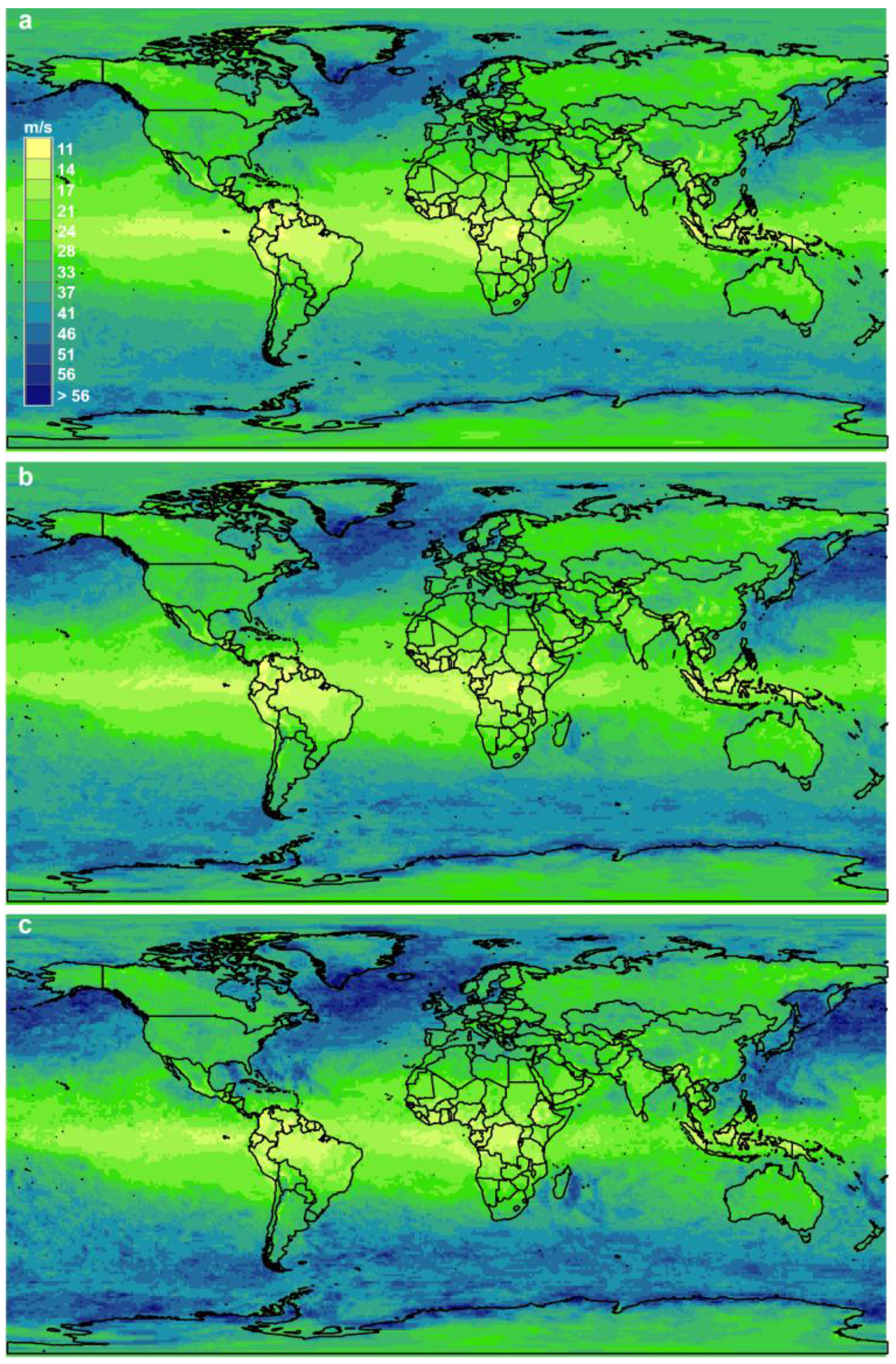
The spatial distribution of GS30yr is characterized by remarkable differences between ocean and land surfaces (Figure 1a). Highest GS30yr values (>40 m s−1) were simulated over the Atlantic Ocean and Pacific Ocean between 40° N to 70° N. At the equator, GS30yr values are clearly lower (<20 m s−1). Near the coasts, GS30yr values are generally lower than on the high seas. Onshore areas where high GS30yr values occur are in the Midwestern United States, Northwestern Europe, and the southern tip of South America. In these regions, GS30yr values exceed 30 m s−1 on large areas. This is a result of the west wind drift in the northern hemisphere, which is connected with high GS30yr values. In contrast, GS30yr values in many countries belonging to the lower latitudes are low. In South American countries such as Peru, Colombia, Brazil, as well as in African countries such as Congo, DRC, or Ethiopia, GS30yr values are often below 15 m s−1. Despite the fact that high x values occur in the trade wind belt, the GS30yr values are lower than in many other areas. Therefore, in nearly all parts of Africa GS30yr values are below 30 m s−1.
The global distribution of GS50yr is displayed in Figure 1b. The main characteristics of GS50yr patterns are similar to GS30yr. In areas where tropical storms occur, GS50yr values are higher than in the surrounding areas. For instance, in the Gulf of Mexico, the influence of strong hurricanes leads to GS50yr values up to 40 m s−1. Near Madagascar’s coast, tropical storm-related GS50yr values exceed 40 m s−1. In Japan, typhoons can cause tremendous damage to the infrastructure. At many offshore grid cells near the Japanese coast, GS50yr values are close to 50 m s−1. Planning of offshore wind turbine projects in these areas must consider the strong wind loads related to tropical storms. Small-scale severe weather events like tornadoes are less likely to be covered in the produced maps, due to the spatial resolution. In the “Tornado Alley” in the Midwestern United States GS50yr values exceed 30 m s−1. However, it must be recognized that GS values related to strong tornadoes clearly surpass such values. High GS50yr values in Europe are not caused by tropical storms, but by large-scale windstorms. In large parts of Western Europe, especially in Ireland, Great Britain, France, the Benelux countries, and Germany, GS50yr values are ~30 m s−1.
The windstorm-related GS100yr values near the French Atlantic coast are nearly 40 m s−1 (Figure 1c). On the Scottish Western Isles, GS100yr values are up to 56 m s−1. Similar high GS100yr values were simulated on the west coast of Iceland. Some areas in the Mediterranean Sea, such as the southwest of the Crete Island and the south of Croatia, are exposed to GS100yr > 35 m s−1. Both Canadian coasts are influenced by very high GS100yr values. On the west coast, some grid cell-related GS100yr values are close to 60 m s−1. The GS100yr values on the east coast are slightly lower, but clearly exceed 40 m s−1. Overall, at 29% of all onshore grid cells, GS100yr exceeds 30 m s−1. GS100yr values higher than 40 m s−1 were simulated at 6.0% and GS100yr > 50 m s−1 occurs at 1.2% of all onshore grid cells.
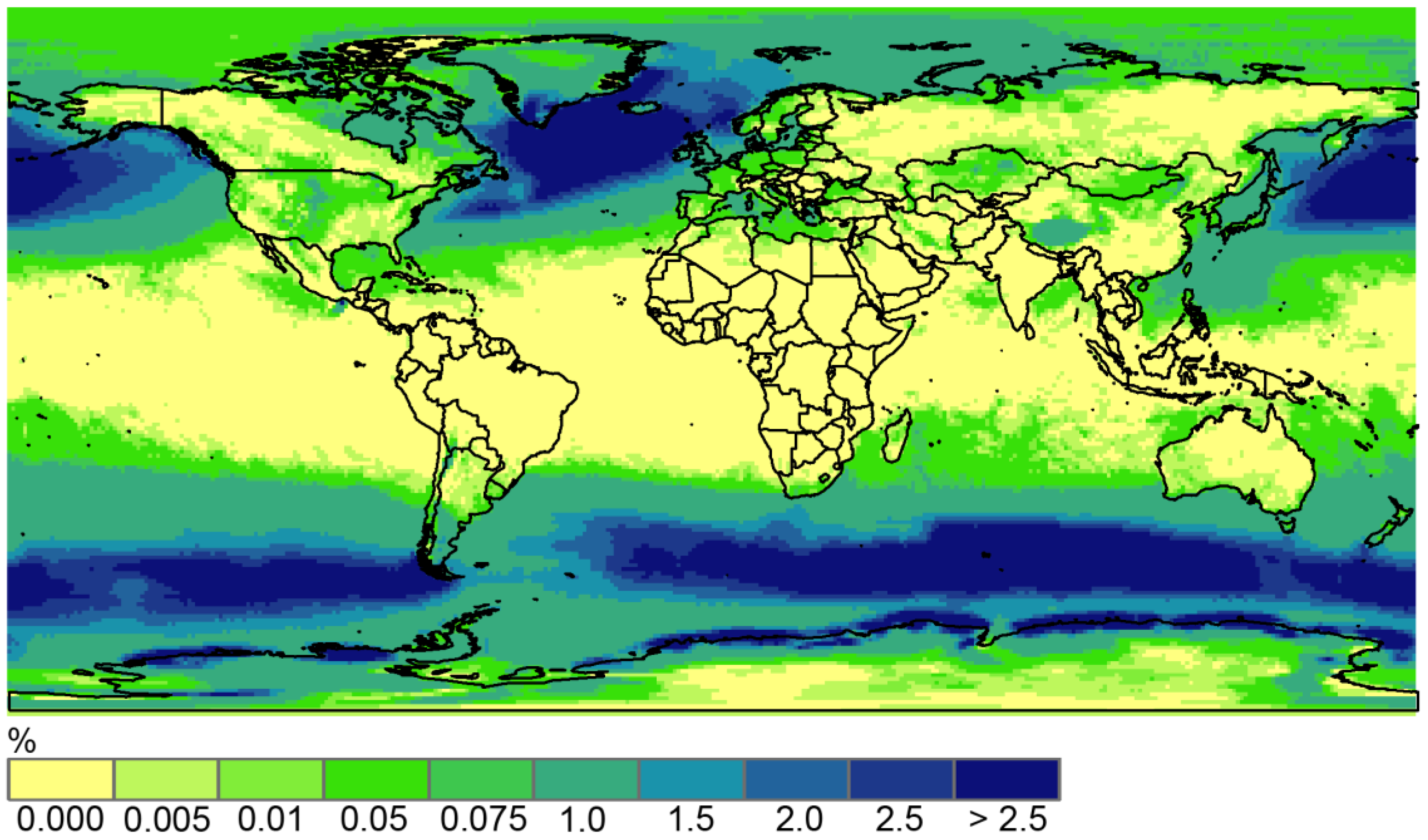
Frequently recurring periods of GS exceeding cut-out speed can lead to energy yield loss. Such conditions occur over the ocean areas of the mid-latitudes where SOC often exceeds 2.5% (Figure 2). Onshore areas are clearly less affected by SOC > 2.5%. They are limited to some regions near the coast of Chile, western Ireland and Great Britain, Canada, Alaska, Greenland, and Iceland. On the Changtang plateau in China, SOC exceeds 0.25% in vast areas. In large parts of mid-latitude countries like Canada, USA, Argentina, Japan, and the western European countries, SOC values exceed 0.01%. As can be clearly seen, very low SOC values dominate in the low latitudes and near the equator. In northern parts of South America, Africa, India, and Southeast Asia, almost no periods where GS > 25 m s−1 occur. Exceptions are where tropical cyclones are frequent such as the Gulf of Mexico, near Madagascar, and the Bay of Bengal. Overall, at 27.8% of all grid cells SOC = 0. On the other hand, GS exceeds 25 m s−1 during 2.5% of all periods at 8.1% of all grid cells.
Surface roughness disturbs the laminar air flow. Consequently, air flow over rough surfaces becomes more turbulent and gust factors increase [46]. Therefore, high values can be found where surface roughness is high (Figure 3). In areas where tropical forests dominate, is often > 3.0. Beside tropical forests, large mountain ranges cause high surface roughness, and consequently high values. Such conditions can be found in the Rocky Mountains, the Alps and the Himalaya, where values related to tropical forests are even exceeded ( > 4.0). In Japanese onshore areas, values lie between 2.5 and 3.0. Lowest can be found over ocean areas, Greenland and the Antarctica ( ~ 1.4). Over European land areas, is often ~2.0. In the Midwestern of the United States, the Sahara and Kazakhstan, low values were simulated, indicating that the negative influence of gusts on the technical integrity is small. Overall, at 35.9% of all grid cells is below 1.4. At 84.8% of all grid cells, does not exceed 2.0. Very high values (>3.0) can be found on 2.5% of the earth’s surface.
3.3. Monthly Gust Characteristics
In many regions around the world, GS characteristics vary within a year. Therefore, annual cycles of GS50yr, SOC and are presented for six grid cells in Figure 4. These grid cells represent regions of the six countries with the highest CO2 emissions in 2015 [47], where high values offer a good meteorological wind energy potential and are not restricted due to geographical constraints. Highest GS50yr values for a grid cell related to China (24.02° N, 117.61° E) occur in July and October (29 m s−1) (Figure 4a). SOC values throughout the year are low. Only in July and October GS values above 25.0 m s−1 occur. It is remarkable that highest values (>600 W m−2) were simulated in November and December, when GS50yr does not exceed 24.0 m s−1 and SOC = 0.0%. This example demonstrates that highest and GS can occur independently of each other. In contrast to GS50yr, SOC and , is nearly constant throughout the year. In June, July, and August is 1.6, whereas in all other months = 1.5.
Highest GS50yr values related to a grid cell in the USA (35.91° N, 100.18° W) occur in April (Figure 4b). In the same month, SOC (0.3%) and (343 W m−2) exceed the values related to all other months. Lowest GS50yr (19 m s−1) and (158 W m−2) was simulated in August. The values (1.7–1.8) are slightly higher than at the grid point related to China, indicating a more pronounced gustiness of the airflow. The variations throughout the year are small. This emphasizes that is rather driven by surface characteristics than by large-scale air flow variations throughout the year.
Due to the Indian monsoon, the regime of a grid cell related to India (8.32° N, 77.72° E) is characterized by two maxima (Figure 4c). The highest values of the first maximum occurring in summer were simulated in June (806 W m−2). In winter, when the second maximum happens, reaches values up to 488 W m−2. The GS50yr values are comparatively low (<20 m s−1). The values lie in the range of 1.4–1.6. GS values exceeding 25.0 m s−1 were not simulated in the investigation period, therefore SOC = 0.0% in all months.
In Japan (40.70° N, 141.12° E), values in winter are clearly higher (>800 W m−2) than in summer ( > 150 W m−2) (Figure 4d). The highest GS50yr values occur in February (40 m s−1). In September, GS50yr = 34 m s−1, although is rather low (205 W m−2). This is due to the influence of typhoons, which only last for a short period, so that their influence on is small. From August to April, GS exceeds 25 m s−1 several times (0.1–0.7%). In contrast to results presented for China, the USA and India the values in summer (~1.4) are lower than in winter (~1.6). Thus, it must be noted that the great wind energy potential in winter is accompanied by gusts.
In Russia (61.30° N, 32.26° E), the highest values were simulated in November (408 W m−2) (Figure 4e). The GS50yr maximum (25.0 m s−1) is simulated in the same months. Lowest (100 W m−2) and GS50yr (19 m s−1) occur in July. Cut-out wind speed is not exceeded (SOC = 0.0%). Thus, losses due to shut-downs of wind turbines during storm events are no serious issue in this region. The values lie between 1.4–1.5 throughout the year, indicating an overall low turbulence.
The yearly cycle for a grid cell related to Northwestern Germany (53.58° N, 7.29° E) is characterized by a maximum in January (1070 W m−2) and a minimum in July (326 W m−2) (Figure 4f). The high values are accompanied by extreme GS50yr values (December and January: 36 m s−1). In contrast to all other examples presented so far, SOC values exceed 1.0% from November to February. Northwestern Germany is regularly influenced by windstorms in winter. Although these events ensure great wind energy potential, the windstorm-related gusts must be recognized as being potentially destructive and causing periods where no wind energy can be generated. The values are low throughout the whole year (1.4).
In Figure 5, annual cycles of GS50yr, SOC and are presented for six regions, which offer a good to great wind energy potential (>700 W m−² in one month). The extreme wind climate related to a grid point near the Canadian east coast (53.60° N, 56.34° W) is characterized by very high GS50yr values that exceed 30 m s−1 in all months, except June, July and August (Figure 5a). The highest GS50yr values were simulated in March (41 m s−1). From November to February, ( > 1000 W m−2). However, periods where GS exceeds cut-out speed are frequent, with the highest SOC values occurring from December to February (4.7%, 5.2%, and 3.8%). Only in June, July, and August SOC = 0.0%. The values are 1.4 throughout the whole year.
The annual variation in Argentina (51.86° S, 69.12° W) is relatively small. The values lie between 610 W m−2 in May and 895 W m−2 in November (Figure 5b). Except for July, GS50yr is at least 30 m s−1 in all months, but does not exceed 35 m s−1. Periods where GS > 25.0 m s−1 occur on a regular base, ranging from 0.4% in July to 1.4 in November and February. Thus, losses due to high GS values must be considered. The gustiness of the airflow is small, therefore lies between 1.4 in November and December and 1.5 in all other months.
The annual GS characteristics for a grid point related to Great Britain (57.61° N, 2.07° W) are similar to those presented for Canada (Figure 5c). The percentage share of GS > 25.0 m s−1 exceeds 1.0% between November and March. In January GS50yr reaches 41 m s−1. The lowest GS50yr was simulated in June (24 m s−1). The values related to the grid cell are higher than 900 W m−2 between October and March. From May to August, the wind energy potential is smaller ( < 400 W m−2). The variable that has the lowest variability throughout the year is . Except for December (1.5), it is 1.4 in all months.
The GS properties related to a grid point of the Western Sahara (25.64° N, 14.55° W) greatly differ from the previously presented results (Figure 5d). In the Western Sahara, northeasterly trade winds dominate, whereas the wind climate in Canada, Argentina, and Great Britain is mainly influenced by the west wind drift. GS50yr does not exceed 25 m s−1, consequently SOC is 0 in all months. From March to October GS50yr is below 20 m s−1. The highest GS50yr value (23 m s−1) occurs in February. The surface roughness in the Western Sahara is low, thus is only 1.4 in all months. The maximum of the trade winds occurs in July, therefore ( = 941 W m−2). The lowest value was simulated in November (310 W m−2).
The Indian summer monsoon is a special case of trade winds, which induces southwesterly airflow at the Horn of Africa. Thus, in Somalia (9.37° N, 50.60° E) values in June (2294 W m−2), July (2873 W m−2) and August (2516 W m−2) are exceptionally high (Figure 5e). Nevertheless, GS50yr does not exceed 25 m s−1 in these months. These values indicate that air flow is constant, but not gusty. Consequently, values are very low, especially in August (1.3). Such conditions are very favorable for wind energy utilization. The northeasterly winter monsoon leads to a secondary maximum from November to February, where values are between 329 W m−2 and 683 W m−2. The corresponding GS50yr values are below 20 m s−1. In April lowest values are simulated (96 W m−2).
In Australia (37.71° S, 140.42° E), the highest GS50yr values (30 m s−1) occur in August and September (Figure 5f). The monthly GS50yr variability is small, since the lowest GS50yr value in February is 25 m s−1. The SOC values between March and October are in the range between 0.1% and 0.4%. In all other months GS50yr values do not exceed 25.0 m s−1. Similar to the annual GS50yr cycle the maximum values were simulated in August (813 W m−2). The values are low throughout the whole year (1.4).
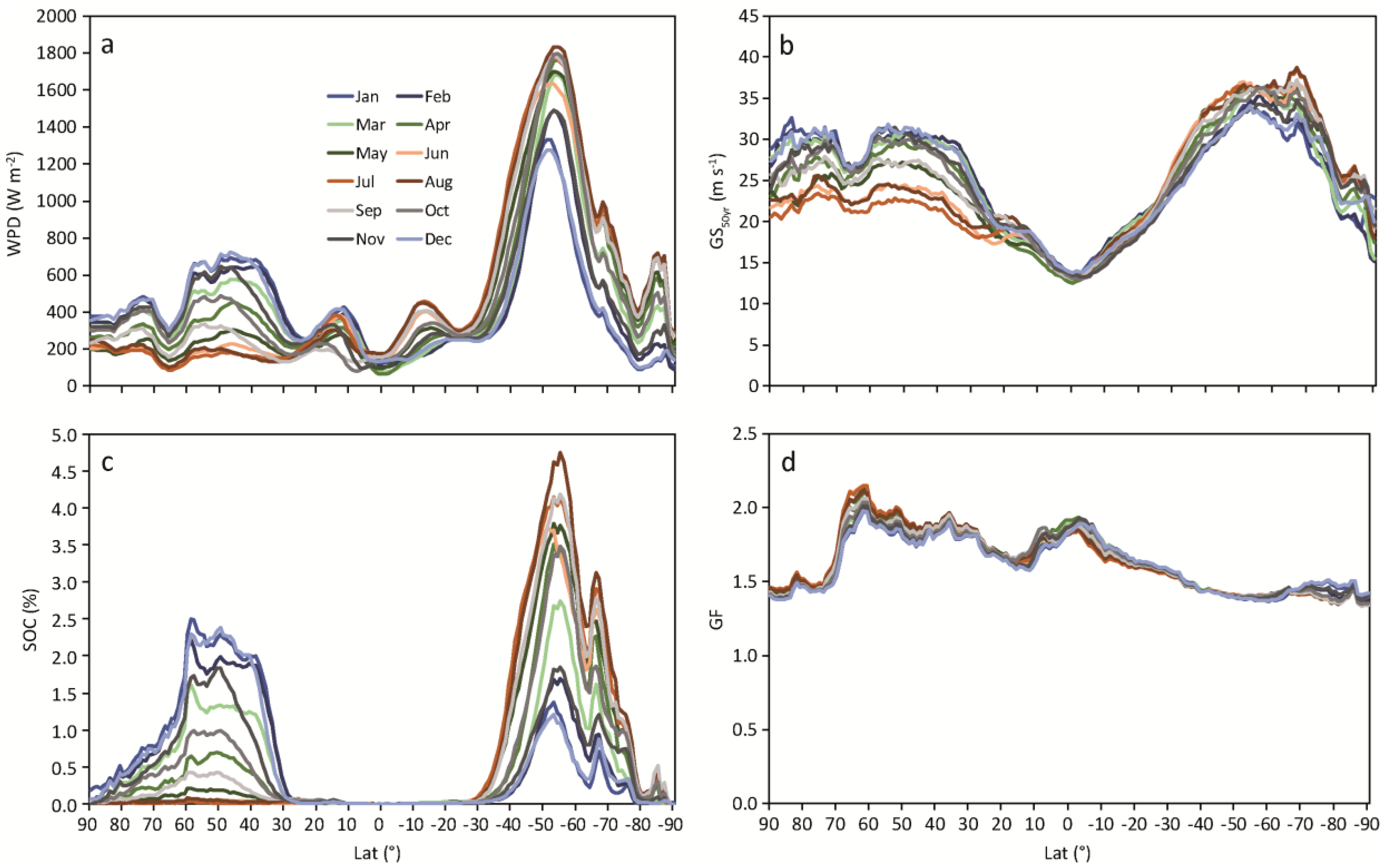
The results that were presented in the previous section showed that the latitude has a great influence on GC. In order to highlight its impact, GS50yr, SOC, and were averaged over all longitudes separately for all months. For better comparability was also averaged over all longitudes and is presented in Figure 6a. It reveals that meteorological wind energy potential is highest between 40° S and 70° S, where peaks at 54° S in August (1834 W m−2). values in this area are highest in all months, but most clearly exceed values of all other latitudes from June to August. The corresponding latitudes of the northern hemisphere are characterized by clearly lower values and a pronounced annual cycle. This is due to the rough surfaces of the continents, whereas the southern hemisphere is predominantly covered by oceans. The lowest can be found at the equator in April (64 W m−2). Local maxima occur between 10° N and 20° N in the winter months and 10° S and 20° S in the summer months.
The distribution of GS50yr values shows some differences from (Figure 6b). With increasing proximity to the equator, GS50yr values decrease virtually linear to 12 m s−1 in April. This is due to the fact that trade winds are constant rather than gusty. The maximum GS50yr value occurs at 67° S in July and August. This is near the Antarctic shore, where the transition zone between water and ice induces high GS values. The mid-latitudes of the northern hemisphere show a profound annual cycle with minimum GS50yr values in July and maximum GS50yr values in December and January.
The monthly SOC values are presented in Figure 6c. Virtually no GS values exceed 25.0 m s−1 between 30° N and 30° S. The maximum SOC value in January is at 58° N (2.49%), whereas the maximum SOC value in August is at 55° S (4.74%). These results indicate that the extratropical cyclones are the main reasons for GS values exceeding cut-out speed, and thus induce periods where no wind energy can be produced.
Since is mainly influenced by surface roughness, their variability is determined by the distributions of land and ocean surfaces (Figure 6d). Highest values (2.2) were simulated at 61° N in June. At this latitude, the land surfaces of Russia and Canada cover large parts of the earth surface. The monthly variability of is due to the fact that increases with decreasing x, which occur at the mid-latitudes in summer months. The minimum value occurs at 82° S from March to October (1.3). This is due to the low surface roughness of the Antarctic ice sheet.
3.4. Wind Turbine Gust Index
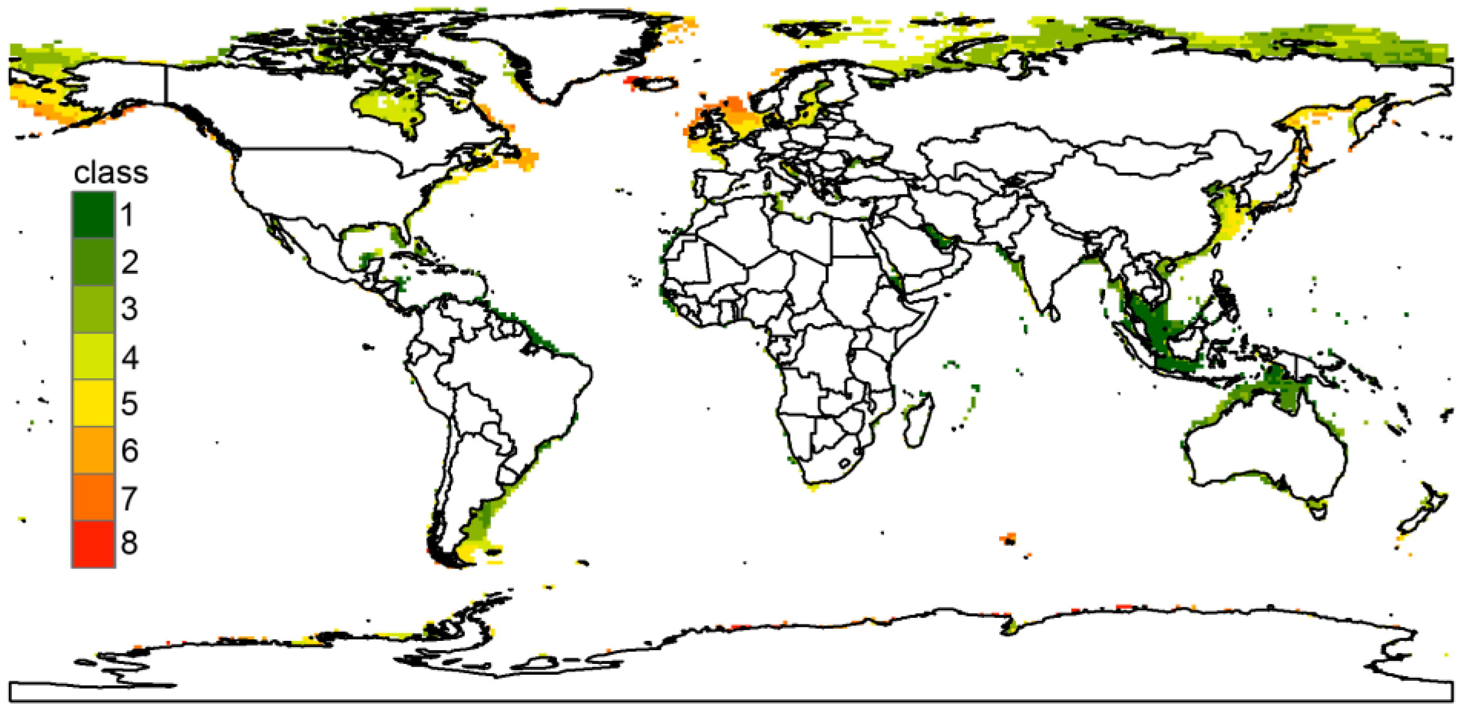
The variables GS50yr, SOC and were integrated into WTGI to yield a relative assessment of the influence of gusts on wind turbines and power generation. The global distribution of onshore WTGI is presented for all non-geographically restricted areas without considering (Figure 7a) and where > 50 W m−2 (Figure 7b). The largest continuous areas that are most seriously negatively affected by gusts (WTGI = 8) and where exceeds 50 W m−2 can be found in the Northeastern United States, in Southeast Canada, Newfoundland, the southern tip of South America, and Northwestern Europe. The west coast of North America, Iceland, South Africa, northern parts of Madagascar, west coast of Scandinavia, Tasmania, New Zealand, South Korea, Japan, the Midwestern United States, and parts of Northeast China are also characterized by high WTGI values. Lowest WTGI values in areas, where > 50 W m−2, mainly occur in eastern Brazil, in the Sahara, southern parts of Somalia, and southeastern parts of the Arabian Peninsula. These results indicate that areas where trade winds dominate are less influenced by negative gust effects than areas in the mid-latitudes.
exceeds 50 W m−2 in almost all offshore areas (Figure 8). Highest WTGI offshore values can be found near Alaska and Iceland. In the North Sea region, the Sea of Okhotsk, and the Canadian east coast, high WTGI values indicate a strong influence of GS. Lowest WTGI values occur along the northwestern coast of South America, the Red Sea, the Persian Gulf, Southeast Asia, and the Arafura Sea.
4. Conclusions
The influence of gust characteristics on wind energy production was assessed at the global scale. It was found that in the mid-latitudes, where the west wind drift dominates, wind turbines are exposed to gust speeds that frequently exceed cut-out speed and lead to shut-downs of wind turbines. In regions where the trade winds dominate, the frequency of gust speeds that disturb wind energy production is much lower. In areas with rough surfaces (e.g., forests or large mountain ranges) the high level of gustiness may also negatively influence the technical integrity of wind turbines. The effects of gusts on wind turbine operations were classified by integrating gust characteristics into the wind turbine gust index WTGI.
The presented assessment of the influence of gust characteristics on wind energy production will be helpful for future large-scale and globally coordinated planning of wind turbine installation. In areas where surface properties influence gust characteristics at the local scale, it is suggested to develop the methodology further to a high spatial resolution assessment. From a previous study an approach exists that allows for mapping gust speed distributions on a high spatial resolution (50 m × 50 m) scale in small study areas [13]. In that study, Wakeby parameters were modeled by an LSBoost approach using sector and distance-limited predictors of surface roughness and terrain-related variables (curvature, elevation, topographic exposure) as well as on ERA-Interim reanalysis wind speed data available at the 850 hPa pressure level. Combining the methodologies of both studies enables the development of gust characteristic maps on a high spatial resolution scale in small study areas. One important requirement to adopt the methodology to small study areas is that long-term gust speed time series exist.
Author Contributions
Christopher Jung conceived and designed the study; Alexander Buchholz, Christopher Jung and Jessica Laible analyzed the data; Dirk Schindler provided guidance; Christopher Jung wrote the paper; Dirk Schindler co-wrote the paper.
Conflicts of Interest
The authors declare no conflict of interest.
Nomenclature
| Acronyms | |
| cdf | cumulative distribution function |
| ecdf | empirical cumulative distribution function |
| epdf | empirical probability density function |
| G | two-parameter Gamma distribution |
| GEV | three-parameter Generalized Extreme Value distribution |
| GL | three-parameter Generalized Logistic distribution |
| GN | three-parameter Generalized Normal distribution |
| GoF | goodness-of-fit |
| GP | three-parameter Generalized Pareto distribution |
| Gu | two-parameter Gumbel distribution |
| K | four-parameter Kappa distribution |
| L | two-parameter Lognormal distribution |
| L3 | three-parameter Lognormal distribution |
| LM | L-moment method |
| M | Moment method |
| ML | Maximum Likelihood estimation |
| P3 | three-parameter Pearson 3 distribution |
| PEM | parameter estimation method |
| S | abbreviation |
| Wak | five-parameter Wakeby distribution |
| Wei | two-parameter Weibull distribution |
| Symbols | |
| estimated cumulative distribution function | |
| median gust factor | |
| mean wind power density | |
| AD | Anderson–Darling statistic |
| APR | atmospheric pressure |
| F | cumulative distribution function |
| F−1 | quantile function |
| GC | gust characteristic |
| GC′ | normalized gust characteristic |
| GF | gust factor |
| GS | gust speed |
| KS | Kolmogorov–Smirnov statistic |
| Lat | latitude |
| Lon | longitude |
| n | sample size |
| NP | number of parameters |
| R | atmospheric gas constant |
| RP | return period |
| SOC | percentage number of exceedances of cut-out speed |
| TA | air temperature |
| T | return period |
| u | zonal wind vector component |
| v | meridional wind vector component |
| WPD | wind power density |
| WTGI | wind turbine gust index |
| x | wind speed |
| α | first scale parameter |
| β | first shape parameter |
| γ | second scale parameter |
| δ | second shape parameter |
| ε | location parameters |
| air density | |
| Subscripts | |
| 100yr | 100-year return period |
| 30yr | 30-year return period |
| 50yr | 50-year return period |
| max | maximum |
| min | minimum |
| i | ith value of data sample |
| WAK | Wakeby distribution |
References
- Payne, J.E. A survey of the electricity consumption-growth literature. Appl. Energy 2010, 87, 723–731. [Google Scholar] [CrossRef]
- Panteli, M.; Mancarella, P. Influence of extreme weather and climate change on the resilience of power systems: Impacts and possible mitigation strategies. Electr. Power Syst. Res. 2015, 127, 259–270. [Google Scholar] [CrossRef]
- Campbell, R.J. Weather-Related Power Outages and Electric System Resiliency; Congressional Research Service: Washington, DC, USA, 2012.
- Cadini, F.; Agliardi, G.L.; Zio, E. A modeling and simulation framework for the reliability/availability assessment of a power transmission grid subject to cascading failures under extreme weather conditions. Appl. Energy 2017, 185, 267–279. [Google Scholar] [CrossRef]
- He, W.; Ge, S.S. Vibration control of a nonuniform wind turbine tower via disturbance observer. IEEE ASME Trans. Mechatron. 2015, 20, 237–244. [Google Scholar] [CrossRef]
- Durst, C.S. Wind speeds over short periods of time. Meteorol. Mag. 1960, 89, 181–186. [Google Scholar]
- Jung, C.; Schindler, D.; Albrecht, A.; Buchholz, A. The role of highly-resolved gust speed in simulations of storm damage in forests at the landscape scale: A case study from southwest Germany. Atmosphere 2016, 7, 7. [Google Scholar] [CrossRef]
- Wang, J.; Qin, S.; Jin, S.; Wu, J. Estimation methods review and analysis of offshore extreme wind speeds and wind energy resources. Renew. Sustain. Energy Rev. 2015, 42, 26–42. [Google Scholar] [CrossRef]
- Quaschning, V. Regenerative Energiesysteme. Technologie—Berechnung—Simulation, 9th ed.; Carl Hanser Verlag GmbH & Co.: München, Germany, 2011; ISBN 978-3-446-44267-2. [Google Scholar]
- Morgan, E.C.; Lackner, M.; Vogel, R.M.; Baise, L.G. Probability distributions for offshore wind speeds. Energy Convers. Manag. 2011, 52, 15–26. [Google Scholar] [CrossRef]
- Lydia, M.; Kumar, S.S.; Selvakumar, A.I.; Prem Kumar, G.E. A comprehensive review on wind turbine power curve modeling techniques. Renew. Sustain. Energy Rev. 2014, 30, 452–460. [Google Scholar] [CrossRef]
- Manwell, J.F.; McGowan, J.G.; Rogers, A.L. Wind Energy Explained: Theory, Design and Application, 2nd ed.; John Wiley & Sons: Chichester, UK, 2009; ISBN 978-0470015001. [Google Scholar]
- Jung, C.; Schindler, D. Modelling monthly near-surface maximum daily gust speed distributions in Southwest Germany. Int. J. Climatol. 2016, 36, 4058–4070. [Google Scholar] [CrossRef]
- Haanpää, S.; Lehtonen, S.; Peltonen, L.; Talockaite, E. Impacts of Winter Storm Gudrun of 7th–9th January 2005 and Measures Taken in Baltic Sea Region. Available online: http://www.astra-project.org/06_winterstorm_study.html (accessed on 27 August 2017).
- Lee, B.-H.; Ahn, D.-J.; Kim, H.-G.; Ha, Y.-C. An estimation of the extreme wind speed using the Korea wind map. Renew. Energy 2012, 42, 4–10. [Google Scholar] [CrossRef]
- Chang, P.-C.; Yang, R.-Y.; Lai, C.-M. Potential of Offshore Wind Energy and Extreme Wind Speed Forecasting on the West Coast of Taiwan. Energies 2015, 8, 1685–1700. [Google Scholar] [CrossRef]
- Kang, D.; Ko, K.; Huh, J. Determination of extreme wind values using the Gumbel distribution. Energy 2015, 86, 51–58. [Google Scholar] [CrossRef]
- Pes, M.P.; Pereira, E.B.; Marengo, J.A.; Martins, F.R.; Heinemann, D.; Schmidt, M. Climate trends on the extreme winds in Brazil. Renew. Energy 2017, 109, 110–120. [Google Scholar] [CrossRef]
- Gong, K.; Ding, J.; Chen, X. Estimation of long-term extreme response of operational and parked wind turbines: Validation and some new insights. Eng. Struct. 2014, 81, 135–147. [Google Scholar] [CrossRef]
- Chiodo, E.; De Falco, P. Inverse Burr distribution for extreme wind speed prediction: Genesis, identification and estimation. Electr. Power Syst. Res. 2016, 141, 549–561. [Google Scholar] [CrossRef]
- Dee, D.P.; Uppala, S.M.; Simmons, A.J.; Berrisford, P.; Poli, P.; Kobayashi, S.; Andrae, U.; Balmaseda, M.A.; Balsamo, G.; Bauer, P.; et al. The ERA-Interim reanalysis: Configuration and performance of the data assimilation system. Q. J. R. Meteorol. Soc. 2011, 137, 553–597. [Google Scholar] [CrossRef]
- WMO Guide to Meteorological Instruments and Methods of Observations. Available online: https://library.wmo.int/opac/doc_num.php?explnum_id=3177 (accessed on 27 August 2017).
- Hellman, G. Über die Bewegung der Luft in den untersten Schichten der Atmosphäre. Meteorol. Z. 1915, 32, 1–16. (In German) [Google Scholar]
- Deacon, E.L. Gust variation with height up to 150 m. Q. J. R. Meteorol. Soc. 1955, 81, 562–573. [Google Scholar] [CrossRef]
- Grau, L.; Jung, C.; Schindler, D. On the annual cycle of meteorological and geographical potential of wind energy: A case study from Southwest Germany. Sustainability 2017, 9, 1169. [Google Scholar]
- Kim, J.-Y.; Kim, H.-G.; Kang, Y.-H. Offshore wind speed forecasting: The correlation between satellite-observed monthly sea surface temperature and wind speed over the seas around the Korean peninsula. Energies 2017, 10, 994. [Google Scholar]
- Cehak, K. Der Jahresgang der monatlichen höchsten Windgeschwindigkeiten in der Darstellung durch Fisher-Tippett III-Verteilungen. Arch. Meteorol. Geophys. Bioklimatol. 1971, 19, 165–182. (In German) [Google Scholar] [CrossRef]
- Friederichs, P.; Göber, M.; Bentzien, S.; Lenz, A.; Krampitz, R. A probabilistic analysis of wind gusts using extreme value statistics. Meteorol. Z. 2009, 18, 615–629. [Google Scholar] [CrossRef] [PubMed]
- Jung, C.; Schindler, D. Global comparison of the goodness-of-fit of wind speed distributions. Energy Convers. Manag. 2017, 133, 216–234. [Google Scholar] [CrossRef]
- Massey, F.J. The Kolmogorov-Smirnov test for goodness of fit. J. Am. Stat. Assoc. 1951, 46, 68–78. [Google Scholar] [CrossRef]
- Anderson, T.W.; Darling, D.A. A test of goodness of fit. J. Am. Stat. Assoc. 1954, 49, 765–769. [Google Scholar] [CrossRef]
- Jung, C.; Schindler, D.; Laible, J.; Buchholz, A. Introducing a system of wind speed distributions for modeling properties of wind speed regimes around the world. Energy Convers. Manag. 2017, 144, 181–192. [Google Scholar] [CrossRef]
- Houghton, J.C. Birth of a parent: The Wakeby distribution for modeling flood flows. Water Resour. Res. 1978, 14, 1105–1109. [Google Scholar] [CrossRef]
- Jung, C. High spatial resolution simulation of annual wind energy yield using near-surface wind speed time series. Energies 2016, 9, 344. [Google Scholar] [CrossRef]
- Rahman, A.; Zaman, M.A.; Haddad, K.; El Adlouni, S.; Zhang, C. Applicability of Wakeby distribution in flood frequency analysis: a case study for eastern Australia. Hydrol. Process. 2015, 29, 602–614. [Google Scholar] [CrossRef]
- Hosking, J.; Wallis, J. Regional Frequency Analysis: An Approach Based on L-Moments; Cambridge University Press: Cambridge, UK, 1997. [Google Scholar]
- Schindler, D.; Jung, C.; Buchholz, A. Using highly resolved maximum gust speed as predictor for forest storm damage caused by the high-impact winter storm Lothar in Southwest Germany. Atmos. Sci. Lett. 2016, 17, 462–469. [Google Scholar] [CrossRef]
- Jung, C.; Schindler, D. Development of a statistical bivariate wind speed-wind shear model (WSWS) to quantify the height-dependent wind resource. Energy Convers. Manag. 2017, 149, 303–317. [Google Scholar] [CrossRef]
- Loveland, T.R.; Reed, B.C.; Brown, J.F.; Ohlen, D.O.; Zhu, Z.; Yang, L.; Merchant, J.W. Development of a global land cover characteristics database and IGBP DISCover from 1 km AVHRR data. Int. J. Remote Sens. 2000, 21, 1303–1330. [Google Scholar] [CrossRef]
- The World Database on Protected Areas (WDPA). Available online: https://www.iucn.org/theme/protected-areas/our-work/world-database-protected-areas (accessed on 3 August 2017).
- Danielson, J.J.; Gesch, D.B. Global Multi-Resolution Terrain Elevation Data 2010 (GMTED2010); Open-File Report 2011-1073; U.S. Geological Survey: Reston, VA, USA, 2011.
- Mentis, D.; Hermann, S.; Howells, M.; Welsch, M.; Siyal, S.H. Assessing the technical wind energy potential in Africa a GIS-based approach. Renew. Energy 2015, 83, 110–125. [Google Scholar] [CrossRef]
- Gruber, S. Derivation and analysis of a high-resolution estimate of global permafrost zonation. Cryosphere 2012, 6, 221–233. [Google Scholar] [CrossRef] [Green Version]
- Global Permafrost Zonation Index Map. Available online: http://www.geo.uzh.ch/microsite/cryodata/pf_global/ (accessed on 3 August 2017).
- Lu, X.; McElroy, M.B.; Kiviluoma, J. Global potential for wind-generated electricity. Proc. Natl. Acad. Sci. USA 2009, 106, 10933–10938. [Google Scholar] [CrossRef] [PubMed] [Green Version]
- Wieringa, J. Roughness-dependent geographical interpolation of surface wind speed averages. Q. J. R. Met. Soc. 1986, 112, 867–889. [Google Scholar] [CrossRef]
- Global Carbon Atlas. Available online: http://www.globalcarbonatlas.org/en/CO2-emissions (accessed on 3 August 2017).
Figure 1.
Gust speed (GS) values for a return period of (a) 30 years (GS30yr); (b) 50 years (GS50yr); and (c) 100 years (GS100yr).
Figure 1.
Gust speed (GS) values for a return period of (a) 30 years (GS30yr); (b) 50 years (GS50yr); and (c) 100 years (GS100yr).

Figure 2.
Share of three-hour periods when gust speed (GS) exceeds 25.0 m s−1 (SOC) in the investigation period.
Figure 2.
Share of three-hour periods when gust speed (GS) exceeds 25.0 m s−1 (SOC) in the investigation period.

Figure 3.
Median gust factor () in the investigation period.
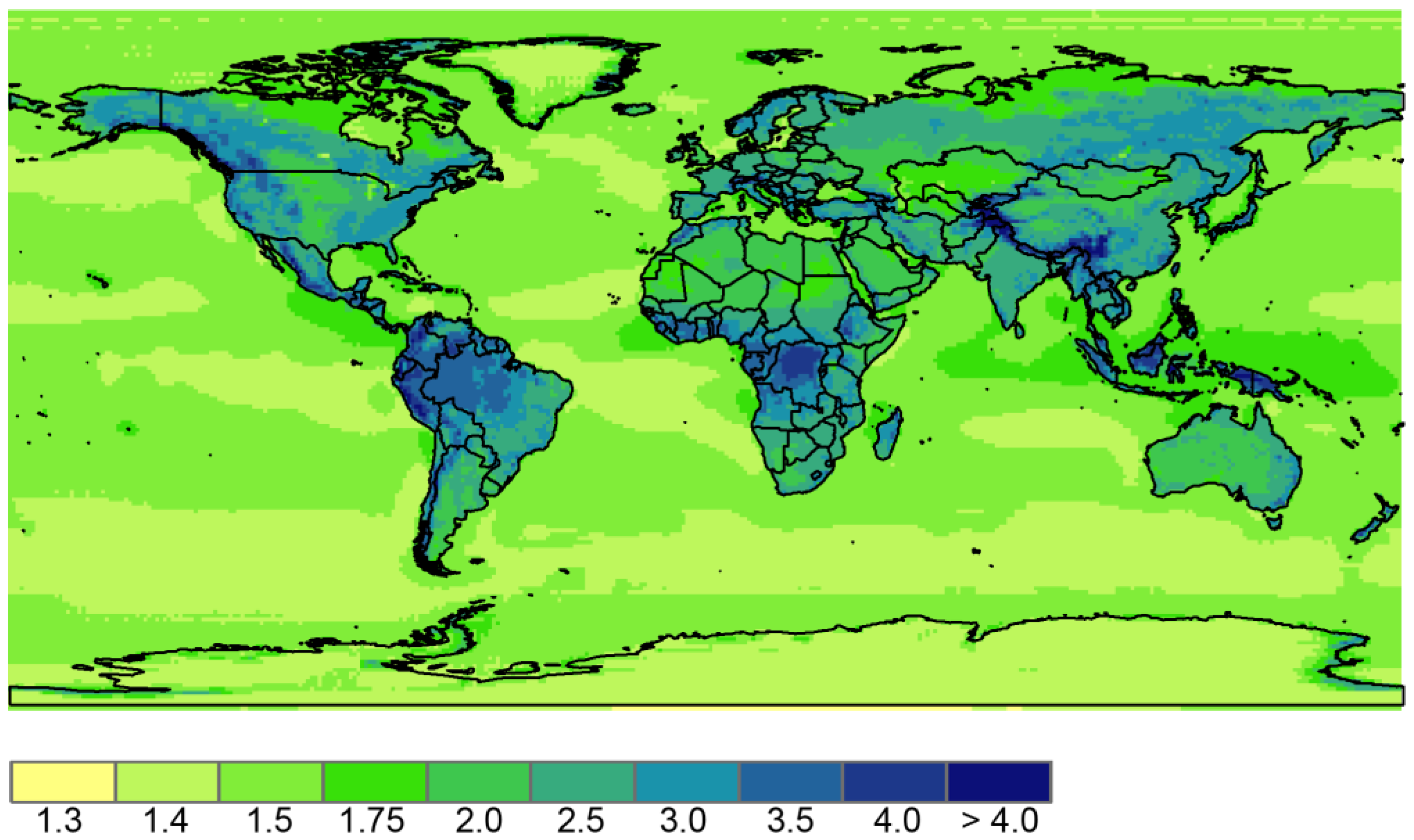
Figure 4.
Annual cycle of monthly gust speed (GS) values for a return period of 50 years (GS50yr), share of three-hour periods when gust speed GS exceeds 25.0 m s−1 (SOC), median gust factor (), and mean wind power density (). Each variable is presented for grid points related to the six countries with highest CO2 emissions in 2015: (a) China; (b) USA; (c) India; (d) Russia; (e) Japan; and (f) Germany.
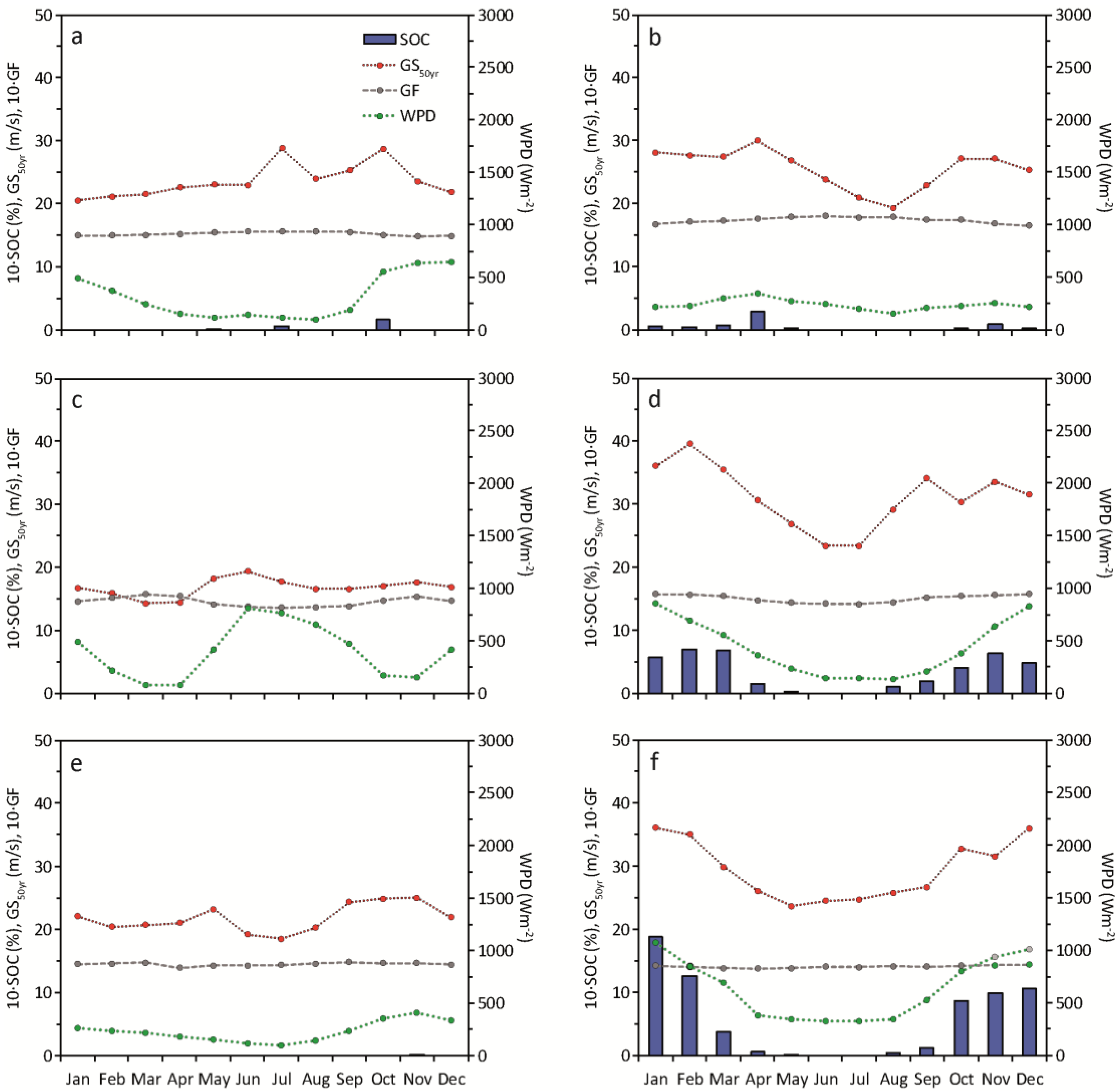
Figure 5.
Annual cycle of monthly gust speed (GS) values for a return period of 50 years (GS50yr), share of three-hour periods when GS exceeds 25.0 m s−1, median gust factor (), and mean wind power density (). Each variable is presented for grid points related to (a) Canada; (b) Argentina; (c) Great Britain; (d) Western Sahara; (e) Somalia; and (f) Australia.
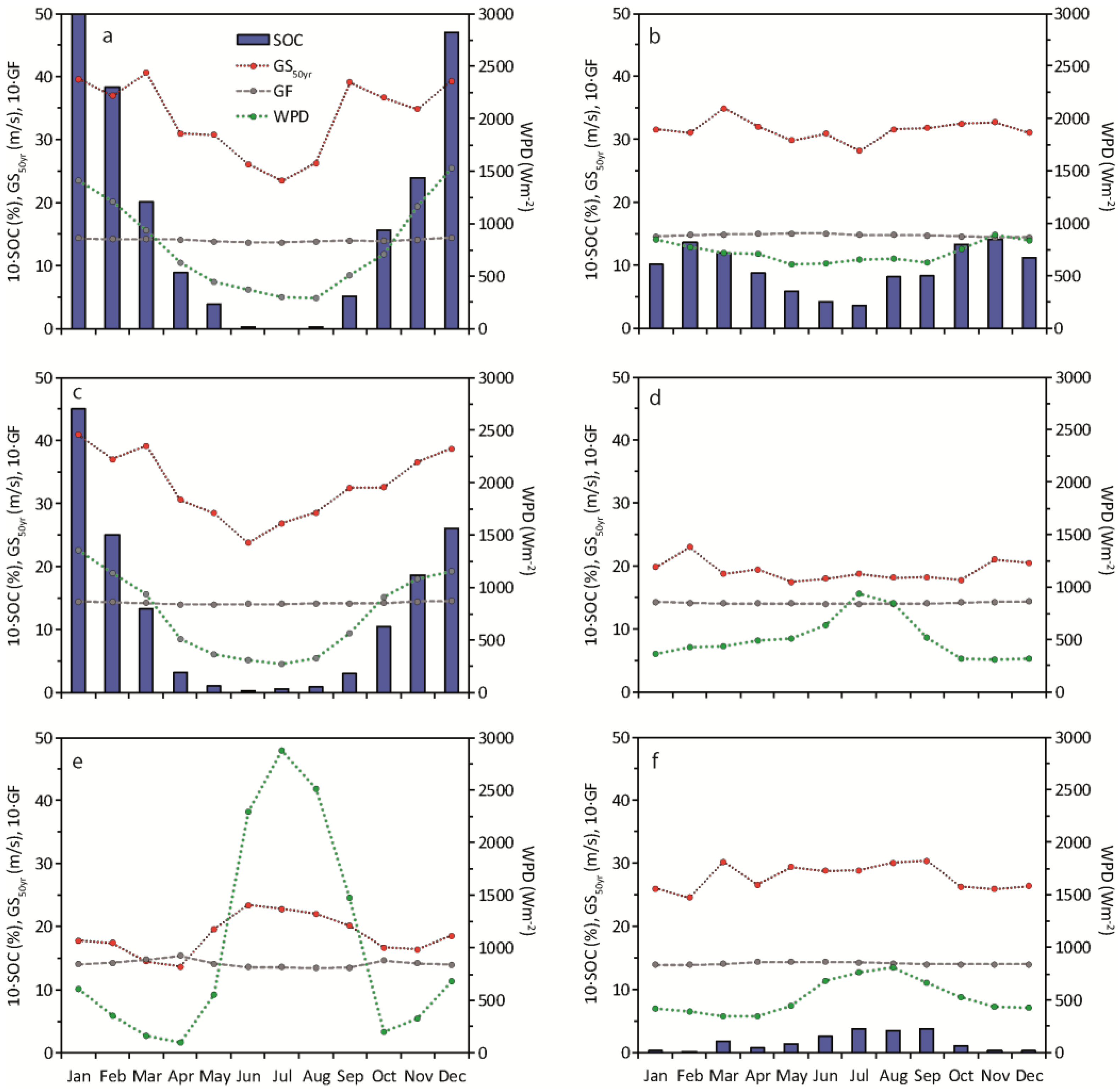
Figure 6.
Monthly (a) mean wind power density (); (b) gust speed (GS) values for a return period of 50 years (GS50yr); (c) share of three-hour periods when GS exceeds 25.0 m s−1 (SOC); and (d) median gust factor () in the investigation period as a function of latitude (Lat). These variables were averaged over all longitudes.

Figure 7.
Global distribution of the onshore wind turbine gust index (WTGI) (a) for all non-geographically restricted areas and (b) for all non-geographically restricted areas where mean wind power density exceeds 50 W m−2.
Figure 7.
Global distribution of the onshore wind turbine gust index (WTGI) (a) for all non-geographically restricted areas and (b) for all non-geographically restricted areas where mean wind power density exceeds 50 W m−2.
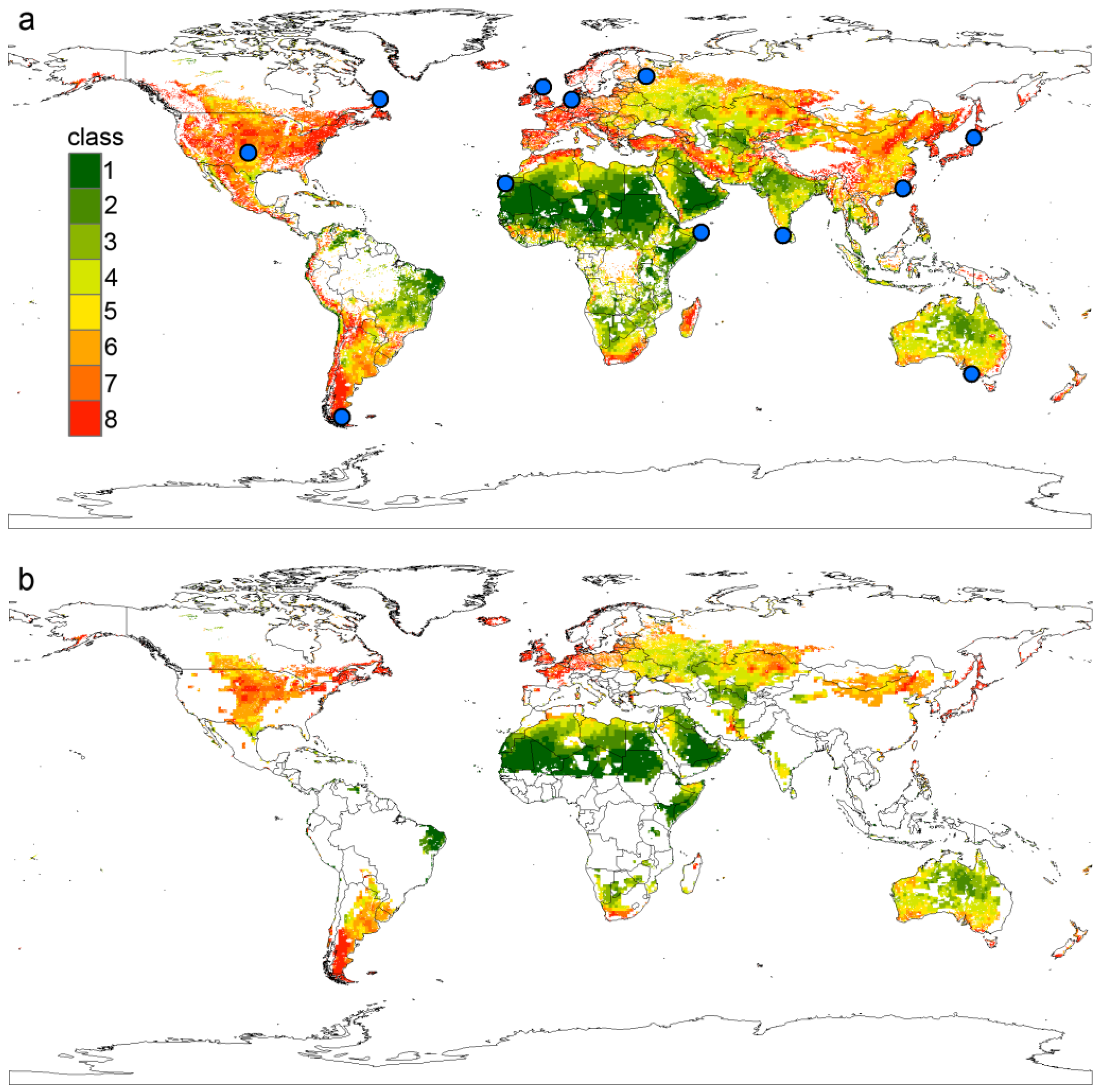
Figure 8.
Global distribution of the offshore wind turbine gust index (WTGI), where sea depth <200 m.
Figure 8.
Global distribution of the offshore wind turbine gust index (WTGI), where sea depth <200 m.


Table 1.
Tested distributions with their abbreviation (S), number of parameters (NP), and parameter estimation methods (PEM).
Table 1.
Tested distributions with their abbreviation (S), number of parameters (NP), and parameter estimation methods (PEM).
| Distribution | S | NP | PEM |
|---|---|---|---|
| Gamma | G | 2 | ML, LM |
| Gumbel | Gu | 2 | ML, LM |
| Lognormal | L | 2 | ML, M |
| Weibull | Wei | 2 | ML, M, LM |
| Gen. Extreme Value | GEV | 3 | ML, LM |
| Generalized Logistic | GL | 3 | LM |
| Gen. Normal | GN | 3 | LM |
| Gen. Pareto | GP | 3 | LM |
| Pearson 3 | P3 | 3 | LM |
| Lognormal | L3 | 3 | LM |
| Kappa | K | 4 | LM |
| Wakeby | Wak | 5 | LM |
Table 2.
Results from goodness-of-fit comparison of the theoretical distributions. The table shows the share of distribution (%) ranked one to three (first number)/best (second number) at all evaluated grid cells according to the comparison of the monthly Kolmogorov–Smirnov (KS) statistic.
Table 2.
Results from goodness-of-fit comparison of the theoretical distributions. The table shows the share of distribution (%) ranked one to three (first number)/best (second number) at all evaluated grid cells according to the comparison of the monthly Kolmogorov–Smirnov (KS) statistic.
| S | Jan | Feb | Mar | Apr | May | Jun | Jul | Aug | Sep | Oct | Nov | Dec |
|---|---|---|---|---|---|---|---|---|---|---|---|---|
| Wak-LM | 66/42 | 66/42 | 66/43 | 67/43 | 67/44 | 66/43 | 67/44 | 67/44 | 66/43 | 66/43 | 67/44 | 67/43 |
| GL-LM | 30/11 | 32/11 | 33/11 | 32/11 | 33/12 | 31/11 | 34/12 | 33/11 | 33/11 | 32/12 | 34/12 | 34/11 |
| K-LM | 29/9 | 28/9 | 28/9 | 28/9 | 27/8 | 29/9 | 27/9 | 27/9 | 27/8 | 28/9 | 27/9 | 28/9 |
| GEV-LM | 24/4 | 24/4 | 26/5 | 25/4 | 24/4 | 25/5 | 24/4 | 25/4 | 24/4 | 25/4 | 26/4 | 25/4 |
| Wei-LM | 22/6 | 21/6 | 21/6 | 22/6 | 21/6 | 22/6 | 21/6 | 21/6 | 22/6 | 21/6 | 21/6 | 21/6 |
| GN-LM | 14/1 | 17/2 | 17/2 | 17/2 | 17/2 | 18/2 | 18/2 | 17/2 | 18/2 | 17/2 | 17/2 | 17/2 |
| GP-LM | 15/5 | 13/4 | 13/4 | 14/4 | 13/4 | 14/4 | 13/4 | 13/4 | 13/4 | 13/4 | 12/4 | 13/4 |
| L3-LM | 15/2 | 13/1 | 13/1 | 12/1 | 13/1 | 13/1 | 13/1 | 13/1 | 13/1 | 13/1 | 12/1 | 12/1 |
| L-ML | 12/2 | 12/2 | 11/2 | 13/2 | 12/2 | 12/2 | 12/2 | 12/2 | 12/2 | 13/2 | 12/2 | 12/2 |
| GEV-ML | 12/3 | 12/3 | 12/3 | 11/3 | 12/3 | 11/3 | 12/3 | 12/3 | 12/3 | 12/3 | 12/3 | 12/3 |
| Gu-ML | 12/4 | 11/3 | 11/3 | 11/3 | 11/3 | 10/3 | 10/3 | 11/3 | 11/3 | 10/3 | 11/3 | 11/3 |
| P3-LM | 10/2 | 11/2 | 11/2 | 10/2 | 10/2 | 10/2 | 10/2 | 10/2 | 11/3 | 10/2 | 10/2 | 10/2 |
| L-M | 10/2 | 10/3 | 9/2 | 10/2 | 10/2 | 10/2 | 10/2 | 10/2 | 10/2 | 10/2 | 10/2 | 10/2 |
| G-LM | 9/2 | 9/2 | 9/2 | 10/2 | 10/2 | 9/2 | 9/2 | 9/2 | 9/2 | 10/2 | 10/2 | 9/2 |
| Gu-LM | 10/2 | 10/3 | 10/2 | 9/2 | 9/2 | 8/2 | 9/2 | 9/2 | 9/2 | 8/2 | 9/2 | 9/2 |
| G-ML | 7/1 | 7/1 | 6/1 | 7/1 | 7/1 | 7/1 | 7/1 | 7/1 | 7/1 | 7/1 | 8/1 | 7/1 |
| Wei-M | 2/0 | 2/0 | 1/0 | 2/0 | 2/0 | 2/0 | 2/0 | 2/0 | 2/0 | 2/1 | 2/0 | 2/0 |
| Wei-ML | 2/0 | 2/0 | 1/0 | 1/0 | 2/0 | 2/0 | 2/0 | 2/0 | 2/0 | 1/0 | 2/0 | 2/0 |
Table 3.
Results from goodness-of-fit comparison of the theoretical distributions. The table shows the share of distribution (%) ranked one to three (first number)/best (second number) at all evaluated grid cells according to the comparison of the monthly Anderson–Darling (AD) statistic.
Table 3.
Results from goodness-of-fit comparison of the theoretical distributions. The table shows the share of distribution (%) ranked one to three (first number)/best (second number) at all evaluated grid cells according to the comparison of the monthly Anderson–Darling (AD) statistic.
| S | Jan | Feb | Mar | Apr | May | Jun | Jul | Aug | Sep | Oct | Nov | Dec |
|---|---|---|---|---|---|---|---|---|---|---|---|---|
| Wak-LM | 61/49 | 62/50 | 62/50 | 62/38 | 64/52 | 62/50 | 62/51 | 62/50 | 62/51 | 63/50 | 62/51 | 63/50 |
| GL-LM | 38/12 | 40/12 | 42/13 | 39/7 | 40/12 | 39/12 | 42/13 | 42/13 | 41/13 | 40/13 | 43/14 | 42/13 |
| GEV-LM | 34/6 | 36/6 | 35/6 | 33/5 | 34/5 | 36/6 | 34/6 | 35/6 | 36/6 | 34/5 | 34/5 | 35/5 |
| K-LM | 32/13 | 31/14 | 31/13 | 55/37 | 30/13 | 32/14 | 30/13 | 30/13 | 29/12 | 31/13 | 30/12 | 31/13 |
| Wei-LM | 32/8 | 30/8 | 29/7 | 31/8 | 31/8 | 33/8 | 31/8 | 30/8 | 30/7 | 31/8 | 30/7 | 30/8 |
| GN-LM | 33/3 | 31/3 | 30/3 | 23/1 | 31/3 | 31/3 | 32/3 | 30/3 | 31/3 | 31/3 | 31/3 | 30/3 |
| L3-LM | 19/2 | 20/2 | 21/2 | 16/1 | 20/2 | 20/2 | 20/2 | 21/2 | 20/2 | 21/2 | 20/2 | 20/2 |
| P3-LM | 18/3 | 17/2 | 16/3 | 15/2 | 16/2 | 16/2 | 16/2 | 16/2 | 16/2 | 17/3 | 15/2 | 16/2 |
| GEV-ML | 10/1 | 10/1 | 11/1 | 7/0 | 9/1 | 9/1 | 9/1 | 10/1 | 10/1 | 9/1 | 10/1 | 11/1 |
| Gu-ML | 5/1 | 4/1 | 5/1 | 4/1 | 4/1 | 4/1 | 4/1 | 5/1 | 4/1 | 4/1 | 4/1 | 5/1 |
| Gu-LM | 4/0 | 4/0 | 5/0 | 4/0 | 4/0 | 4/0 | 4/0 | 5/0 | 5/0 | 4/0 | 4/0 | 4/0 |
| L-ML | 4/0 | 4/0 | 4/0 | 4/0 | 4/0 | 4/0 | 4/0 | 4/0 | 2/0 | 4/0 | 4/0 | 4/0 |
| G-LM | 3/0 | 3/0 | 3/0 | 3/0 | 4/0 | 3/0 | 3/0 | 3/0 | 3/0 | 3/0 | 3/0 | 3/0 |
| G-ML | 2/0 | 2/0 | 2/0 | 2/0 | 4/0 | 2/0 | 2/0 | 2/0 | 2/0 | 2/0 | 2/0 | 2/0 |
| L-M | 2/0 | 2/0 | 2/0 | 1/0 | 4/0 | 2/0 | 2/0 | 2/0 | 2/0 | 2/0 | 2/0 | 2/0 |
| GP-LM | 2/1 | 2/1 | 2/0 | 2/1 | 2/1 | 2/1 | 2/1 | 2/1 | 2/1 | 2/1 | 2/1 | 2/1 |
| Wei-ML | 1/0 | 1/0 | 1/0 | 1/0 | 1/0 | 1/0 | 1/0 | 1/0 | 1/0 | 1/0 | 1/0 | 1/0 |
| Wei-M | 1/0 | 1/0 | 0/0 | 0/0 | 0/0 | 0/0 | 0/0 | 0/0 | 0/0 | 0/0 | 1/0 | 1/0 |
© 2017 by the authors. Licensee MDPI, Basel, Switzerland. This article is an open access article distributed under the terms and conditions of the Creative Commons Attribution (CC BY) license (http://creativecommons.org/licenses/by/4.0/).
Share and Cite
MDPI and ACS Style
Jung, C.; Schindler, D.; Buchholz, A.; Laible, J. Global Gust Climate Evaluation and Its Influence on Wind Turbines. Energies 2017, 10, 1474. https://doi.org/10.3390/en10101474
AMA Style
Jung C, Schindler D, Buchholz A, Laible J. Global Gust Climate Evaluation and Its Influence on Wind Turbines. Energies. 2017; 10(10):1474. https://doi.org/10.3390/en10101474
Chicago/Turabian StyleJung, Christopher, Dirk Schindler, Alexander Buchholz, and Jessica Laible. 2017. "Global Gust Climate Evaluation and Its Influence on Wind Turbines" Energies 10, no. 10: 1474. https://doi.org/10.3390/en10101474
Note that from the first issue of 2016, this journal uses article numbers instead of page numbers. See further details here.